Hall ARCH and GARCH

1. Lecture 8 Stephen G. Hall ARCH and GARCH

2.

REFS
A thorough introduction
‘ARCH Models’ Bollerslev T, Engle R F and Nelson D B
Handbook of Econometrics vol 4. or UCSD Discussion paper
no 93.49. (available on my web site)
A quick survey
Cuthbertson Hall and Taylor

3.

Until the early 80s econometrics had focused almost solely
on modelling the means of series, ie their actual values.
Recently however we have focused increasingly on the
importance of volatility, its determinates and its effects on
mean values.
A key distinction is
unconditional variance.
between
the
conditional
and
the unconditional variance is just the standard measure of
the variance
var(x) =E(x -E(x))2

4.

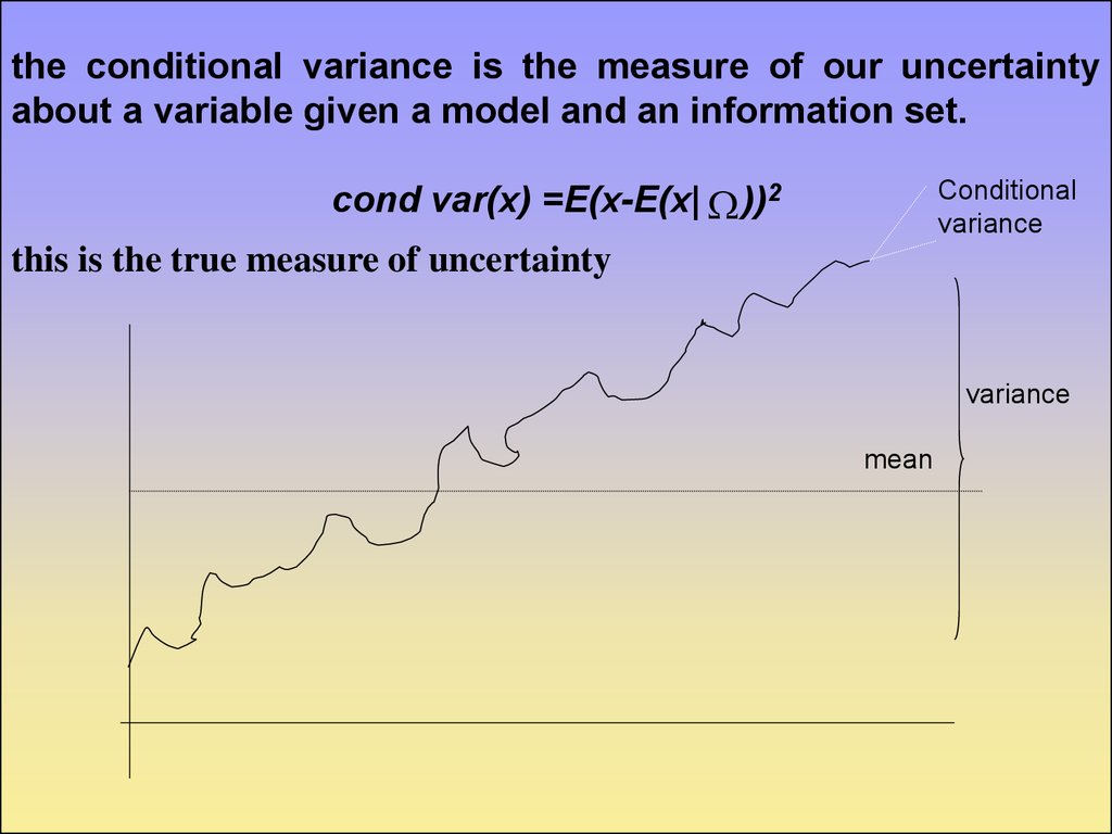
the conditional variance is the measure of our uncertainty
about a variable given a model and an information set.
cond var(x) =E(x-E(x| ))2
Conditional
variance
this is the true measure of uncertainty
variance
mean

5.

Stylised Facts of asset returns
i) Thick tails, they tend to be leptokurtic
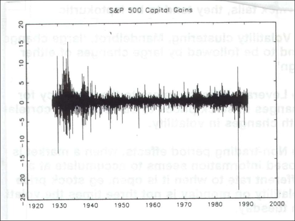
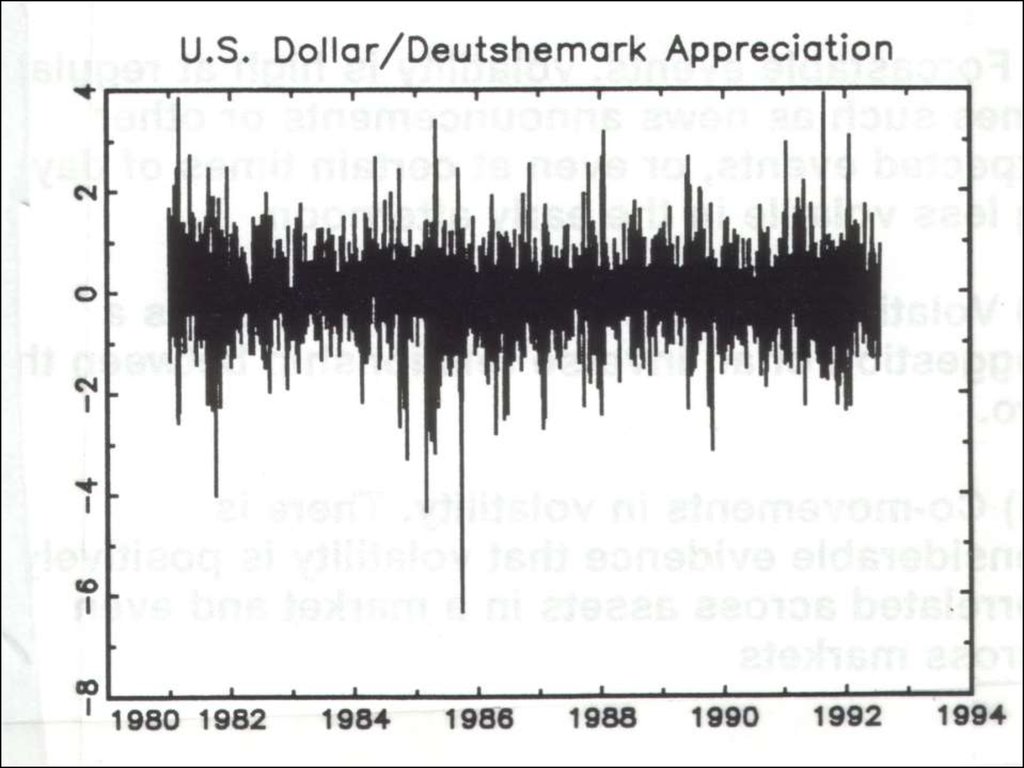
ii)Volatility clustering, Mandelbrot, ‘large changes tend to be
followed by large changes of either sign’
iii)Leverage Effects, refers to the tendency for changes in stock
prices to be negatively correlated with changes in volatility.
iv)Non-trading period effects. when a market is closed information
seems to accumulate at a different rate to when it is open. eg stock
price volatility on Monday is not three times the volatility on
Tuesday.
v) Forcastable events, volatility is high at regular times such
as news announcements or other expected events, or even at
certain times of day, eg less volatile in the early afternoon.

6.

vi)Volatility and serial correlation. There is a suggestion of an
inverse relationship between the two.
vii)
Co-movements in volatility. There is considerable evidence
that volatility is positively correlated across assets in a market and
even across markets

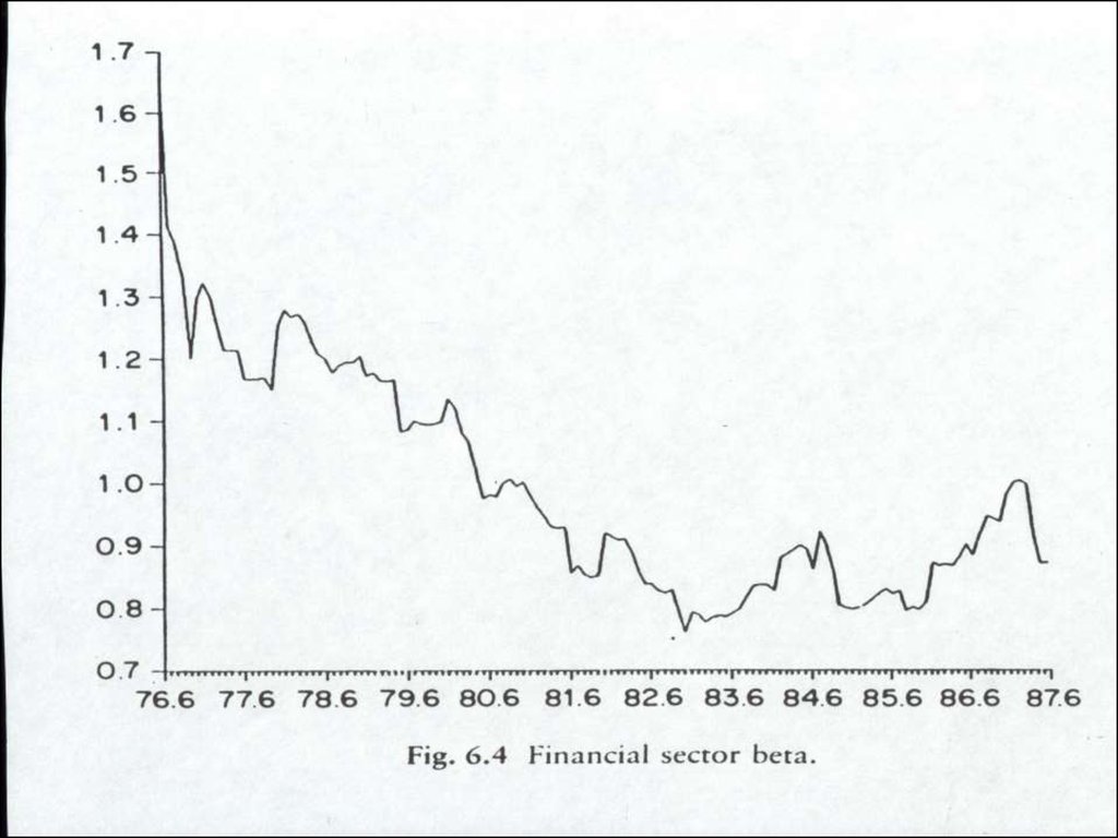
7.

8.

9.

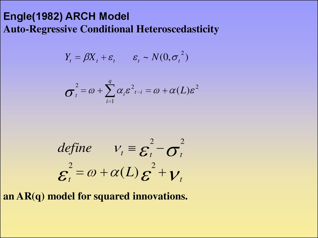
Engle(1982) ARCH Model
Auto-Regressive Conditional Heteroscedasticity
Yt X t t
2
t
t
q
i 2 t i ( L) 2
define
2
t ~ N (0, t 2 )
i 1
t t t
2
2
( L) t
2
an AR(q) model for squared innovations.

10.

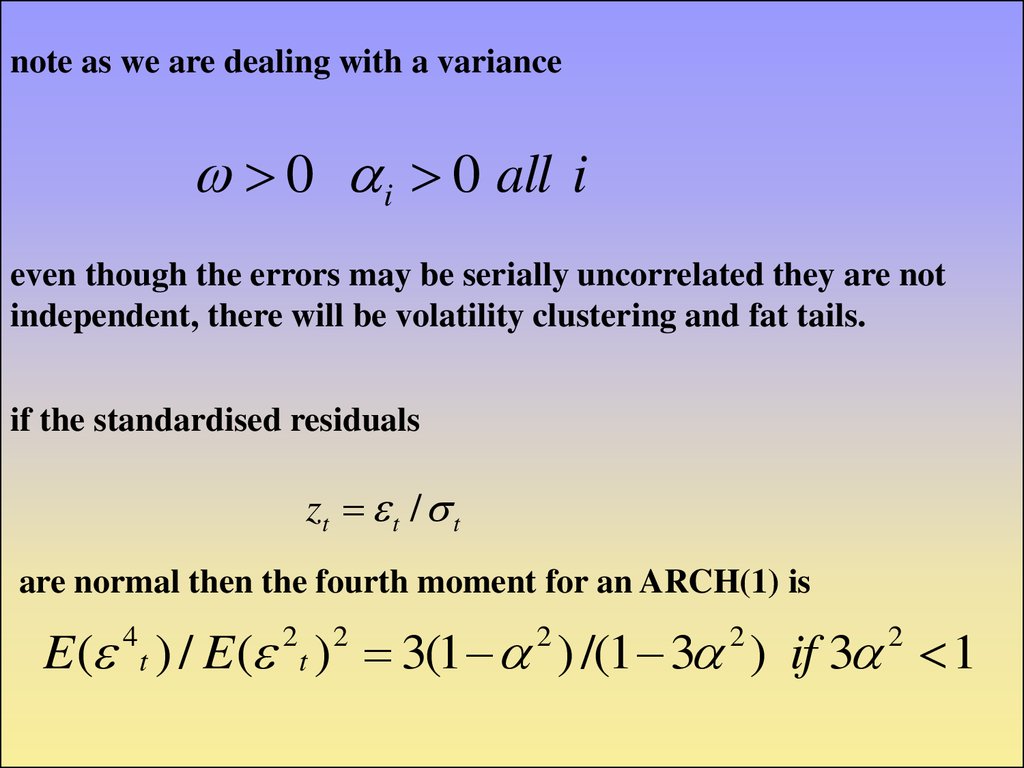
note as we are dealing with a variance
0 i 0 all i
even though the errors may be serially uncorrelated they are not
independent, there will be volatility clustering and fat tails.
if the standardised residuals
zt t / t
are normal then the fourth moment for an ARCH(1) is
E ( t ) / E ( t ) 3(1 ) /(1 3 ) if 3 1
4
2
2
2
2
2

11.

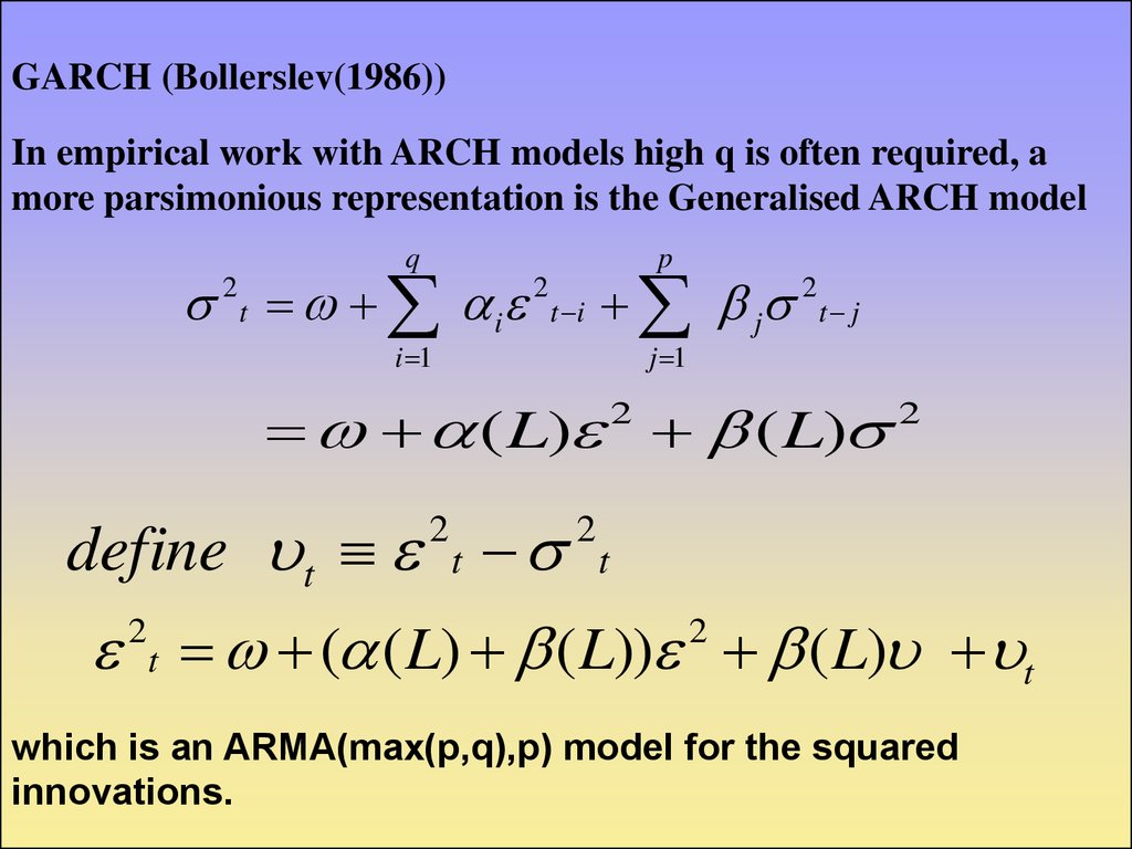
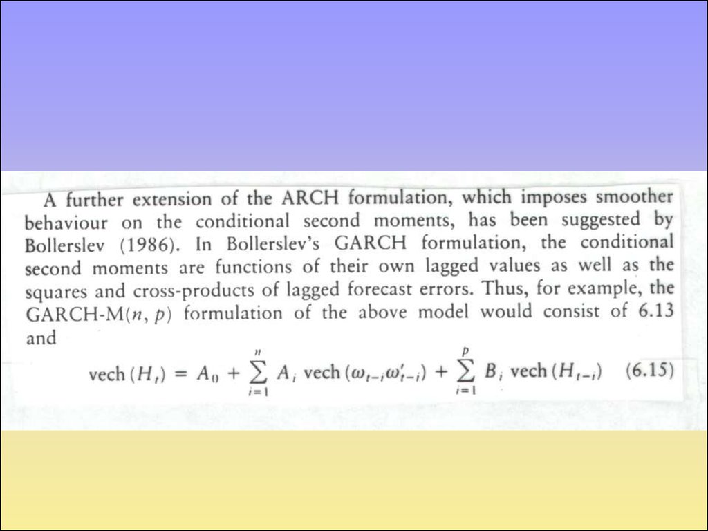
GARCH (Bollerslev(1986))
In empirical work with ARCH models high q is often required, a
more parsimonious representation is the Generalised ARCH model
q
p
i 1
j 1
2 t i 2 t i j 2 t j
( L) ( L)
2
define t t
2
2
2
t
t ( ( L) ( L)) ( L) t
2
2
which is an ARMA(max(p,q),p) model for the squared
innovations.

12.

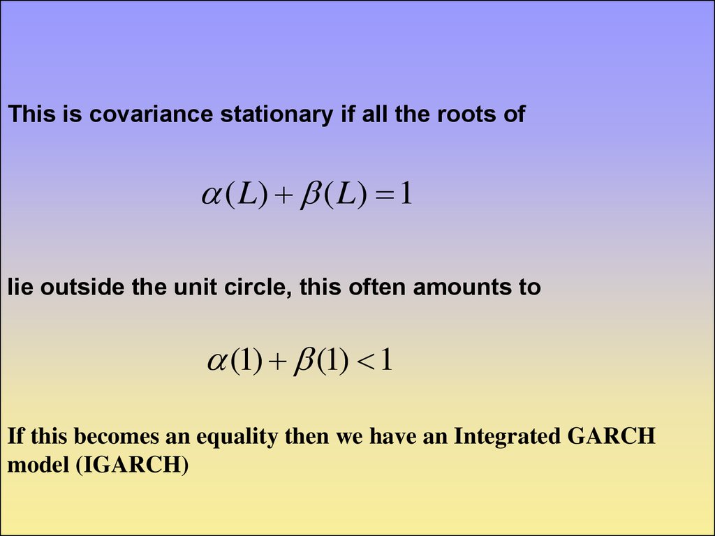
This is covariance stationary if all the roots of
( L) ( L) 1
lie outside the unit circle, this often amounts to
(1) (1) 1
If this becomes an equality then we have an Integrated GARCH
model (IGARCH)

13.

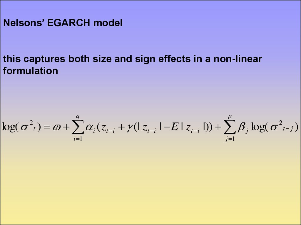
Nelsons’ EGARCH model
this captures both size and sign effects in a non-linear
formulation
q
p
i 1
j 1
log( 2 t ) i ( zt i (| zt i | E | zt i |)) j log( 2 t j )

14.

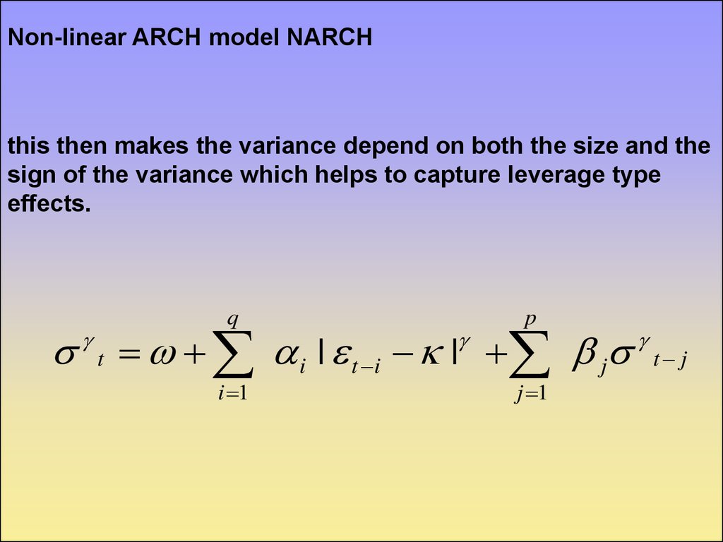
Non-linear ARCH model NARCH
this then makes the variance depend on both the size and the
sign of the variance which helps to capture leverage type
effects.
q
t
p
i | t i | j
i 1
j 1
t j

15.

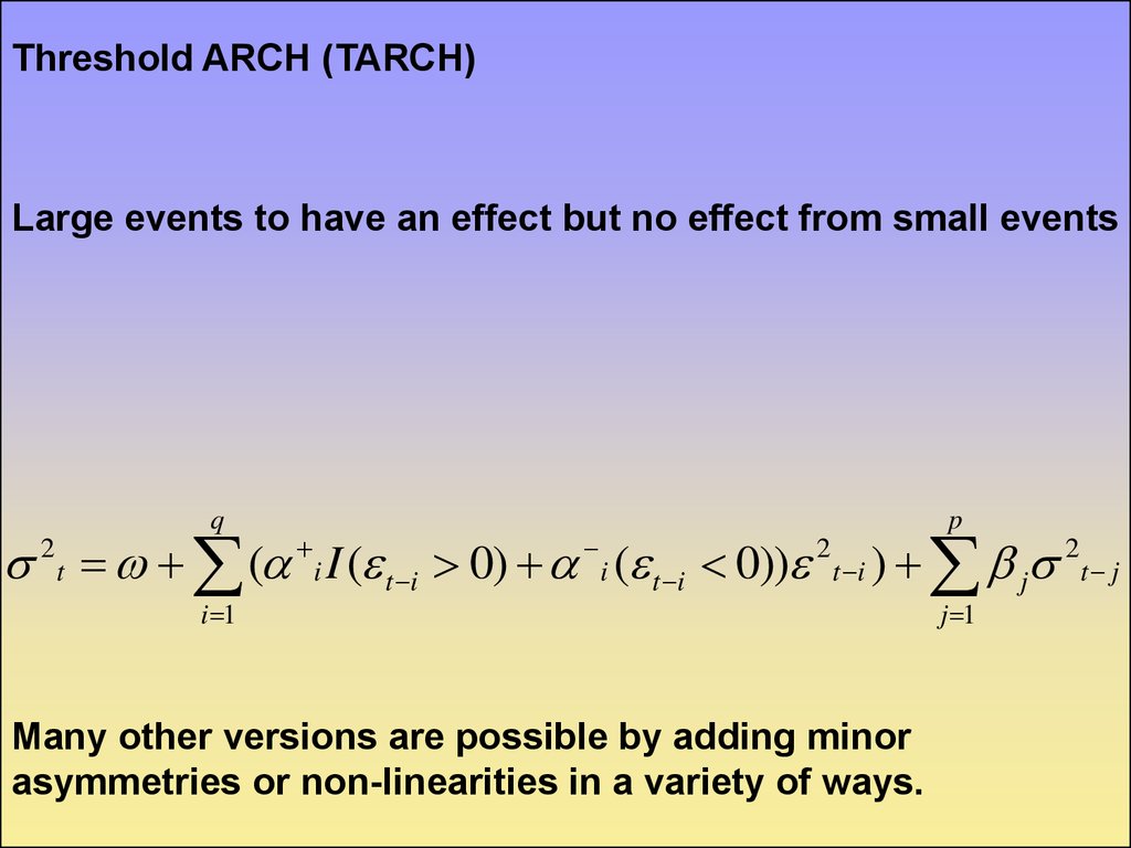
Threshold ARCH (TARCH)
Large events to have an effect but no effect from small events
q
t ( i I ( t i 0) i ( t i 0))
2
i 1
p
2
t i
) j
Many other versions are possible by adding minor
asymmetries or non-linearities in a variety of ways.
j 1
2
t j

16.

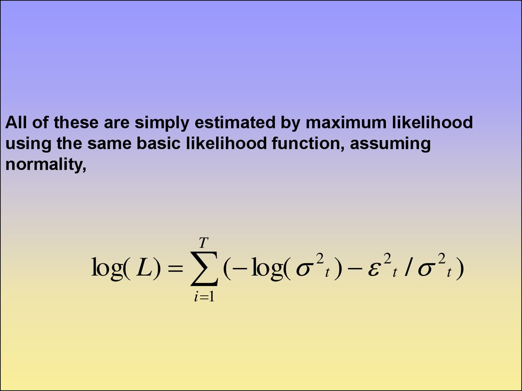
All of these are simply estimated by maximum likelihood
using the same basic likelihood function, assuming
normality,
T
log( L) ( log( t ) t / t )
2
i 1
2
2

17.

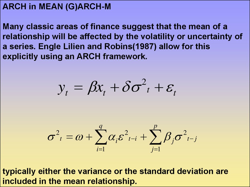
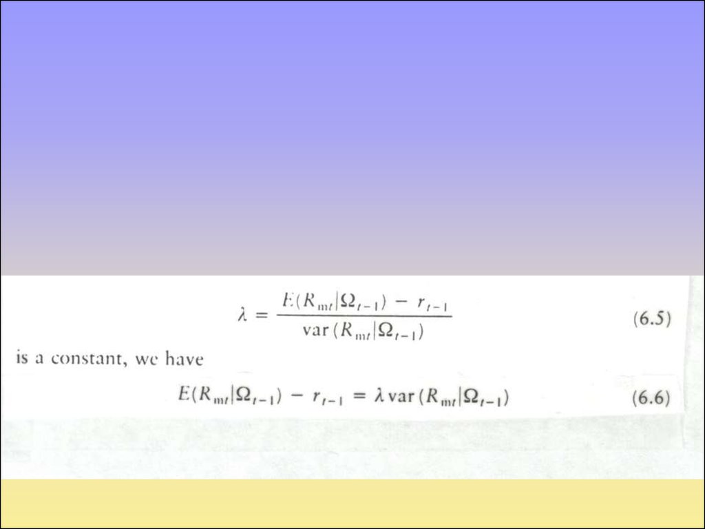
ARCH in MEAN (G)ARCH-M
Many classic areas of finance suggest that the mean of a
relationship will be affected by the volatility or uncertainty of
a series. Engle Lilien and Robins(1987) allow for this
explicitly using an ARCH framework.
yt xt t t
2
q
t i
2
i 1
p
2
t i
j
2
t j
j 1
typically either the variance or the standard deviation are
included in the mean relationship.

18.

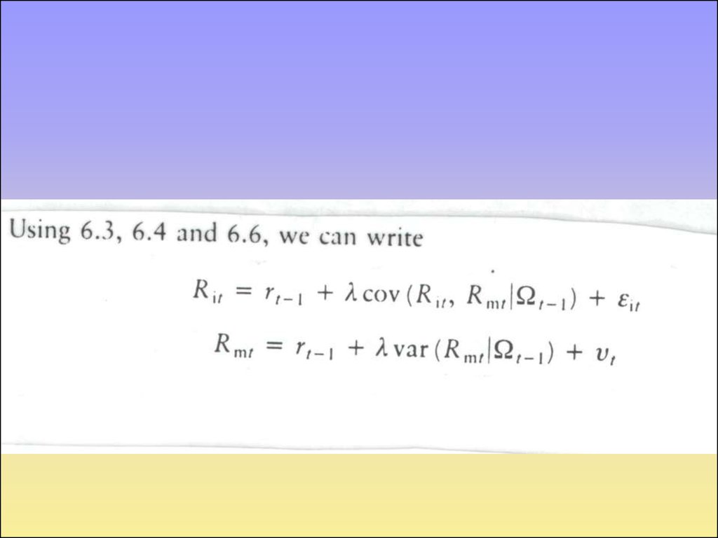
often finance stresses the importance of covariance terms.
The above model can handle this if y is a vector and we
interpret the variance term as a complete covariance matrix.
The whole analysis carries over into a system framework

19.

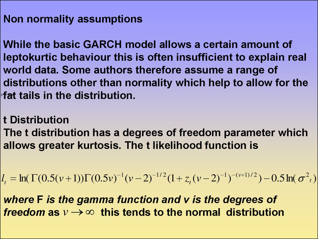
Non normality assumptions
While the basic GARCH model allows a certain amount of
leptokurtic behaviour this is often insufficient to explain real
world data. Some authors therefore assume a range of
distributions other than normality which help to allow for the
v
fat tails in the distribution.
t Distribution
The t distribution has a degrees of freedom parameter which
allows greater kurtosis. The t likelihood function is
lt ln( (0.5(v 1)) (0.5v) 1 (v 2) 1 / 2 (1 zt (v 2) 1 ) ( v 1) / 2 ) 0.5 ln( 2 t )
where F is the gamma function and v is the degrees of
freedom as v this tends to the normal distribution

20.

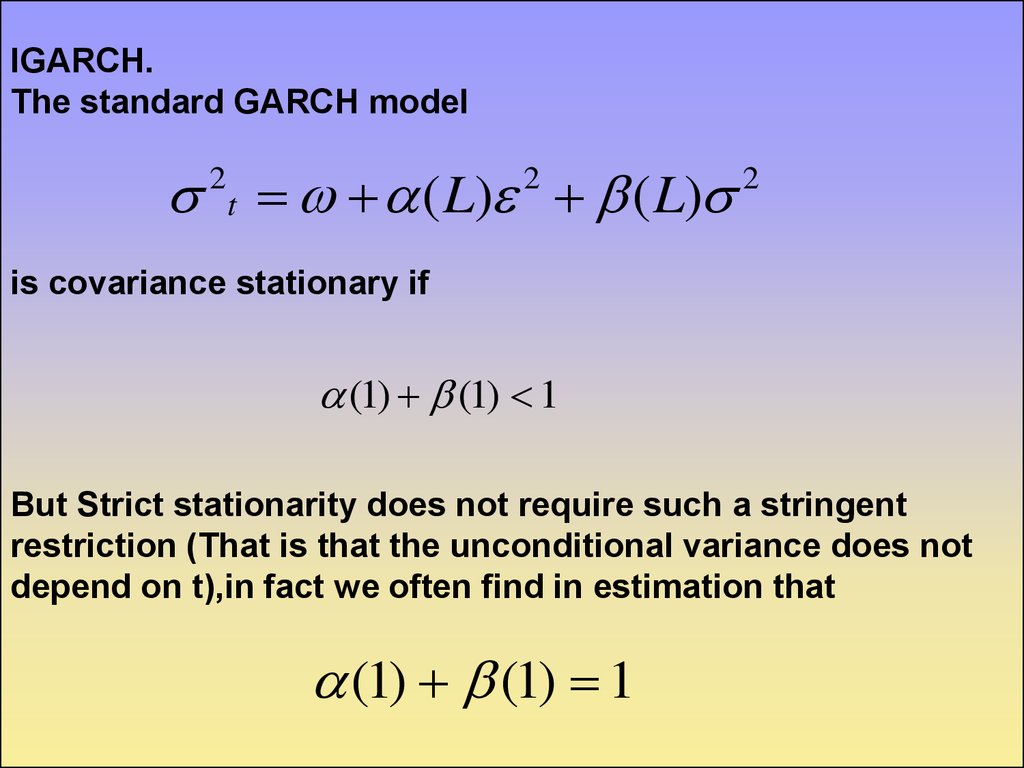
IGARCH.
The standard GARCH model
t ( L) ( L)
2
2
2
is covariance stationary if
(1) (1) 1
But Strict stationarity does not require such a stringent
restriction (That is that the unconditional variance does not
depend on t),in fact we often find in estimation that
(1) (1) 1

21.

this is then termed an Integrated GARCH model (IGARCH),
Nelson has established that as this satisfies the requirement
for strict stationarity it is a well defined model.
However we may suspect that IGARCH is more a product of
omitted structural breaks than the result of true IGARCH
behavior.

22.

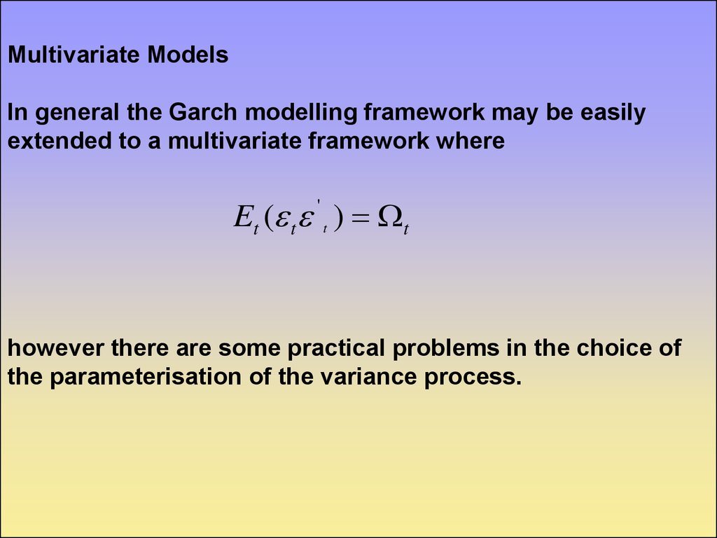
Multivariate Models
In general the Garch modelling framework may be easily
extended to a multivariate framework where
Et ( t ' t ) t
however there are some practical problems in the choice of
the parameterisation of the variance process.

23.

A direct extension of the GARCH model would involve a very
large number of parameters.
The conditional variance could easily become negative even
when all the parameters are positive.
The chosen parameterisation should allow causality between
variances.

24.

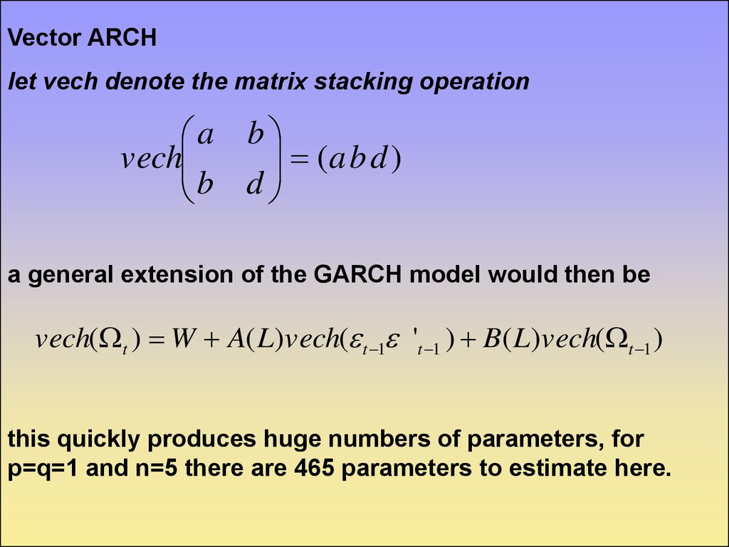
Vector ARCH
let vech denote the matrix stacking operation
a b
(a b d )
vech
b d
a general extension of the GARCH model would then be
vech( t ) W A( L)vech( t 1 't 1 ) B( L)vech( t 1 )
this quickly produces huge numbers of parameters, for
p=q=1 and n=5 there are 465 parameters to estimate here.

25.

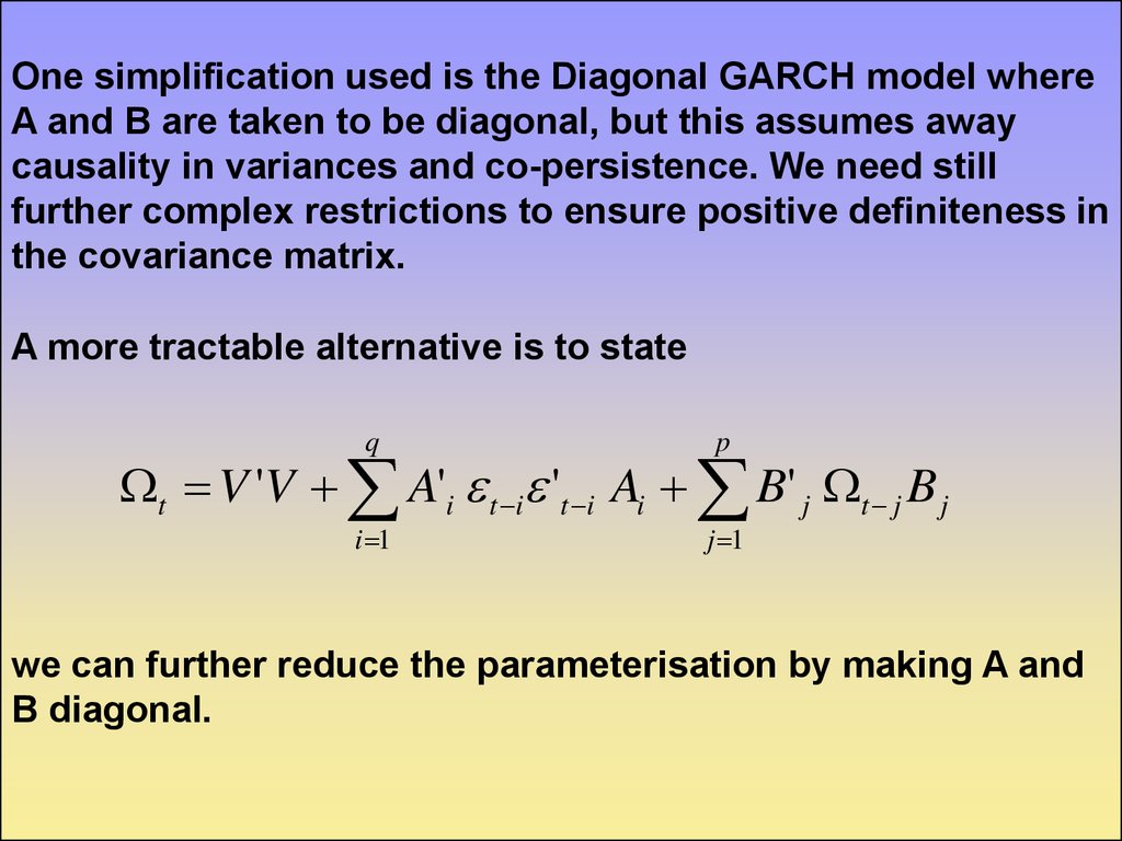
One simplification used is the Diagonal GARCH model where
A and B are taken to be diagonal, but this assumes away
causality in variances and co-persistence. We need still
further complex restrictions to ensure positive definiteness in
the covariance matrix.
A more tractable alternative is to state
q
p
i 1
j 1
t V 'V A'i t i 't i Ai B' j t j B j
we can further reduce the parameterisation by making A and
B diagonal.

26.

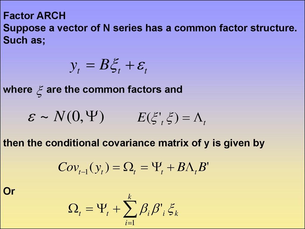
Factor ARCH
Suppose a vector of N series has a common factor structure.
Such as;
yt B t t
where
are the common factors and
~ N (0, )
E ( 't ) t
then the conditional covariance matrix of y is given by
Covt 1 ( yt ) t t B t B'
Or
k
t t i 'i k
i 1

27.

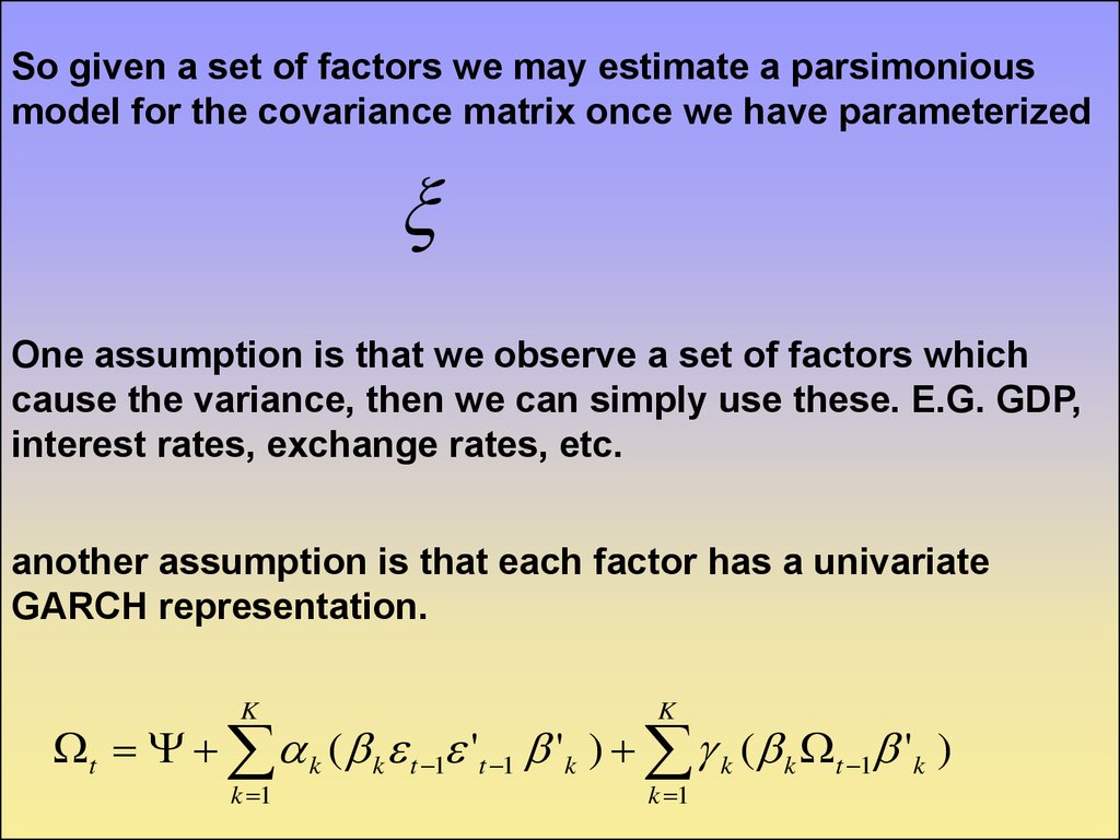
So given a set of factors we may estimate a parsimonious
model for the covariance matrix once we have parameterized
One assumption is that we observe a set of factors which
cause the variance, then we can simply use these. E.G. GDP,
interest rates, exchange rates, etc.
another assumption is that each factor has a univariate
GARCH representation.
K
K
k 1
k 1
t k ( k t 1 't 1 'k ) k ( k t 1 'k )