Similar presentations:
Lecture 1. Introduction to Econometrics
1. Elements of Econometrics. Lecture 1. Introduction.
ICEF, 2015-20162. The Subject of Econometrics
Econometrics is the application of statisticalmethods to the quantification and critical
assessment of hypothetical economic
relationships using data.
The Art of Econometrician: Finding the set of
assumptions which are sufficiently specific and
realistic in order to take the best possible
advantage from the data available.
(E.Malinvaud).
3. The Aims and Approaches of the Course
The aims of the course are:- To develop an understanding of the use of
regression analysis for quantifying economic
relationships and testing economic theories.
- To equip for reading and evaluation of empirical
papers in professional journals.
- To provide practical experience of using
econometric software to fit economic models
(Econometric Views will be used).
4. Methodology of Econometrics:
1. Statement of Theory or Hypothesis2.Specification of Mathematical Model
3. Specification of Econometric Model
4. Obtaining the Data
5. Estimation of the Parameters
6. Hypothesis Testing
7. Forecasting or Prediction
8. Using the Model for Control or Policy Purposes
5. Economic Relationships and Models Considered in the Course
-Demand and Supply functions;
Earnings functions;
Production functions;
Cost functions;
Economic growth models;
Educational attainment functions;
Consumption functions;
Investment functions;
Macroeconomic equilibrium models;
Academic success functions.
6. Econometric Analysis of ICEF Students UoL Exams Results
Elements of Econometrics, 2012-2014The model specification for 2012:
EOE_UOL = 4.01 + 0.51 EOE_ICEF + 0.38 MACMIC_UOL + e
(1.01)
(6.96)
(4.09)
(t-statistics are in parentheses; R2 = 0.76; 92 observations in the sample).
The model specification for 2013:
EOE_UOL = 7.79 + 0.44 EOE_ICEF + 0.56 MACMIC_UOL + e
(2.31)
(7.16)
(5.80)
(t-statistics are in parentheses; R2 = 0.70; 132 observations in the sample).
The model specification for 2014:
EOE_UOL = 6.36 + 0.35 EOE_ICEF + 0.59 MACMIC_UOL + e
(1.51)
(3.52)
(5.68)
(t-statistics are in parentheses; R2 = 0.61; 114 observations in the sample).
EOE_UOL – UoL exam grade in Econometrics,
EOE_ICEF – the average of ICEF Econometrics exams grades in October, December and
March,
MACMIC_UOL – the average of UoL grades in Micro- and Macroeconomics.
7. The Questions on the Model to be answered in the Course
Is the model specification reliable? How to interpret it?How to interpret the explanatory variables? Why and
how do they influence the UoL grades?
Does the model stay the same year by year? How to test
this?
Are there other factors missing, which ones, and how
does this influence the outcome?
Are there other links between the model variables?
Does it influence the conclusions?
Can we use the model for predictions?
8. Time Series Example: Price of Oil (Brent) and RuR/USD Exchange Rate (01/09/14-31/08/15)
110100
90
80
70
60
50
40
30
175
200
225
250
275
RUR_USD
300
325
350
375
400
OIL_BRENT
The relationship is available but there are questions to answer:
- Were there other factors to be included in the model?
- What was the time structure of the relationship (lags, trends, autocorrelations, etc)?
- Was the reaction the same or changed in time?
- Could the behaviour of the series in time (e.g. stationarity) influence the
conclusions?
9. Reading
Main Textbook:Dougherty, Christopher. Introduction to Econometrics. Oxford University Press, 2011,
2006 (4th or 3rd edition). Russian translation: Доугерти Кр. Введение в
эконометрику. Изд.3. М., ИНФРА-М, 2009.
Student resources for the book (Data sets, slides, Study Guide): VLE
Additional Textbooks:
Gujarati D.N. Basic Econometrics.
Wooldridge J.M. Introductory Econometrics. A modern approach.
Study Guides:
Dougherty, Christopher. Elements of econometrics. Study Guide. University of London.
2014.
ICEF materials: Lecture Notes, Slides, Class Notes, Exam Materials (ICEF Information
System).
Other reading: see the Course Syllabus, ICEF.
10. Main Electronic Resources:
ICEF Information System: http://icef-info.hse.ruUniversity of London site:
http://www.londoninternational.ac.uk/community/students
VLE Student Portal: http://my.londonexternal.ac.uk/london/portal
Course EC2020 Elements of econometrics
Oxford University Press: www.oup.com/uk/orc/bin/9780199567089
http://crow.academy.ru/econometrics - many useful materials
ICEF Computer Classes (desktops): «Хрестоматия по
Эконометрике»
11. Statistical Glossary for Econometrics:
Descriptive statistics: Mean, variance, standard deviation,
covariance, correlation
Random variables, Probability distributions: Discrete and
Continuous, Uniform, Normal, t-, F-, 2 - distributions. Expected
value, population variance and covariance. Independence.
Sampling : Population, sample. Sample selection.
Estimation: Estimator, estimate. Unbiasedness (expected value),
consistency (probability limit), efficiency. Central limit theorem.
Statistical Inference: Hypothesis testing. Significance tests,
significance levels. Power of a test, Type I and Type II errors. t-tests,
F-tests. Confidence intervals. P-values. One-sided and two-sided
tests.
Data types: Cross-section, time series, panel.
Rules: variance, covariance and probability limit rules.
12. Example: Plim rules
Plim rule 1
Plim rule 2
Plim rule 3
Plim rule 4
• Plim rule 5
• Plim rule 6
plim (X + Y) = plim X + plim Y
plim bX = b plim X
if b is a constant, plim b = b
plim Z = (plim X)(plim Y)
plim Z =
plim X
plim Y
plim f(X) = f(plim X)
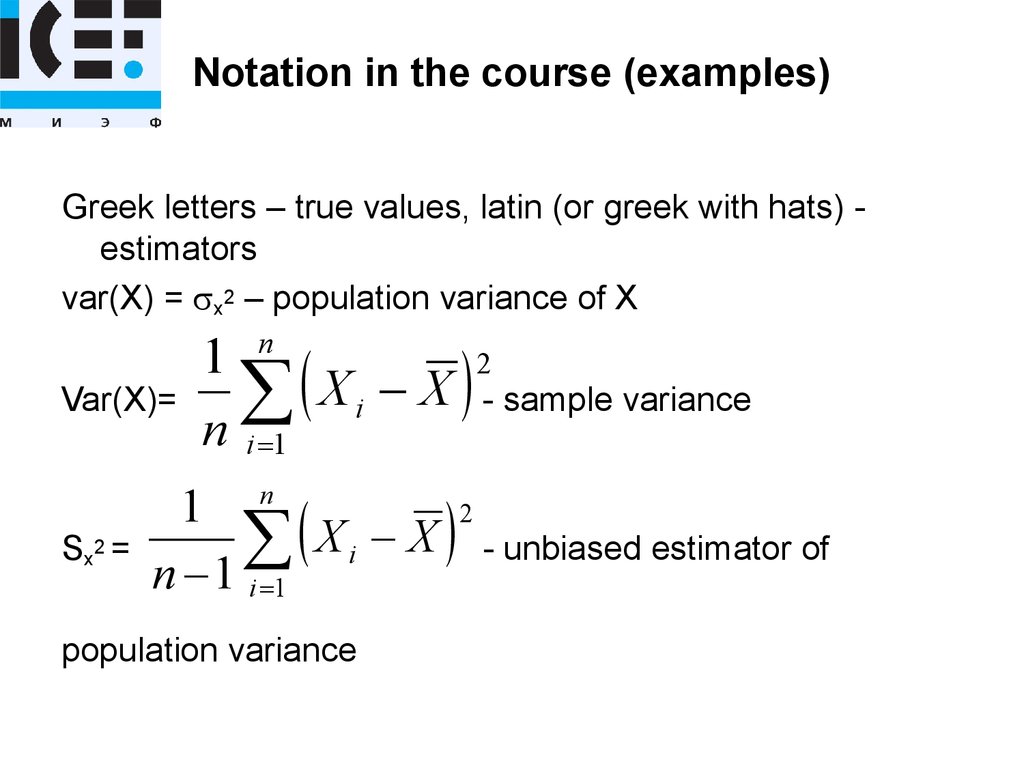
13. Notation in the course (examples)
Greek letters – true values, latin (or greek with hats) estimatorsvar(X) = x2 – population variance of X
Var(X)=
Sx2 =
1 n
2
X i X - sample variance
n i 1
1 n
2
X i X - unbiased estimator of
n 1 i 1
population variance
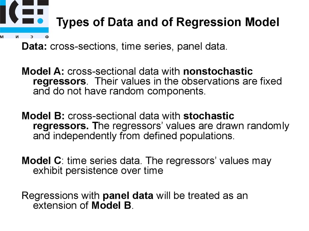
14. Types of Data and of Regression Model
Data: cross-sections, time series, panel data.Model A: cross-sectional data with nonstochastic
regressors. Their values in the observations are fixed
and do not have random components.
Model B: cross-sectional data with stochastic
regressors. The regressors’ values are drawn randomly
and independently from defined populations.
Model C: time series data. The regressors’ values may
exhibit persistence over time
Regressions with panel data will be treated as an
extension of Model B.
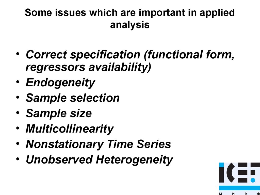
15. Some issues which are important in applied analysis
• Correct specification (functional form,regressors availability)
• Endogeneity
• Sample selection
• Sample size
• Multicollinearity
• Nonstationary Time Series
• Unobserved Heterogeneity
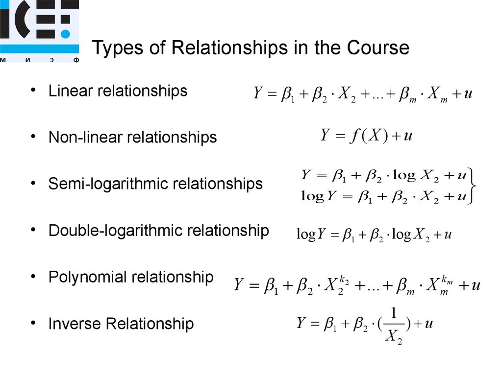
16. Types of Relationships in the Course
• Linear relationshipsY 1 2 X 2 ... m X m u
Y f (X ) u
• Non-linear relationships
• Semi-logarithmic relationships
Y 1 2 log X 2 u
log Y 1 2 X 2 u
• Double-logarithmic relationship
log Y 1 2 log X 2 u
• Polynomial relationship
• Inverse Relationship
Y 1 2 X 2k 2 ... m X mk m u
Y 1 2 (
1
) u
X2




 economics


