


 Diagram of Circular Flows")


")


")


 economics
 english
Similar presentations:


Introduction to macroeconomics (Lecture 1)
1. Macroeconomics
Lecturer – MATVEEVA Tatiana Yurievna2.
"The study of economics does not seem to require any specializedgifts of an unusually high order. Is it not, intellectually regarded, a
very easy subject compared with the higher branches of philosophy
and pure science? Yet good, or even competent, economists are the
rarest birds. An easy subject, at which very few excel! The paradox
finds its explanation, perhaps, in that the master-economists must
possess a rare combination of gifts. He must reach a high standard in
several different directions and must combine talents not often found
together. He must be mathematician, historian, statesman, philosopher
– in some degree. He must understand symbols and speak words. He
must contemplate the particular in terms of the general, and touch
abstract and concrete in the same flight of thought. He must study the
present in the light of the past for the purposes of the future. No part
of man's nature or his institutions must lie entirely outside his regard.
He must be purposeful and disinterested in a simultaneous mood; as
aloof and incorruptible as an artist, yet sometimes as near the earth as
a politician".
2
John Maynard Keynes
2
3.
33
4. Lecture 1 Introduction to Macroeconomics
The Subject Matter of Macroeconomics
The History of Macroeconomics
Key Macroeconomic Issues
Principles of Macroeconomic Analysis
Macroeconomic Agents and Macroeconomic
Markets
• The Model of Circular Flows
• The Macroeconomic System
4
5. What is Macroeconomics?
Macroeconomics is the branch of economics.Economics is a discipline which studies how scarce economic
resources are allocated and used to maximize production for a
society. It is a social science which deals with economic behavior
of individuals and organizations engaged in the production,
distribution and consumption of goods and services.
The study of economics is subdivided into two general fields:
Economics
Microeconomics
Macroeconomics
5
6. The History of the Term «Macroeconomics»
In translation from Greek«micro» means «small»,
«macro» – «large»;
аnd «ecоnоmics» – «housekeeping»
For the first time the term “macroeconomics” was used
in 1933 by the Norwegian economist-matematician
Ragnar Frisch (Nobel prize, 1969) who introduced the concepts
of “microeconomic” and “macroeconomic dynamics”.
In 1941 Piet De Wolff divided economic theory
into microeconomics and macroeconomics.
6
7.
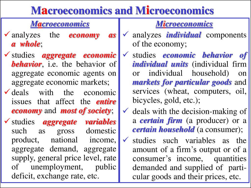
Macroeconomics and MicroeconomicsMacroeconomics
analyzes the economy as
a whole;
studies aggregate economic
behavior, i.e. the behavior of
aggregate economic agents on
aggregate economic markets;
deals with the economic
issues that affect the entire
economy and most of society;
studies aggregate variables
such as gross domestic
product, national income,
aggregate demand, aggregate
supply, general price level, rate
of unemployment, public
deficit, exchange rate, etc.
Microeconomics
analyzes individual components
of the economy;
studies economic behavior of
individual units (individual firm
or individual household) on
markets for particular goods and
services (wheat, computers, oil,
bicycles, gold, etc.);
deals with the decision-making of
a certain firm (a producer) or a
certain household (a consumer);
studies such variables as the
amount of a firm’s output or of a
consumer’s income, quantities
demanded and supplied of particular goods and their prices, etc.
8. Macroeconomics versus Microeconomics
MicroeconomicsMacroeconomics
Subject
Economic behavior
Economic behavior
Level of
analysis
Individual units
Entire economy
Agents
Individual
Aggregate
(sectors of economy)
Markets
Particular goods and
services
Composite
Prices
Relative
Absolute
Market
Adjustment
Only via changes
in prices
In the short run via
changes in quantities
8
9. Using Microeconomics in Macroeconomics
Macroeconomics is based on microeconomics(has microeconomic foundations), because
macroeconomic events are the result of the decisions
of millions of individual agents, maximizing their own
welfare and arise from the interaction of many people.
At the same time all the decisions of individual agents are
made taking into account the macroeconomic situation.
Microeconomics
Macroeconomics
9
10. Macroeconomics as a Special Discipline
But …despite
both
disciplines
use
the
same
variables,
macroeconomic variables are not just a simple sum of
variables that reflect individual decisions (examples: total output,
aggregate demand, general price level, etc);
not every statement that is true for an individual is always true
for the entire economy (example: the paradox of thrift).
Thus, microeconomics and macroeconomics have specific subjects
and methods of analysis and are based on specific approaches
and theories. They are even taught as separate disciplines.
10
11. The founder of macroeconomics as a special part of economics was a prominent British economist, lord John Maynard Keynes, who in 1936 published his famous book «General Theory of Employment, Interest and Money».
The Founder of MacroeconomicsThe founder of macroeconomics as a special part
of economics was a prominent British economist, lord
John Maynard Keynes,
who in 1936 published his famous book
«General Theory of Employment, Interest and Money».
He showed that macroeconomics
has a special subject and
some special methods of analysis.
His contribution to economic theory was
so large, that it was called the
«Keynesian revolution».
11
12. The History of Macroeconomics
The ХVIII century – beginning of the ХХ century – classical schoolin economic theory.
David Hume «Of the Balance of Trade», 1752 – the analysis of the
relation between the money stock, trade balances and the price level; laid
the foundation of the quantity theory of money.
The main ideas and concepts of the classical approach were
developed in the works of Adam Smith («An Inquiry into the Nature and
Causes of the Wealth of Nations», 1776), David Ricardo («On the
Principles of Political Economy and Taxation», 1817), Jean-Baptiste
Say («Traité d’économie politique ou Simple exposé de la manière dont
se forment, se distribuent et se consomment les richesses», 1803; «Cours
complet d’économie politique pratique», 1828–1830), William Stanley
Jevons («The Theory of Political Economy», 1871), Leon Walras
(«Elements of Pure Economics», 1874), Alfred Marshall («The
Principles of Economics», 1890), John Bates Clark («The Distribution
of Wealth», 1899), Arthur Pigou («The Economics of Welfare», 1920).
13. Classical Economists: the Gallery
David HumeAdam Smith
Marie-Ésprit-Léon
Walras
David Ricardo
Alfred Marshall
William Stanley
Jevons
John Bates
Clark
Jean-Baptiste
Say
Arthur Cecil
Pigou
13
14. Classical School: Basic Propositions
Economy consists of two separate sectors: the real sector andthe money sector real variables do not depend from
nominal variables = the principle of «classical dichotomy»
and «neutrality of money».
There is perfect competition in all the markets economic
agents cannot influence market prices, they are price-takers.
All the prices are flexible and are set by the relation between
supply and demand the principle of A.Smith’s «invisible
hand» and «market clearing».
Government has no need to intervene in the regulation of the
economy the principle «laissez faire, laissez passer».
14
15. Classical School: Basic Propositions
The main economic problem is the scarcity of resources, whichhence are fully used, and the economy is always at its potential
level of output.
The scarcity of resources poses puts in the forefront the problem
of production the analysis of economy’s behavior from
aggregate supply side («supply-side analysis»).
The «Say’s law» acts in the economy: «supply creates its own
demand», because each economic agent is simultaneously a seller
and a buyer.
The problem of expanding of production possibilities is resolving
slowly, the mutual market adjustment is a long-term process
the description of economy’s behavior in the long run («longrun analysis»).
15
16. The History of Macroeconomics
But up to the ХХ century macroeconomics didn’t exist as a separatediscipline.
Three events had the fundamental importance for the development of
macroeconomics:
the beginning of the collection of economic information and
systematization of aggregate data (the period of the I World War)
that provided the empirical base for macroeconomic research:
1920-s – the elaboration of the System of National Income and
Product Accounts (NIPA) – Simon Kuznets (Nobel prize, 1971)
and Richard Stone (Nobel prize, 1984);
the substantiation of the fact that the business cycle is a recurring
phenomenon (1920-s – Wesley Clair Mitchell );
the Great Depression (1929–1933) – world economic catastrophe
(the Great Crash) that contradicted to the postulates of classical
16
economists about the self-correcting economy.
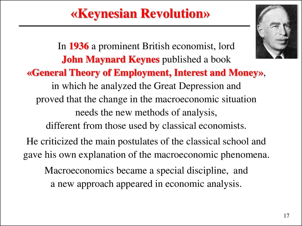
17.
«Keynesian Revolution»In 1936 a prominent British economist, lord
John Maynard Keynes published a book
«General Theory of Employment, Interest and Money»,
in which he analyzed the Great Depression and
proved that the change in the macroeconomic situation
needs the new methods of analysis,
different from those used by classical economists.
He criticized the main postulates of the classical school and
gave his own explanation of the macroeconomic phenomena.
Macroeconomics became a special discipline, and
a new approach appeared in economic analysis.
17
18. Keynes’ Approach: Basic Propositions
The real sector and the money sector are related to each othermoney affect real variables, the interest rate is set in the
money market rather than in the loanable funds (or capital) market.
There is imperfect competition in the markets.
Prices (nominal variables) are rigid («sticky»).
Equilibrium in the markets is settled, but not on the full-employment
level.
Private sector expenditures are unable to provide the level of
aggregate demand required to obtain the potential level of output, and,
therefore, government intervention and government regulation is
needed.
In the conditions of underemployment of economic resources
aggregate demand becomes the main problem of the economy
(«demand-side analysis»).
Government stabilization policy affects economy in the short run, and
price rigidity exists relatively for not long period the description of
18
the economy’s behavior in the short run («short-run analysis»).
19.
The History of MacroeconomicsThe central point of Keynes’ theory: the market economy does not
guarantee the economy’s stability, and, therefore, to counteract
slumps and recessions and high unemployment government
should intervene in the economic performance and conduct the
stabilization policy.
During 25 years after the II World War – the period of fast
economic growth in most countries – the belief that government
is able to prevent recessions by actively using fiscal and
monetary policy.
But in the middle of 1970-x – stagflation (the combination of high
inflation with stagnation, i.e. low and even negative rates of
economic growth and high unemployment) – the conclusion: the
key source of instability is the stabilization policy itself
«Neoclassical counterrevolution».
19
20. Schools Alternative to Keynesian Approach
Monetarism (Milton Friedman, Edmund Phelps )- the market economy is a self-correcting system and is able to return
to the potential level of output by itself;
- economic fluctuations are the result of the changes in the money
stock, therefore, to provide stability the Central bank should maintain
the constant money growth rate («monetary rule»);
New Classical Macroeconomics (Robert Lucas, Thomas Sargent,
Neil Wallace) (the rational expectations theory)
- if the economic agents’ expectations are rational, government policy
is ineffective;
Real Business Cycle Theory (Finn Kydland, Edward Prescott)
- the source of economic disturbances are technological shocks rather
than government policy.
Supply-side Economics (Arhur Laffer)
- government policy should be aimed to stimulate aggregate supply
rather than aggregate demand.
20
21. Schools Alternative to Keynesian Approach: the Gallery
MonetarismMilton Friedman,
Nobel prize, 1976
Edmund Phelps,
Nobel prize, 2006
Real Business Cycle Theory
Edward Prescott,
Nobel prize, 2004
New Classical Macroeconomics
Robert Lucas,
Nobel prize, 1995
Thomas Sargent, Neil Wallace
Nobel prize, 2011
Finn Kydland,
Nobel prize, 2004
Supply-side Economics
Arthur Laffer
21
22. Development of Macroeconomics
Macroeconomics as a science is permanently developingchanges concern both the sense of issues and problems under
study and of answers and remedies proposed.
These changes are the result of the impact of two groups of factors:
The appearance of new theories,
while old theories are rejected as
not consistent with economic
reality or as outdated in the light
of new concepts.
The permanent
development of the
economy itself,
that poses new questions
and requires new answers.
22
23. Diversity of Macroeconomic Theories
The diversity of approaches to the explanationof macroeconomic events and especially
problems of macroeconomic policy is caused
by the fact that different groups of
macroeconomists construct their theories by
using different assumptions, may differently
interpret the same events, and therefore, come
to different theoretical and practical
conclusions
and give different political
recommendations.
This diversity of ideas is due to the
complexity of macroeconomic problems and
allows to examine them comprehensively,
thoroughly, and from different points of view.
23
24. Key Questions Macroeconomists Try to Answer
??
Why do incomes grow? Would our children live better than we do?
Why are some countries richer than others? Why do some
countries are growing faster than others?
?
Why recessions and expansions occur in the economy?
?
Why is there unemployment? Is it a necessary part of economic
life? Why unemployment is low in some countries and high in the
others?
?
Why prices grow? What is the cost of inflation for the society?
Is it better for an economy to have budget deficit or budget
surplus? trade deficit or trade surplus? to be a lender or a borrower
in the world financial markets?
?
?
24
25. Questions Macroeconomists Try to Answer
Why interest rates fluctuate? What impact have the changesin the money and stock markets on the economy?
?
?
What are the determinants of the exchange rates? Is it good
to have a strong or a weak domestic currency?
?
Is government policy able to affect long-term economic
growth? Can it eliminate or at least smooth economic
fluctuations during the business cycle?
?
?
How economic changes in one country effect the situation
in others?
?
Answer: study macroeconomics and be informed!
25
26. Key Macroeconomic Issues
Overall output- long-run changes – economic growth
- short run fluctuations – business cycle
Unemployment
Inflation
Interest Rates
Government Budget
Balance of Payments and Exchange Rates
Macroeconomic Policy
?
26
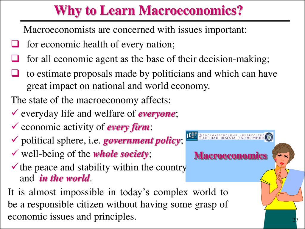
27.
Why to Learn Macroeconomics?Macroeconomists are concerned with issues important:
for economic health of every nation;
for all economic agent as the base of their decision-making;
to estimate proposals made by politicians and which can have
great impact on national and world economy.
The state of the macroeconomy affects:
everyday life and welfare of everyone;
economic activity of every firm;
political sphere, i.e. government policy;
well-being of the whole society;
Macroeconomics
the peace and stability within the country
and in the world.
It is almost impossible in today’s complex world to
be a responsible citizen without having some grasp of
economic issues and principles.
27
28. The Importance of Macroeconomics
Macroeconomic theoryreveals and explores the regularities of macroeconomic processes
and events;
aims to explain macroeconomic phenomenon;
helps to understand the cause-and-effect relations in the aggregate
economy;
serves the base for elaboration of principles, tools and measures of
macroeconomic policy that might prevent or improve economic
performance and can in the best way serve to the needs of the society;
provides the framework to make forecasts of future economic
development, to predict future economic problems.
Macroeconomics
a fascinating intellectual
great practical
represents
occupation that has
importance.
28
29. Principles of Macroeconomic Analysis
Macroeconomics is the social science and the controlled experimentis impossible. Besides, economic phenomena are very complex.
That’s why economists use models.
Economic model is a stylized representation of the economy, a
generalization and abstraction of reality that seeks to isolate a
few of the most important determinants (causes) of an economic
event in order to provide a better understanding of that event.
Economic models are constructed and used
to simplify the analysis of complex economic reality;
to examine the relationship between economic phenomena and
the regularity of their development;
to understand what goes on in the economy and how the
economy works;
to develop policies that might prevent, correct, or alleviate
economic problems and improve the situation in the economy;
29
to forecast future development of economic process.
30. Macroeconomic Models
To study the most important elements that explain how the wholeeconomy works, economic models are based on assumptions, which
cut off details unimportant for the analysis of a certain economic
process or phenomenon and reduce the complexity of economic
behavior.
Once modeled, economic behavior may be presented as a
relationship between a dependent (endogenous) variable and a few
independent (exogenous) variables.
Exogenous (independent) variable
is the one whose value is determined
by forces outside the model.
Endogenous (dependent)
variable is those whose value is
determined within the model.
The value of endogenous variable depends and is determined by
the value of exogenous variables.
Exogenous
MODEL
Endogenous
30
31.
The Rules of Model ConstructionFrequently, the endogenous variable is presented as depending
upon only one exogenous variable, with the assumption that all
the other exogenous variables are held constant. This principle
is called by the Latin term ceteris paribus, meaning «other
things being equal».
Models should be simple and focused on the examination of the
phenomenon or process under study. They do not need to be
«realistic», but should be consistent with the facts.
There must be the possibility of the transition from one model
to the other depending on the context.
There can be no one grand «true» model that exactly and
completely describes the economic reality.
31
32. Types of Relationship between Variables
An economic model specifies whether the dependent andindependent variables are positively or negatively related.
The relationship between
variables is positive when the
dependent variable moves in
the same direction as the
independent variable.
The relationship is negative when
the value of the dependent variable
increases (decreases) when the
value of the independent variable
decreases (increases).
Example: positive relation
of consumption spending
from income.
Example: negative relation
of investment spending
from the interest rate.
Models which specify economic reality provide the framework
for organizing data, empirically testing economic hypotheses,
and forecasting economic behavior.
32
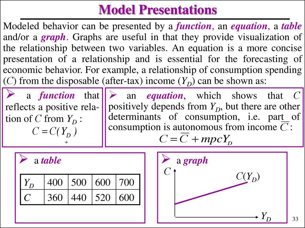
33.
Model PresentationsModeled behavior can be presented by a function, an equation, a table
and/or a graph. Graphs are useful in that they provide visualization of
the relationship between two variables. An equation is a more concise
presentation of a relationship and is essential for the forecasting of
economic behavior. For example, a relationship of consumption spending
(С) from the disposable (after-tax) income (YD) can be shown as:
a function that an equation, which shows that С
reflects a positive rela- positively depends from YD, but there are other
determinants of consumption, i.e. part of
tion of С from YD :
consumption is autonomous from income С :
С С( Y )
D
YD
C
a table
С С mpcYD
С
400 500 600 700
360 440 520 600
a graph
С(YD)
YD
33
34. Importance of Using Graphs
«Graphs are plotted by economiststo confuse students».
A student joke
A graph is a way of:
visual presentation of the relationship and links between
economic variables or of the behavior of a variable over time;
visual demonstration of ideas and theories, which are less clear
and even may be misinterpreted or misunderstood, when are only
verbally explained;
visual illustration of models proposed by economists.
In the course of economics graphs are used for the
better perception of theoretical propositions by students.
34
35.
Types of Visual Data PresentationTime Series Graph
Pie Diagram
Structure of Consumption Spending, Russia, 2012
Consumption
spending on
food goods – 33,8%
Consumption
spending on
nonfood goods – 38,6%
Consumption
spending on
services – 27,6%
Bar Diagram
10.0
Scatter Graph
GDP Growth Rate in Selected Countries
Investment Demand Curve
8.0
Interest
rate (r)
6.0
4.0
2.0
0.0
-2.0
1994 1995 1996 1997 1998 1999 2000 2001 2002 2003 2004 2005
I(r)
-4.0
-6.0
-8.0
-10.0
Luxembourg
United States
Japan
Investment (I)
35
35
36. Types of Analysis
Economic analysis is the combination of:functional (algebraic) analysis;
graphical (visual) analysis;
intuitive (substantial verbal) analysis.
In our course of macroeconomics the intuitive analysis (intuition)
will be of primary importance, because the main goal of the
economist is not simply to declare relations between
macroeconomic phenomena, but first of all and what is more – to
explain its economic sense.
Intuitive analysis assumes the study and the
explanation of the mechanism of macroeconomic
phenomena, the construction of logical chains of
the sequence of macroeconomic events, i.е.
examination and substantiation of the effect of one
event (or the change in one variable) on the other,
which in turn leads to further changes.
36
37. Algebraic and Graphical Analysis: Correlation
For simplicity sake in our analysis we will use the assumption aboutlinear relationship between variables that can be represented by
the following equations:
y = a + bx
or
y = a – bx
where
y – an endogenous (dependent) variable, which is plotted on one of
the axes of the scatter graph, i.e. it is a consequence;
x – an exogenous (independent) variable, which is plotted on the
other axis of the scatter graph, i.e. it is a cause or a determinant; its
change leads to the movement along the line;
a – an autonomous variable, which incorporates all the other
variables that affect an endogenous variable, and which can be
represented as a point of intersection of the line with the axis; its
change results in the parallel shift of the line;
37
38. Algebraic and Graphical Analysis: Correlation
Consumption lineС С mpcYD
С
mpc
Disposable Income (YD)
Investment line
Interest rate (i)
Consumption (С)
signs «+» or «–» characterize the type of the relationship between
exogenous and endogenous variable (positive or negative,
respectively) that is represented by the positive or negative slope
of the line;
b – the sensitivity (the extent of reaction) of the endogenous
variable to the change of the exogenous variable, measured as the
y
tangent of the angle (b ) ; its change results in the change of
x
the slope of the line.
I I bi
1
b
Investment (I)
I
38
39. Positive and Normative Economics
Positive Economic Theoryis the objective or scientific
attempt to describe and explain
the behavior of the economy
and its important variables;
reflects facts and studies
actual economic performance;
is an explanation why the
economy works as it does;
is a basis for predicting how
the economy will respond to
changes in circumstances;
free from subjective value
judgments;
represents an approach of a
scientist.
Normative Economic Theory
involves subjective value judgments
about what economy must be or what
measure is to be undertaken on the
base of a particular economic concept
or theory;
makes prescriptions what should be
done in the economy;
offers recommendations for changes in economic policy to achieve an
optimal and desirable state of affairs;
is based on personal (subjective)
value judgments;
represents an approach of a
39
politician.
40. The Model of Supply and Demand
This is the basic economic model. It describes the ubiquitous relationshipbetween buyers (demanders of goods and services, or consumers) and
sellers (suppliers of production, or producers) in the market and serves
to determine market equilibrium. Equilibrium is the state in the market
when the quantity that consumers wish to purchase exactly equals the
quantity producers wish to supply, and there is no pressure for change.
Geometrically it is the point of intersection of the market demand
curve (D) with the market supply curve (S). The price and the quantity
that equate quantity demanded with quantity supplied, are known,
respectively, as the equilibrium price and the equilibrium quantity.
Supply
Demand
Price (P)
Supply (S)
Equilibrium
price (PE)
E
Equilibrium
quantity (QE)
Equilibrium:
Quantity Demanded =
Quantity Supply
Demand (D)
Quantity (Q)
40
41. How Market Equilibrium is Reached
When there is the disequilibrium, and the price is equal either to P1that is higher than PE, or to P2 that is lower than PE, the price will
start to change in order to equate the quantity demanded by the buyers
with the quantity supplied by the producers.
Under the price P1, the quantity
Demand
supplied exceeds
the quantity
demanded = excess supply
(= a surplus = AB) the price
will fall to the equilibrium price PE.
Price (P)
P1
Supply (S)
Surplus
A
PE
P2
Under the price P2, the quantity
demanded exceeds the quantity
supplied = excess demand
Supply
(= a shortage
= CD) the price
will rise to the equilibrium price PE
E
B
D
C
Shortage
QE
The process is called
market clearing.
Demand (D)
Quantity (Q)
41
42. Market Clearing
Market clearing is an alignment process whereby decisions betweensuppliers and demanders reach an equilibrium.
When there is the change either in the market demand,
or in the market supply, the new equilibrium in the market
will be attained via price adjustment.
Suppose a sudden
increase in Suppose a sudden increase in
Demand
demand excess demand supply excess supply, on the
places a upward pressure on the contrary, places a downward
Supply
price from point A to point B pressure on the price and the new
since the original price Р1 no equilibrium price will be Р2.
longer clears the market.
In both cases market clears by itself.
S
S1
Price (P)
Price (P)
В
S2
Surplus
P2
P1
А
D2
Shortage
Q1 Q2
D1
Quantity (Q)
P1
P2
А
В
D
42
Q1 Q2 Quantity (Q)
43. Prices: Flexible versus Sticky
Economists typically assume that the market will go into anequilibrium of supply and demand.
But, assuming that markets clear continuously is not
realistic. For markets to clear continuously, prices would
have to adjust instantly to changes in supply and
demand, i.e. must be fully flexible.
But, evidence suggests that prices and wages often adjust
slowly and in actuality, some of them are sticky.
The difference between macroeconomic theories is
primarily based on the assumption of how quickly the
prices change and thus how quickly all the markets clear.
.
43
44. Long-run and Short-run Analysis
Time factor is of great importance in macroeconomics.Macroeconomists usually distinguish the short-run
and the long-run behavior of aggregate economy.
Long-run issues are analyzed under the assumption of flexible
prices (market clearing). The level of output is determined by the
amount of all available economic resources and by the existing in
the economy technology (i.e. by the production function or
aggregate supply). Such level is called potential output. Its changes
are associated with the long-run economic growth.
Short-run issues are analyzed under the assumption of rigid
(or sticky) prices. The level of output is mainly determined by the
aggregate expenditures in the economy (or aggregate demand).
Such level is called actual output. Its changes are associated with
the business cycle.
44
45. Long-run Growth versus Business Cycle
AggregateOutput
Economic Growth
(potential output)
Business Cycle
(actual output)
Time (years)
45
46. Types of Economic Resources
The amount of output that can be produced in the economy isdetermined by the quantity, quality and productivity of economic
resources, or factors of production, that are commonly separated
into four groups:
Labor: the physical and mental effort of people. This can be
increased by education, training and experience (human capital);
Physical capital: the stock of manmade equipment (like machinery,
tools, vehicles, computers) and structures (buildings, constructions,
real estate) that are used to produce goods and services;
Land or Natural resources: inputs provided by nature, such as
land, rivers, mineral deposits, oil and gas reserves. They come in
two forms: renewable and non-renewable.
Entrepreneurial ability: the ability to identify opportunities and
organize production (that is the effort and know-how to put the
other resources together in a productive venture), and the
46
willingness to accept risk in the pursuit of rewards.
47. Time Intervals in Macroeconomics
Olivier Blanchard in his textbook distinguishesthree time periods:
Short-run
Long-run
Medium-run
the analysis of what
the analysis of what
the analysis of what
happens in the
happens in the economy happens in the economy
economy
during approximately
during 50 years and
from year to year
one decade
more
According to these time intervals the accent is put
on the study of different macroeconomic problems, and
the analysis is based on different models.
47
48. Aggregation
The main principle of macroeconomic analysis is aggregation.Aggregation means putting all the units together.
The subject matter of macroeconomics is to study
aggregate economic behavior, i.e. behavior of
aggregate (macroeconomic) agents on
aggregate (macroeconomic) markets.
There are four macroeconomic agents and
four macroeconomic markets.
48
49. Macroeconomic Agents
Householdsthe owners of economic resources
(suppliers of factors of production);
the earners of national income;
the main consumers of goods and services
(demanders for aggregate output);
the main savers (lenders).
Firms
the main producers of goods and services
(suppliers of aggregate output);
the main demanders for economic resources;
the consumers of the part of aggregate output
(demanders for investment goods);
the main borrowers.
Households and firms form the private sector of the economy. 49
50. Macroeconomic Agents
Governmentthe producer of public goods;
the consumer of the part of aggregate output
(purchaser of goods and services);
the redistributor of national income (through collecting taxes and
making transfer payments);
lender or borrower in the financial markets (depending on the state
of government budget);
the regulator of economic activity:
- establishes and supports institutional basis for the economic
performance (“rules of the game”);
- conducts macroeconomic policy.
Private and government sectors form
the closed economy
(or the mixed closed economy), that is
the economy not interacting with other economies.
50
51.
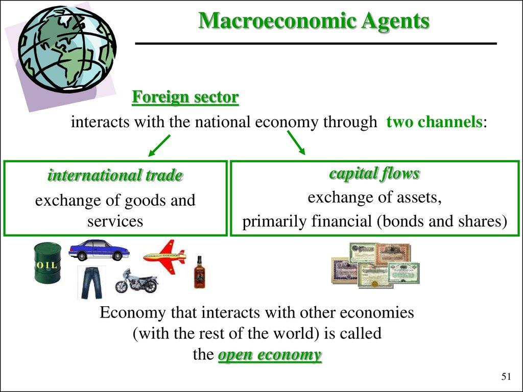
Macroeconomic AgentsForeign sector
interacts with the national economy through two channels:
international trade
exchange of goods and
services
capital flows
exchange of assets,
primarily financial (bonds and shares)
OIL
Economy that interacts with other economies
(with the rest of the world) is called
the open economy
51
52. Macroeconomic Markets
Goods (or product) marketResource (or factor) market
Financial market
which consists of two segments:
money market
bonds market
Foreign exchange market
Price (P)
Equilibrium
price (PE)
Supply (S)
E
Equilibrium:
Demand = Supply
Demand (D)
Equilibrium
quantity (QE)
Quantity (Q)
52
53. Model of Circular Flows
In order to understand how the aggregateeconomy works and to analyze the aggregate
economic behavior economists use
the model of circular flows, that represents
the interaction between macroeconomic
agents through macroeconomic markets.
We begin with the simple or private or two-sector model,
consisting of two macroeconomic agents
(households and firms)
and two macroeconomic markets
(goods market and resource market).
53
54. Simple (Private Sector) Diagram of Circular Flows
ExpendituresGoods and
Services Purchased
Revenues
Goods
Market
Goods and
Services Sold
Households
Firms
Land, Labor, Capital,
Inputs
Entrepreneurship Resource (Factor Services)
Incomes
Market
Factor Payments
(Wages, Rents,
Interest, Profits)
Flow of money
Flow of goods and services and of
economic resources
54
55. Private Sector Model of Circular Flows
Goods flow from firms to households through the goods (product)market and economic resources flow from households to firms
through the resource (factor) market.
Firms pay factor incomes (wages, rent, interest and profits) to
households - the owners of economic resources and households
spend their incomes buying goods and services. Hence,
• aggregate income is equal to aggregate expenditures
(all income is spent, all expenditures translate in somebody’s
income);
• aggregate expenditures are equal to aggregate product
• aggregate product is equal to aggregate income.
Movement of income, expenditures and product form a circle.
Thus, we have circular flows.
55
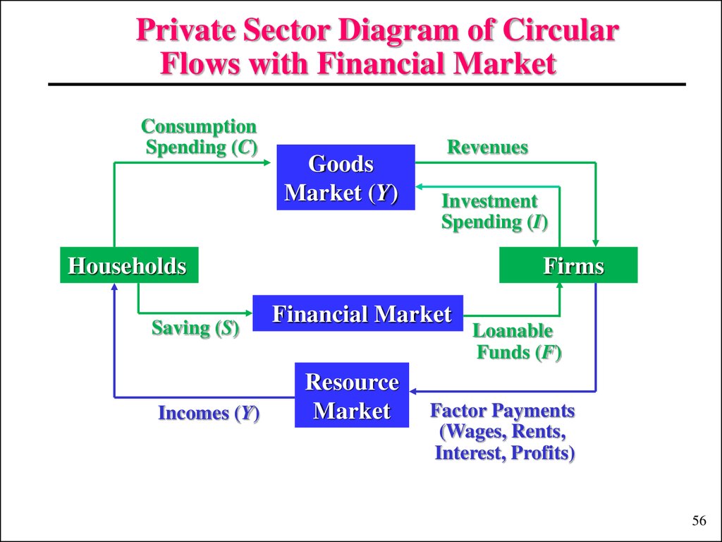
56.
Private Sector Diagram of CircularFlows with Financial Market
Consumption
Spending (C)
Goods
Market (Y)
Revenues
Investment
Spending (I)
Households
Saving (S)
Incomes (Y)
Firms
Financial Market
Resource
Market
Loanable
Funds (F)
Factor Payments
(Wages, Rents,
Interest, Profits)
56
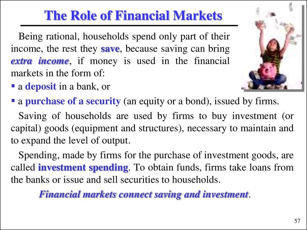
57.
The Role of Financial MarketsBeing rational, households spend only part of their
income, the rest they save, because saving can bring
extra income, if money is used in the financial
markets in the form of:
a deposit in a bank, or
a purchase of a security (an equity or a bond), issued by firms.
Saving of households are used by firms to buy investment (or
capital) goods (equipment and structures), necessary to maintain and
to expand the level of output.
Spending, made by firms for the purchase of investment goods, are
called investment spending. To obtain funds, firms take loans from
the banks or issue and sell securities to households.
Financial markets connect saving and investment.
57
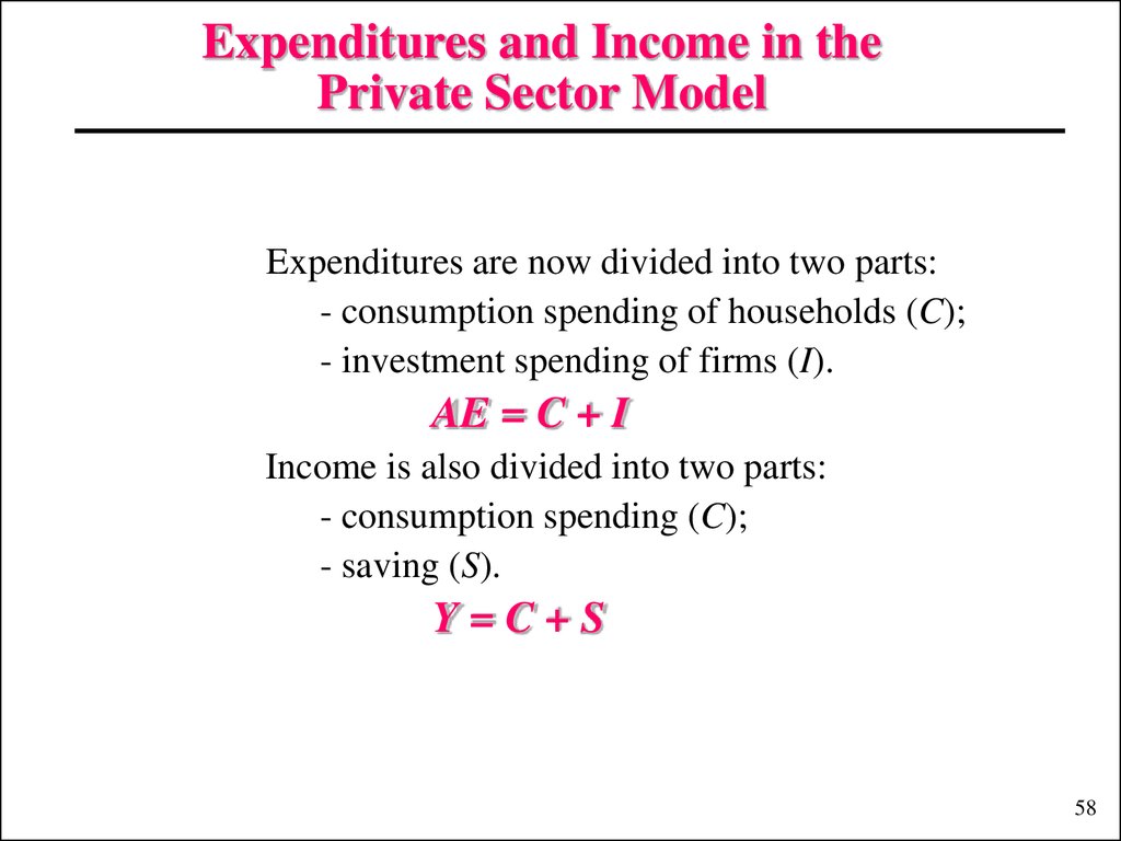
58.
Expenditures and Income in thePrivate Sector Model
Expenditures are now divided into two parts:
- consumption spending of households (C);
- investment spending of firms (I).
AE = C + I
Income is also divided into two parts:
- consumption spending (C);
- saving (S).
Y=C+S
58
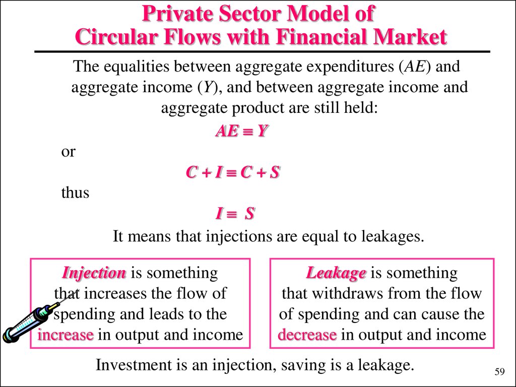
59.
Private Sector Model ofCircular Flows with Financial Market
The equalities between aggregate expenditures (AE) and
aggregate income (Y), and between aggregate income and
aggregate product are still held:
AE Y
or
C+I C+S
thus
I S
It means that injections are equal to leakages.
Injection is something
that increases the flow of
spending and leads to the
increase in output and income
Leakage is something
that withdraws from the flow
of spending and can cause the
decrease in output and income
Investment is an injection, saving is a leakage.
59
60. The Role of the Government
Adding government to our analysis, we get a three-sector model.The influence of the government sector is executed through:
Purchases of goods
and services (G)
which include:
goods purchased to
run government and
the military;
payments
to
govern-ment
employees and the
military for their
Transfers to households
(Tr) & subsidies
to firms (Sb)
which are government
payments that involve no
direct service by the
recipient. Transfers include:
unemployment insurance
payments;
welfare payments to
households.
In addition to transfers
persons receive interest on
public debt (i × BGov).
Taxes (Tx)
which are imposed
upon property
and income (direct
taxes);
upon goods and
services (indirect
taxes, such as VAT,
sales and excise
taxes)
in order to pay
for
all
the
expenditures of the
government.
60
61. Diagram of Circular Flows with Government (Mixed Closed Economy)
ConsumptionSpending (C)
Revenues
Goods
Market (Y)
Government
Taxes (Tx) Purchases (G)
Investment
Spending (I)
Taxes (Tx)
Government
Subsidies (Sb)
Transfers (Tr)
Households
Firms
Loan to the Government
(if G + Tr > Tx)
Loanable
Financial Market
Funds (F)
Saving (S)
Incomes (Y)
Resource
Market
Factor Payments
(Wages, Rents,
Interest, Profits)
61
62. The Three-Sector Model of the Economy
Now the sum of aggregate expenditures consists of threeelements:
AE = C + I + G
and aggregate income
Y = C + S + Tx – Tr
We get two injections – G and Tr and a leakage – Tx:
AE Y C + I + G C + S + Tx – Tr
I + G + Tr S + Tx
With the appearance of the government sector aggregate
income, earned by households, (national income Y) differs
from the income that they can use for consumption and
saving (disposable income YD):
YD = Y – Tx + Tr
YD = C + S
62
63. Government Budget
Taxes represent the revenues of the government. Governmentpurchases of goods and services and transfers are its expenditures.
The balance between the government revenues and expenditures is
called government (or public) budget.
If revenues exceed expenditures (Tx > G + Tr), there is
budget surplus.
If they are equal (Tx = G + Tr), the budget is balanced.
If expenditures exceed revenues (Tx < G + Tr), government runs
budget deficit.
To finance budget deficit government either takes a loan (borrows
funds) from financial market, issuing and selling government
bonds to the public or prints money.
If there is budget surplus, government is a saver. The excess of
government revenues over government expenditures is called
public (or government) saving (SG):
SG = Tx – (G + Tr)
63
64. Diagram of Circular Flows with Government and with Foreign Sector (open economy)
Exports (Ex)Foreign Sector
Imports (Im)
Consumption
Goods
Spending (C)
Market (Y)
Government
Taxes (Tx) Purchases (G)
Revenues
Investment
Spending (I)
Taxes (Tx)
Transfers (Tr) Government Subsidies (Sb)
Households
Firms
Loan to the Government
(if G + Tr > Tx)
Saving (S)
Loanable
Financial Market
Funds (F)
Capital Inflow (if Im > Ex)
Incomes (Y)
Resource
Market
Factor Payments
(Wages, Rents,
Interest, Profits)
64
65. The Role of the Foreign Sector
Adding foreign sector, we get new flows.A country exports domestic goods and services (Ex)
and imports foreign-made goods and services (Im).
Now aggregate product
Y ≡ C + I + G + (Ex – Im)
This equation is known as the national accounts identity
Difference between exports and imports is called net exports (NX)
NX = Ex – Im
and represents country’s trade balance.
The country can have trade surplus (Ex > Im)
or trade deficit (Im > Ex).
In the case of trade surplus the country is a saver (a lender) and there
is capital outflow.
In the case of trade deficit the country is a borrower and there is
capital inflow: foreign sector saving (SF) move to the country’s
65
economy.
SF = Im – Ex
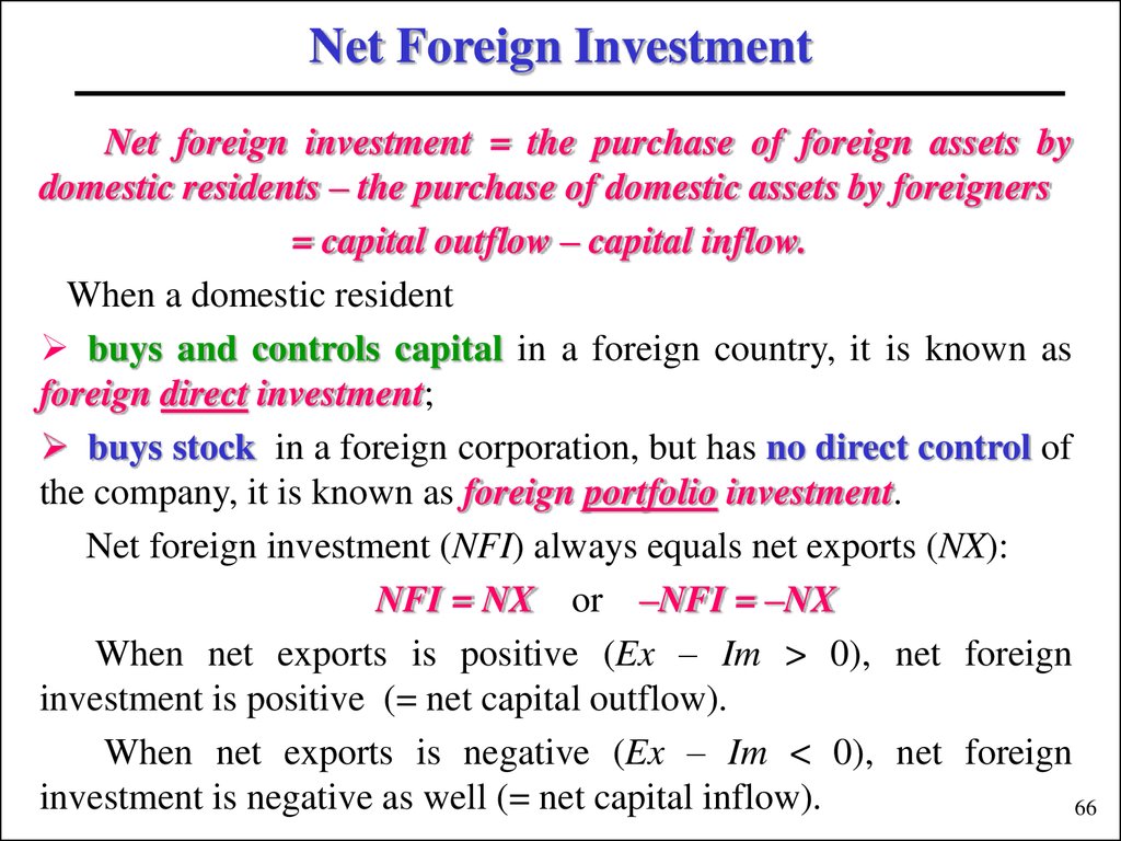
66.
Net Foreign InvestmentNet foreign investment = the purchase of foreign assets by
domestic residents – the purchase of domestic assets by foreigners
= capital outflow – capital inflow.
When a domestic resident
buys and controls capital in a foreign country, it is known as
foreign direct investment;
buys stock in a foreign corporation, but has no direct control of
the company, it is known as foreign portfolio investment.
Net foreign investment (NFI) always equals net exports (NX):
NFI = NX or –NFI = –NX
When net exports is positive (Ex – Im > 0), net foreign
investment is positive (= net capital outflow).
When net exports is negative (Ex – Im < 0), net foreign
investment is negative as well (= net capital inflow).
66
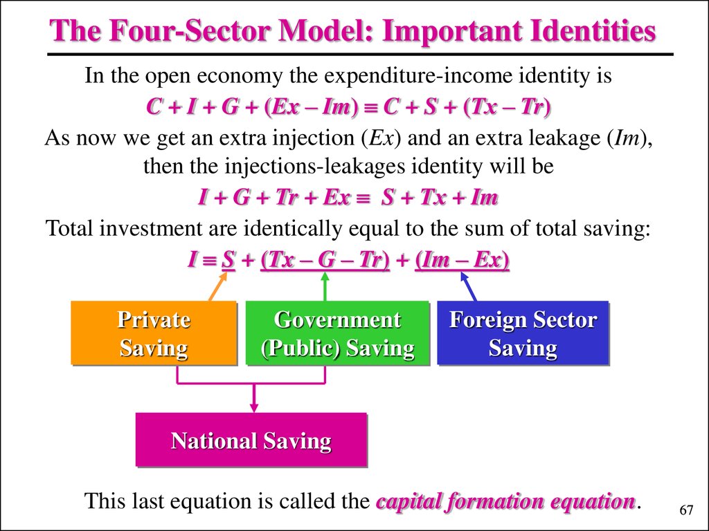
67.
The Four-Sector Model: Important IdentitiesIn the open economy the expenditure-income identity is
C + I + G + (Ex – Im) C + S + (Tх – Tr)
As now we get an extra injection (Ex) and an extra leakage (Im),
then the injections-leakages identity will be
I + G + Tr + Ex S + Tх + Im
Total investment are identically equal to the sum of total saving:
I S + (Tx – G – Tr) + (Im – Ex)
Private
Saving
Government
(Public) Saving
Foreign Sector
Saving
National Saving
This last equation is called the capital formation equation.
67
68.
The Four-Sector Model: Important IdentitiesFrom the injections-leakages identity we can also get
uses-of-private-saving identity:
S I + (G + Tr – Tx) + (Ex – Im)
Financing of
Domestic Investment
Financing of
Budget Deficit
Loan to the
Foreign Sector
budget deficit financing identity:
(G + Tr – Tx) S – (I + NX)
Government
Budget Deficit
Private Sector Fall in Domestic
Saving
Investment
Loan from the
Foreign Sector
68
69. Stock and Flow Variables
Macroeconomic variables can be divided into stocks and flows.A flow is an economic magnitude
measured per a given period of
time (a year, a week, an hour).
All the variables in the model of
circular flows (output, income,
consumption, saving, investment,
taxes, budget deficit, trade
surplus and others) are flows.
A stock is an economic
magnitude measured at a
particular point of time (on
November 1st , 2015).
Examples: wealth, savings,
government
debt, capital
stock, money supply, number
of unemployed, etc.
Flows add to or diminish stocks.
For example, the flow of investment changes the stock of capital;
the flow of budget deficit increases the stock of government debt;
the flow of saving affects the stock of wealth.
69
70.
Stocks and FlowsFLOW
STOCK
STOCK
70
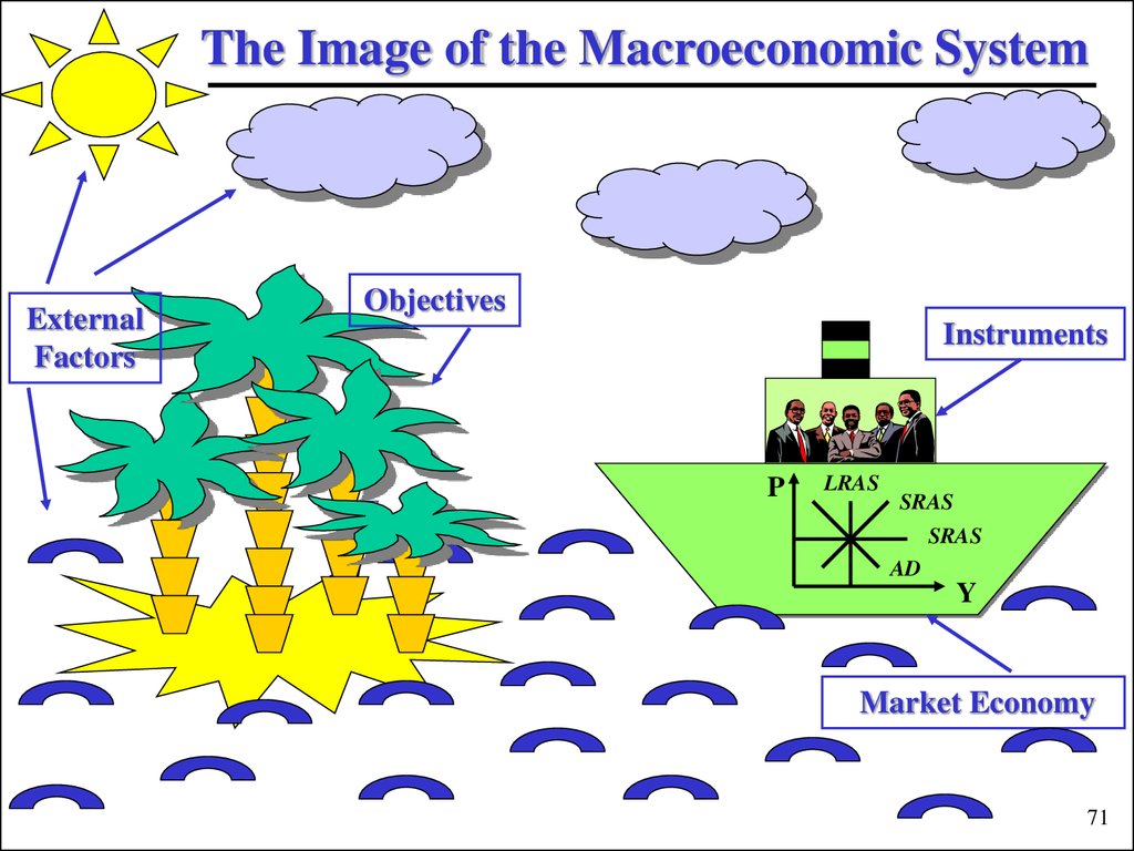
71.
The Image of the Macroeconomic SystemExternal
Factors
Objectives
Instruments
P
LRAS
SRAS
SRAS
AD
Y
Market Economy
71
72. The Macroeconomic System
It is a market economy whichis influenced by
external
(exogenous) factors:
natural (weather,
earthquakes, spots
on the sun, tsunami,
eruptions, etc);
social (revolutions,
wars, overturns, etc)
has objectives
(induced variables):
economic growth;
high employment;
stable prices;
balance of payments
equilibrium.
use instruments
(policy variables):
fiscal policy;
monetary policy;
income policy;
foreign trade and
exchange rate
policy.
Macroeconomic Policy
72
73. Macroeconomic Policy
Economic Growth PolicyStabilization Policy
• is aimed to stimulate economic • is aimed to smooth out business
cycle in the short run and to
growth in the long run and to
diminish the depth of recessions
affect productive possibilities
and the height of booms;
of the economy;
• suggests changes primarily
• suggests changes primarily
in aggregate demand.
in aggregate supply.
73
74. Aggregate Demand and Aggregate Supply
Market Economy: the Key ConceptsAggregate Demand and Aggregate Supply
P
P
LRAS SRAS
Consumption
SRAS
AD
Y
Investment
Government
Spending
Net Exports
Aggregate
Demand
Y*
Y
Aggregate
Supply
Cost of Human
Resources
Cost of Capital
Resources
Cost of Natural
Resources
Equilibrium
Aggregate
Output
Equilibrium
General Price
Level
Technology
74