Similar presentations:
Macroeconomics. Introduction
1. Macroeconomics
Prof. Grigori Feygin2. Introduction
Structure of courseChapter 1 The date and methods of
macroeconomics
Chapter 2-4 The National Accounting
system (not included)
3. Introduction
Structure of courseChapter 5 The Determination of
Output, Income, Expenditure and a
Model of Real Equilibrium
Chapter 6 Money, Prices and the
Interest Rate
4. Introduction
Structure of courseChapter 7 Labour Market,
Employment, Unemployment
Chapter 8 Economic Fluctuations
5. Introduction
Structure of courseChapter 9 The Keynsian Model of
Short-Run Equilibrium
Chapter 10 Aggregate Supply
6. Introduction
Definition“Macroeconomics was born as distinct
in the 1940, as part of intellectual
response to the Great Depression.
The term then referred to the body
of knowledge and expertise that we
hoped would prevent recurrence of
that economic disaster..”
(R. Lucas)
7. Introduction
DefinitionSince then, economic science is
divided into two fields
Microeconomics, which develops
the theories of individual behaviors:
theories of producer, consumer, etc.
8. Introduction
DefinitionSince then, economic science is divided
into two fields
Macroeconomics, which develops the
theories of collective behaviors
The main goal of macroeconomics is to
explain and predict the evolution of
different economic variables, such as
output, employment, money supply,
interest rates, prices, exchange rates,
external
balance,
public
budget
deficit, public debt
9. Introduction
Relationships between two subdisciplinesExamples
- how agents see the future and build
their expectations (micro) can influence
the level of overall consumption (macro)
- the level of public deficit (macro) can get
people to change their saving behaviours
(micro)
10. Introduction
An overview of the macroeconomictheories
Two main theories:
- Classical theory gives a central
place to the notion of equilibrium
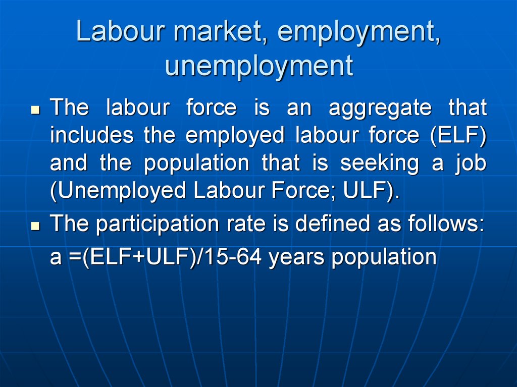
- Keynesian theory – “ sticky
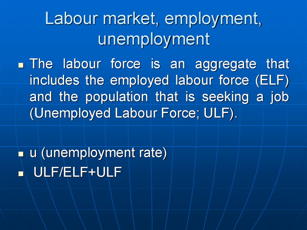
prices macroeconomics”
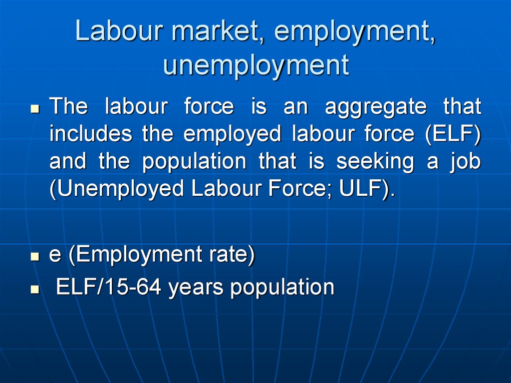
11. Introduction
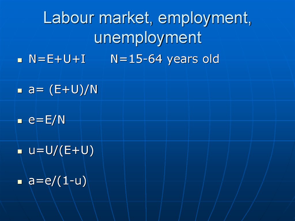
An overview of the macroeconomictheories
Classical theory- economic policies
are not helpful. Market can be
cleared in the short run without the
necessity of external intervention.
12. Introduction
An overview of the macroeconomictheories
Keynesian theory – economic policies
are useful because the return to
equilibrium for the economy is
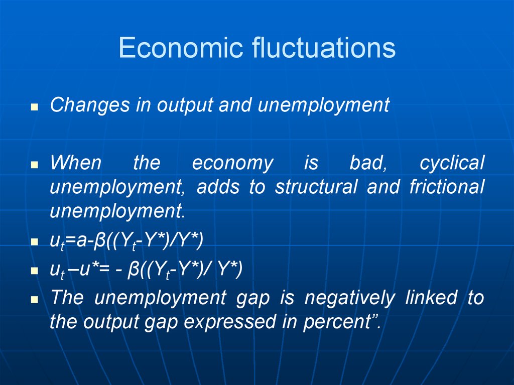
neither automatic nor immediate.
13. Introduction
An overview of the macroeconomictheories
Classical theoryHypothesis of flexible prices,
macroeconomic theories may be
useful to explain the functioning
of the economy in the long run.
14. Introduction
An overview of the macroeconomictheories
Keynsian theory helps to explain
the short-run fluctuations in the
level of activity that generate
disequilibrium.
15. Introduction
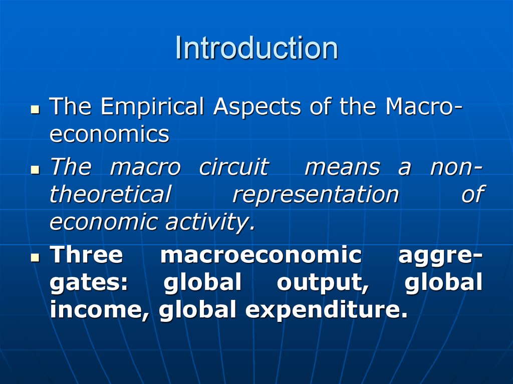
The Empirical Aspects of the MacroeconomicsThe macro circuit
means a nontheoretical
representation
of
economic activity.
Three
macroeconomic
aggregates: global output, global
income, global expenditure.
16. Introduction
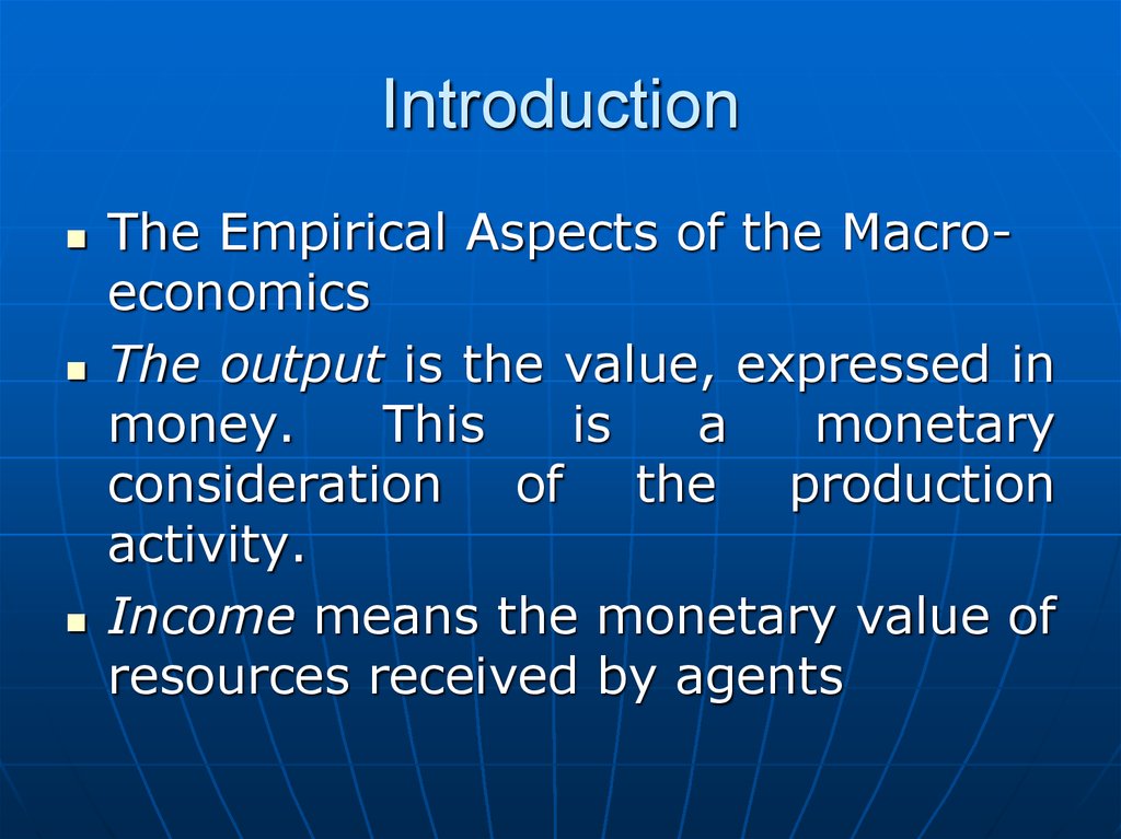
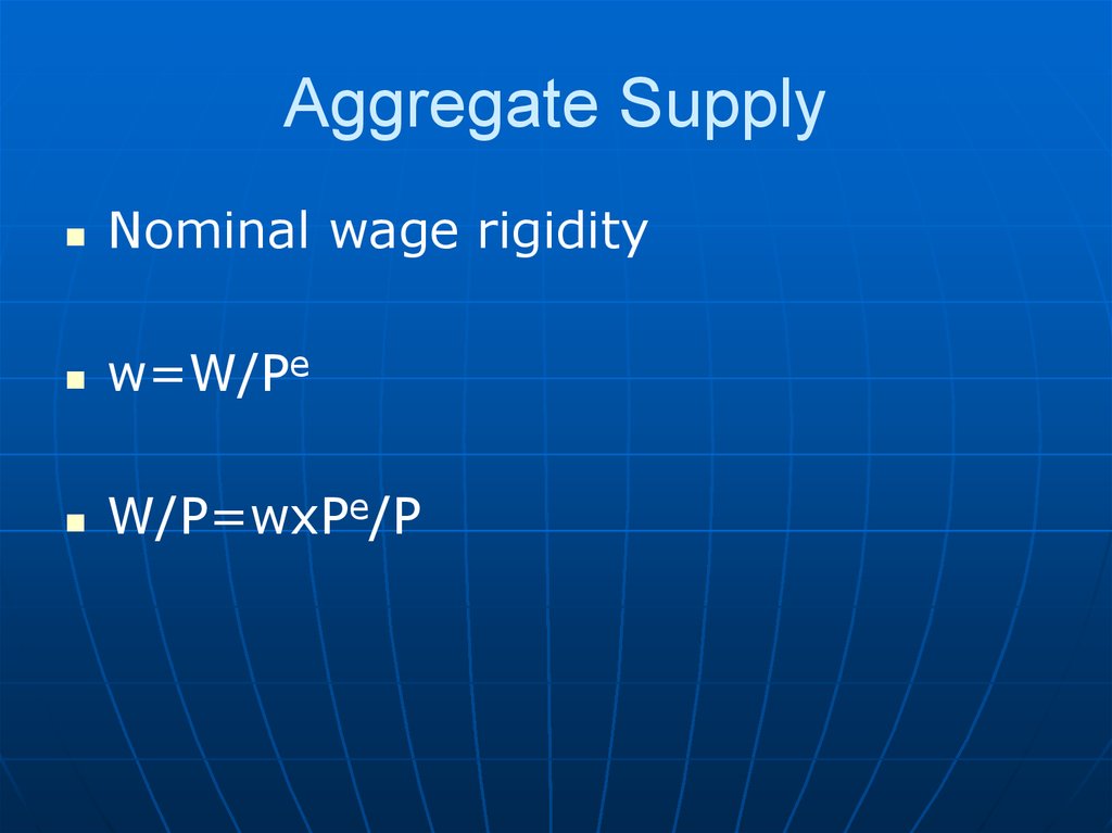
The Empirical Aspects of the MacroeconomicsThe output is the value, expressed in
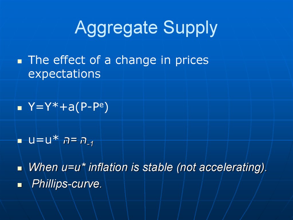
money.
This
is
a
monetary
consideration of the production
activity.
Income means the monetary value of
resources received by agents
17. Introduction
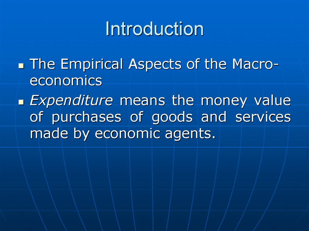
The Empirical Aspects of the MacroeconomicsExpenditure means the money value
of purchases of goods and services
made by economic agents.
18. Introduction
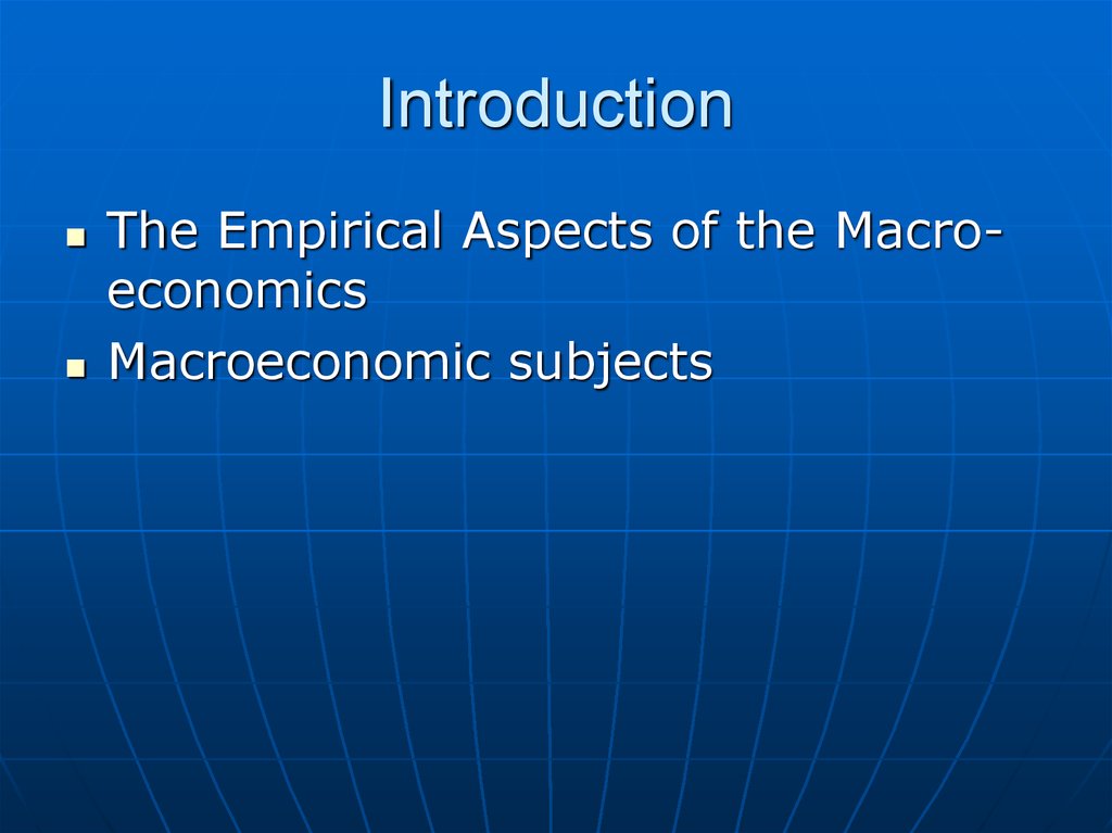
The Empirical Aspects of the MacroeconomicsMacroeconomic subjects
19. Introduction
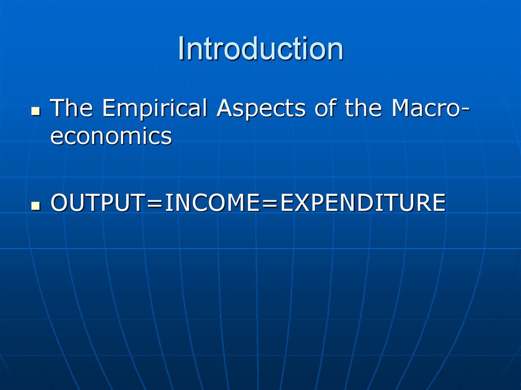
The Empirical Aspects of the MacroeconomicsOUTPUT=INCOME=EXPENDITURE
20. Introduction
The measurement of macroeconomicfacts
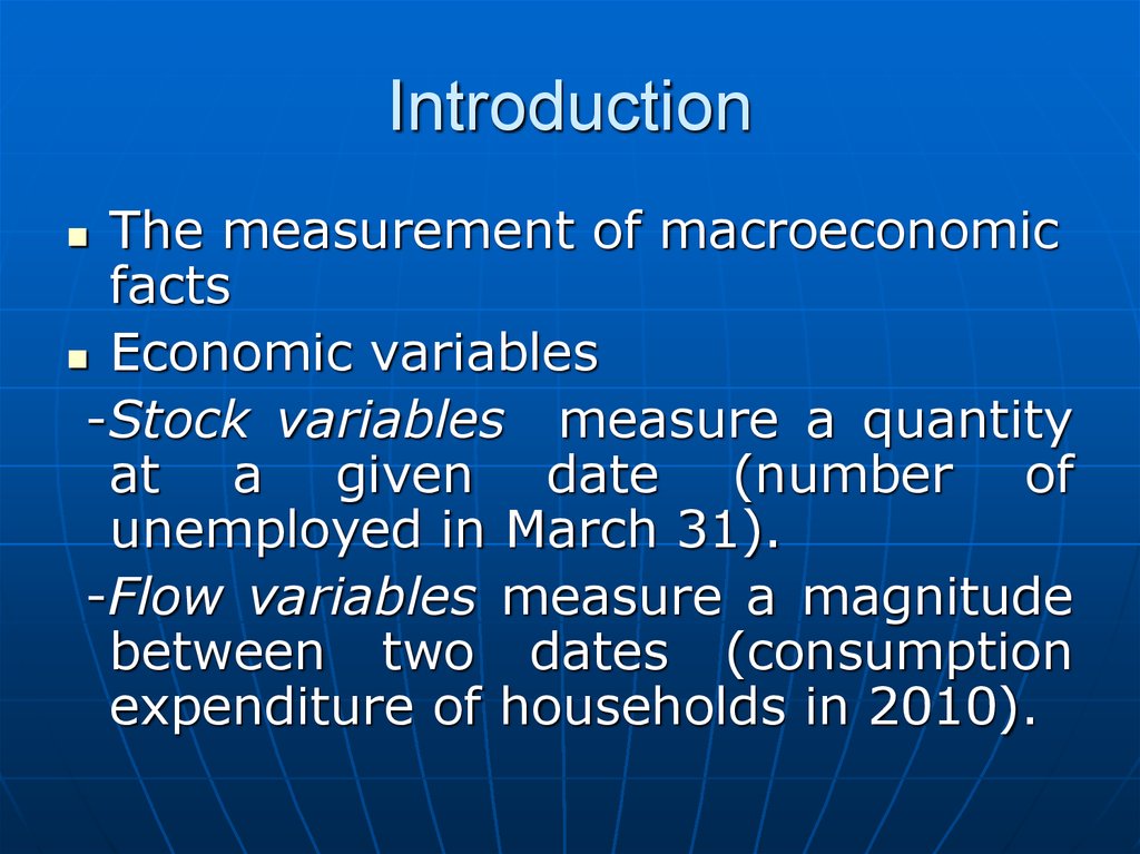
Economic variables
-Stock variables measure a quantity
at a given date (number of
unemployed in March 31).
-Flow variables measure a magnitude
between two dates (consumption
expenditure of households in 2010).
21. Introduction
-The measurement of macroeconomic
facts
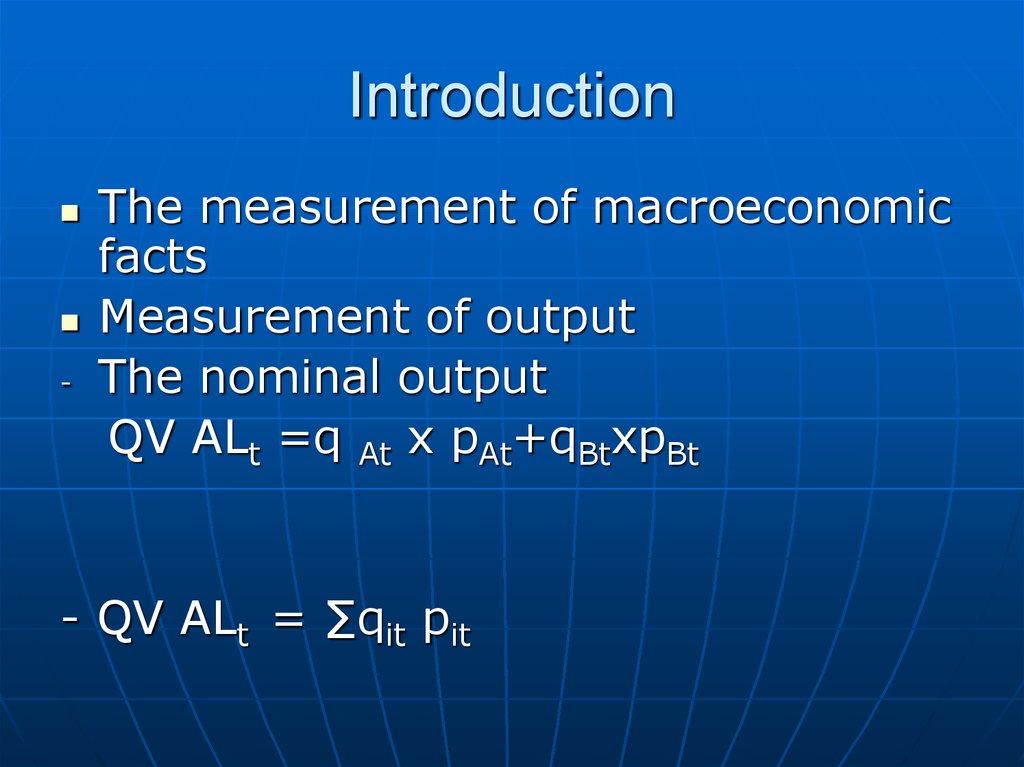
Measurement of output
The nominal output
QV ALt =q At x pAt+qBtxpBt
- QV ALt = ∑qit pit
22. Introduction
-The measurement of macroeconomic
facts
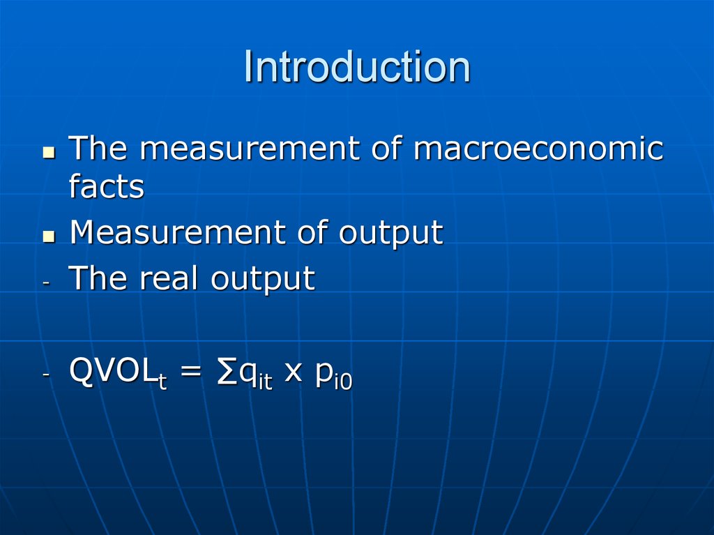
Measurement of output
The real output
-
QVOLt = ∑qit x pi0
23. Introduction
-The measurement of macroeconomic facts
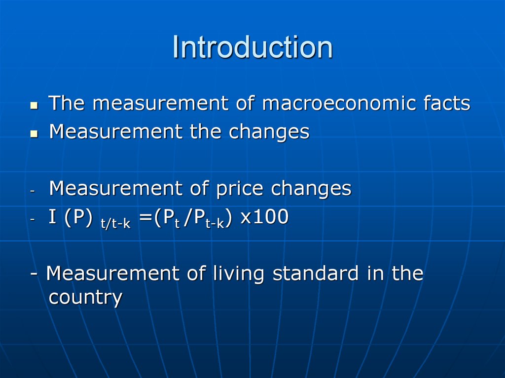
Measurement the changes
Measurement of price changes
I (P) t/t-k =(Pt /Pt-k) x100
- Measurement of living standard in the
country
24. Introduction
The measurement of macroeconomicfacts
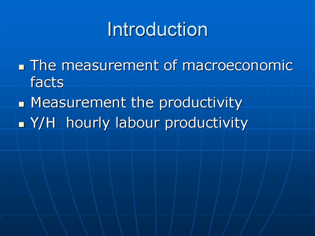
Measurement the productivity
Y/H hourly labour productivity
25. Introduction
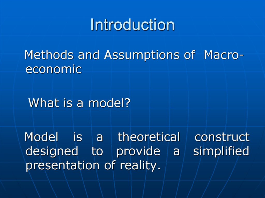
Methods and Assumptions of MacroeconomicWhat is a model?
Model is a theoretical
designed to provide a
presentation of reality.
construct
simplified
26. Introduction
Methods and Assumptions of MacroeconomicWhat is a model?
Example- a
equilibrium
model
of
economic
27. The determination of Output, Income, Expenditure and a model of Real Equilibrium
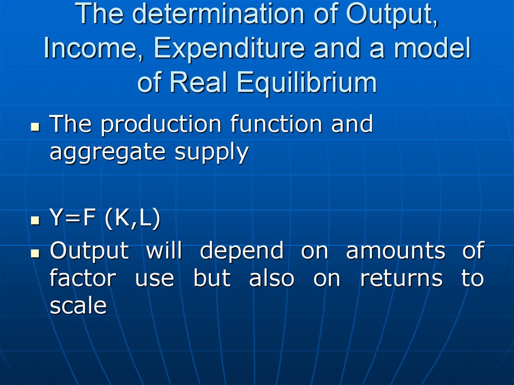
The production function andaggregate supply
Y=F (K,L)
Output will depend on amounts of
factor use but also on returns to
scale
28. The determination of Output, Income, Expenditure and a model of Real Equilibrium
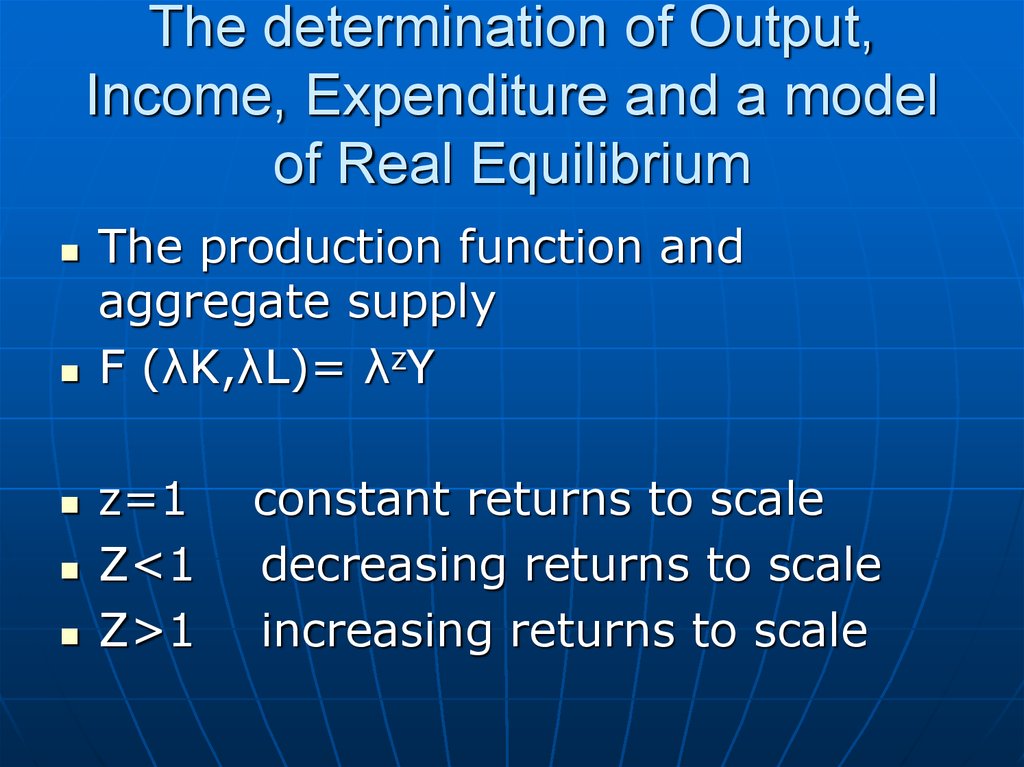
The production function andaggregate supply
F (λK,λL)= λzY
z=1
Z<1
Z>1
constant returns to scale
decreasing returns to scale
increasing returns to scale
29. The determination of Output, Income, Expenditure and a model of Real Equilibrium
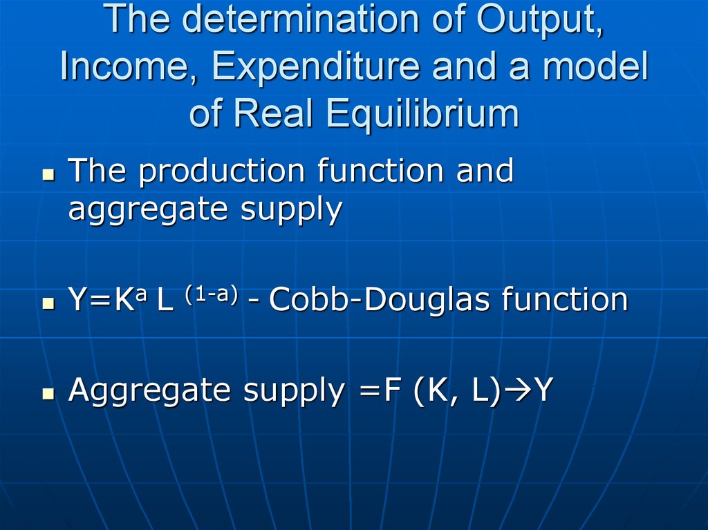
The production function andaggregate supply
Y=Ka L
Aggregate supply =F (K, L) Y
(1-a)
- Cobb-Douglas function
30. The determination of Output, Income, Expenditure and a model of Real Equilibrium
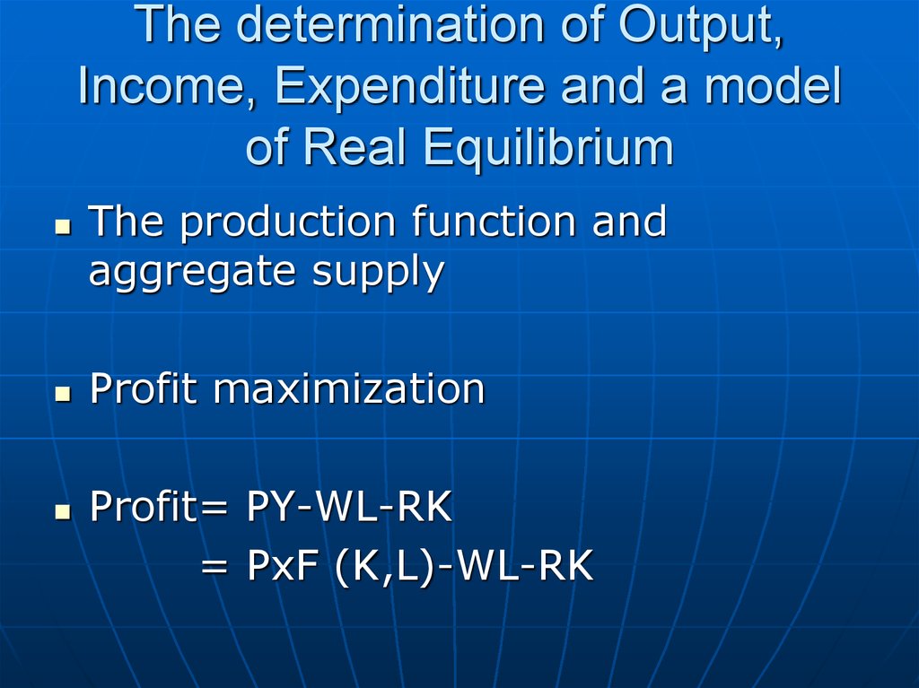
The production function andaggregate supply
Profit maximization
Profit= PY-WL-RK
= PxF (K,L)-WL-RK
31. The determination of Output, Income, Expenditure and a model of Real Equilibrium
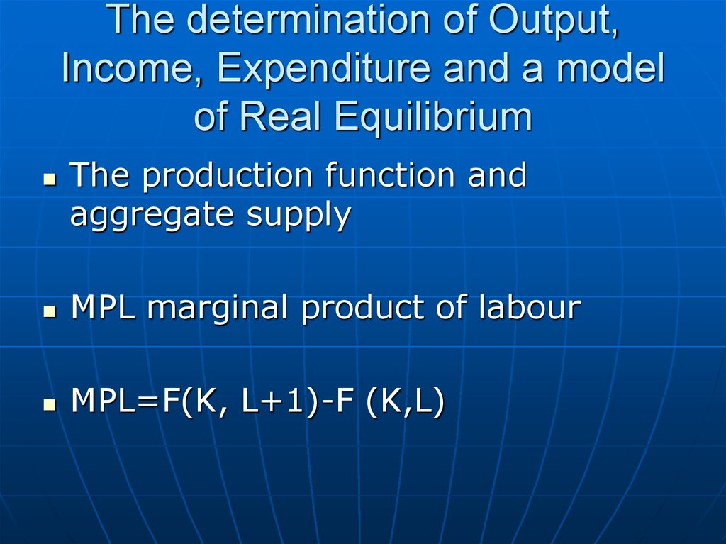
The production function andaggregate supply
MPL marginal product of labour
MPL=F(K, L+1)-F (K,L)
32. The determination of Output, Income, Expenditure and a model of Real Equilibrium
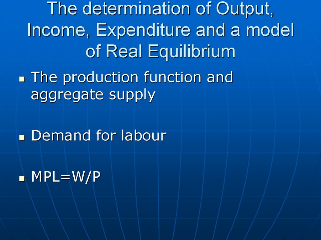
The production function andaggregate supply
Demand for labour
MPL=W/P
33. The determination of Output, Income, Expenditure and a model of Real Equilibrium
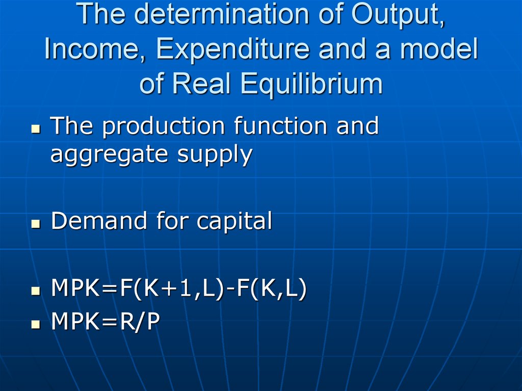
The production function andaggregate supply
Demand for capital
MPK=F(K+1,L)-F(K,L)
MPK=R/P
34. The determination of Output, Income, Expenditure and a model of Real Equilibrium
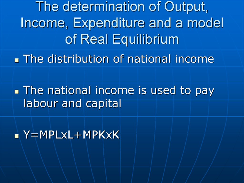
The distribution of national incomeThe national income is used to pay
labour and capital
Y=MPLxL+MPKxK
35. The determination of Output, Income, Expenditure and a model of Real Equilibrium
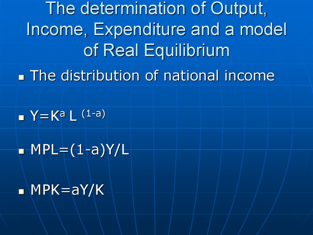
The distribution of national incomeY=Ka L
MPL=(1-a)Y/L
MPK=aY/K
(1-a)
36. The determination of Output, Income, Expenditure and a model of Real Equilibrium
The distribution of national incomeY=Ka L
MPL=(1-a)Y/L
MPK=aY/K
(1-a)
37. The determination of Output, Income, Expenditure and a model of Real Equilibrium
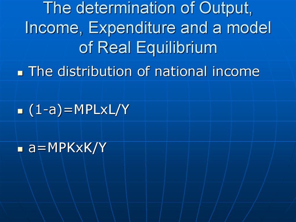
The distribution of national income(1-a)=MPLxL/Y
a=MPKxK/Y
38. The determination of Output, Income, Expenditure and a model of Real Equilibrium
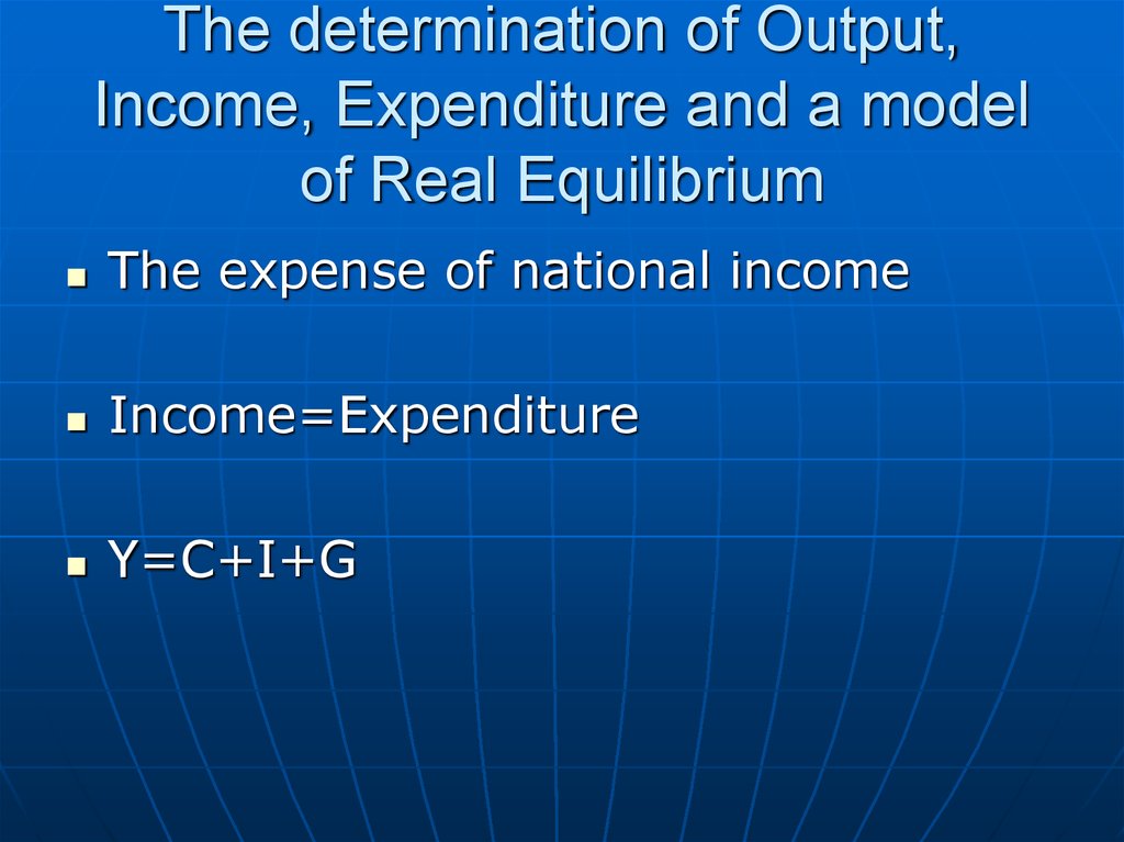
The expense of national incomeIncome=Expenditure
Y=C+I+G
39. The determination of Output, Income, Expenditure and a model of Real Equilibrium
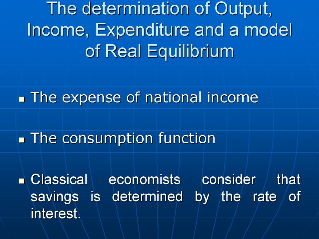
The expense of national incomeThe consumption function
Classical economists consider that
savings is determined by the rate of
interest.
40. The determination of Output, Income, Expenditure and a model of Real Equilibrium
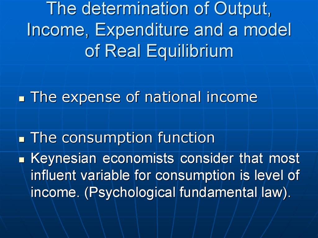
The expense of national incomeThe consumption function
Keynesian economists consider that most
influent variable for consumption is level of
income. (Psychological fundamental law).
41. The determination of Output, Income, Expenditure and a model of Real Equilibrium
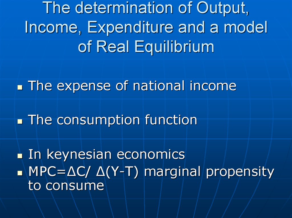
The expense of national incomeThe consumption function
In keynesian economics
MPC=∆C/ ∆(Y-T) marginal propensity
to consume
42. The determination of Output, Income, Expenditure and a model of Real Equilibrium
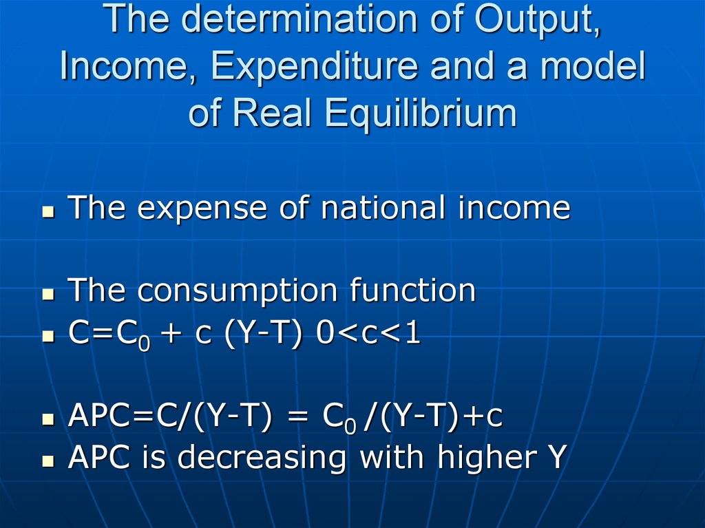
The expense of national incomeThe consumption function
C=C0 + c (Y-T) 0<c<1
APC=C/(Y-T) = C0 /(Y-T)+c
APC is decreasing with higher Y
43. The determination of Output, Income, Expenditure and a model of Real Equilibrium
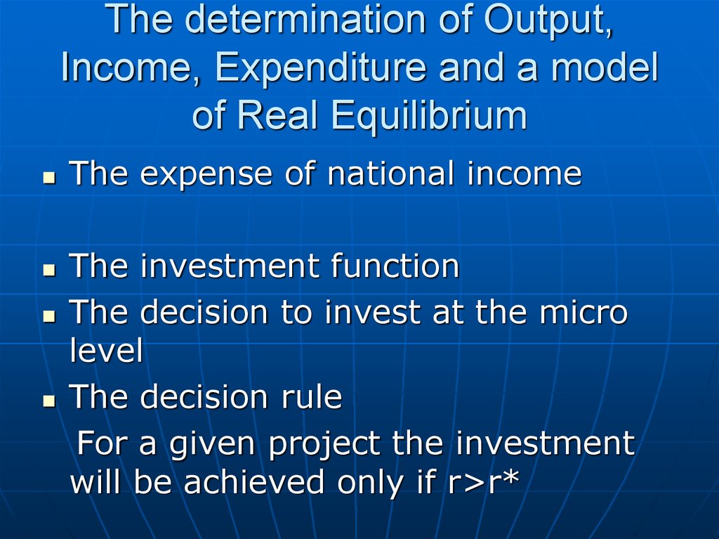
The expense of national incomeThe investment function
The decision to invest at the micro
level
The decision rule
For a given project the investment
will be achieved only if r>r*
44. The determination of Output, Income, Expenditure and a model of Real Equilibrium
The expense of national incomeThe investment function
The decision to invest at the macro
level
Selection of investment projects with
r>r*
45. The determination of Output, Income, Expenditure and a model of Real Equilibrium
The expense of national incomePublic spending
- operating expenses
- capital expenses
- expenditure of social security
- debt service
46. The determination of Output, Income, Expenditure and a model of Real Equilibrium
The expense of national incomePublic spending
The
government
must
fund
these
expenses. Expenditures must be offset by
equivalent receipts obtained
- by taxes
- borrowing through net issuance of debt
securities
- printing money
47. The determination of Output, Income, Expenditure and a model of Real Equilibrium
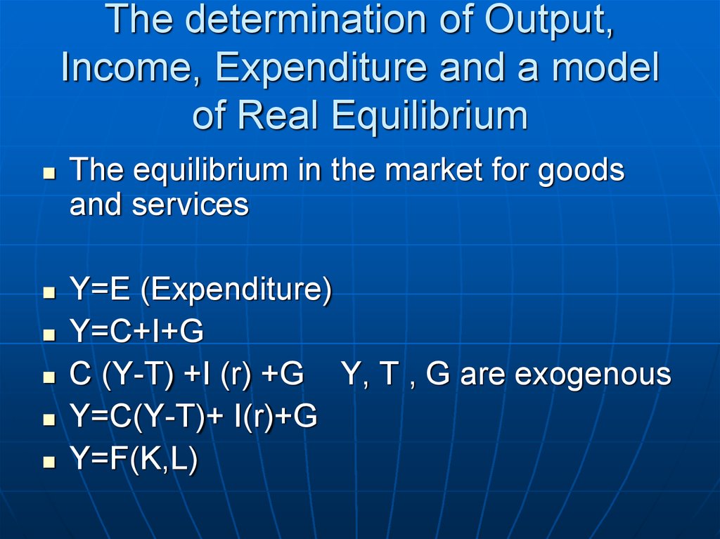
The equilibrium in the market for goodsand services
Y=E (Expenditure)
Y=C+I+G
C (Y-T) +I (r) +G Y, T , G are exogenous
Y=C(Y-T)+ I(r)+G
Y=F(K,L)
48. The determination of Output, Income, Expenditure and a model of Real Equilibrium
The equilibrium in the financial market: the roleof the interest rate
A) Savings
S=Y-C-G
S=(Y-T-G) +(T-G)
(Y-T-C)- private savings
(T-G) –public savings
49. The determination of Output, Income, Expenditure and a model of Real Equilibrium
The equilibrium in the financial market: the roleof the interest rate
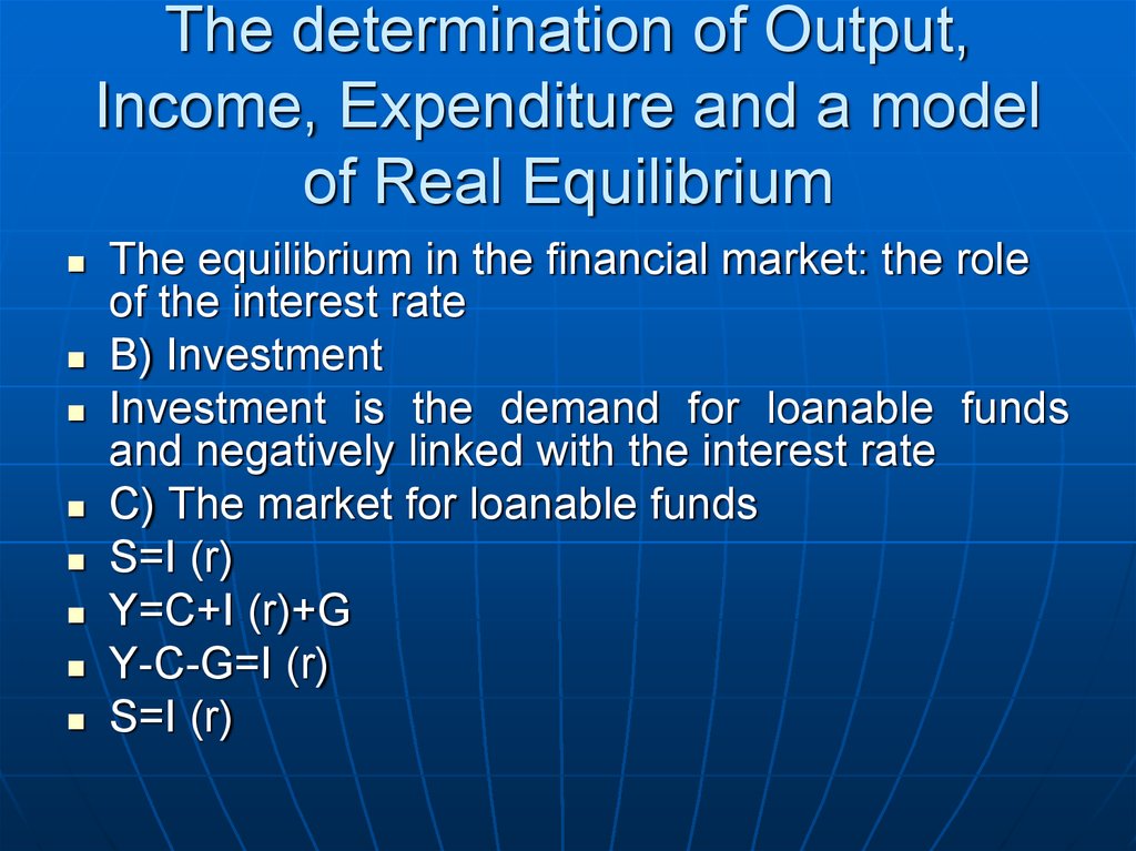
B) Investment
Investment is the demand for loanable funds
and negatively linked with the interest rate
C) The market for loanable funds
S=I (r)
Y=C+I (r)+G
Y-C-G=I (r)
S=I (r)
50. The determination of Output, Income, Expenditure and a model of Real Equilibrium
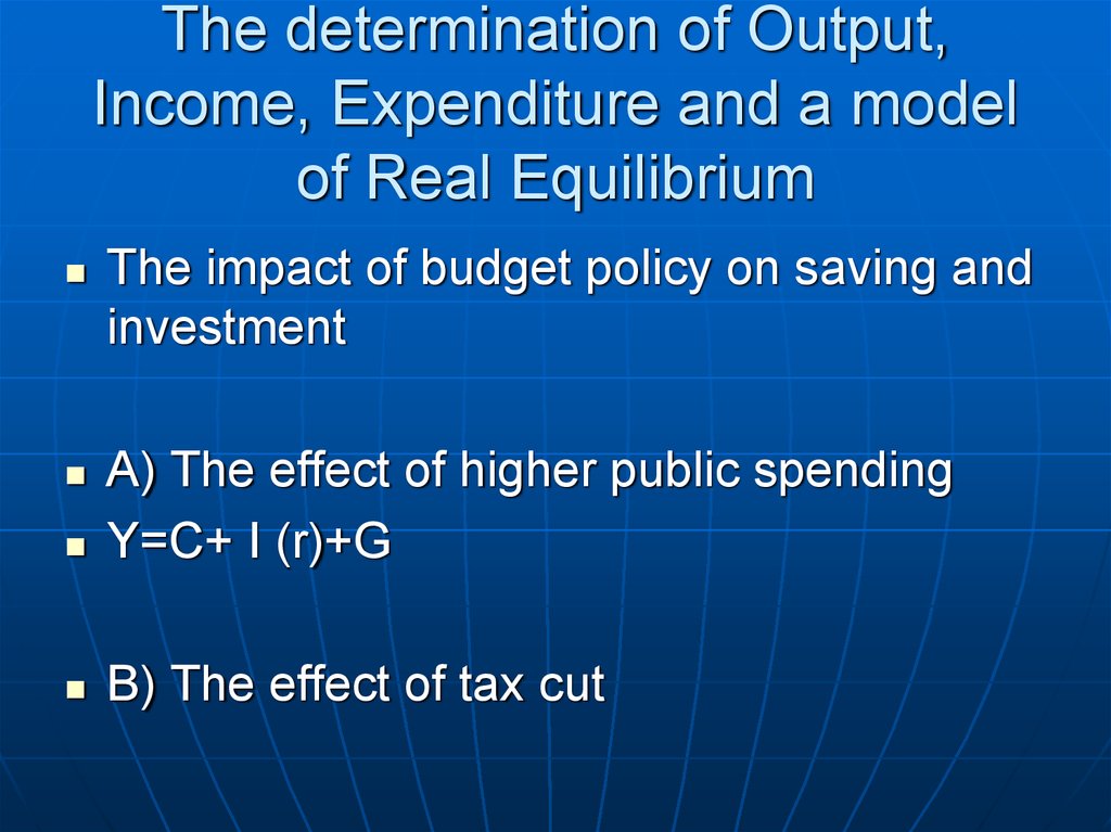
The impact of budget policy on saving andinvestment
A) The effect of higher public spending
Y=C+ I (r)+G
B) The effect of tax cut
51. Money, prices and interest rates
What is the impact of change in thequantity of money on the functioning of
economy
What connection is there between the
interest rate, demand for money and price
trends
What problems between too large
fluctuations in the price level.
52. Money, prices and interest rates
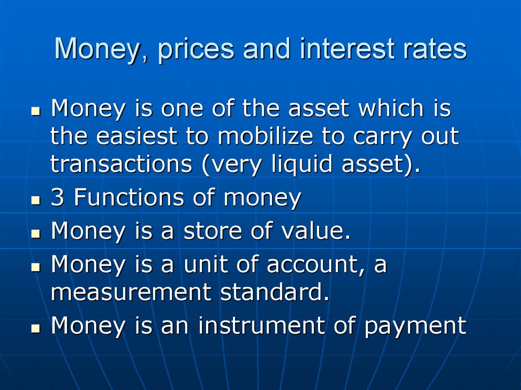
Money is one of the asset which isthe easiest to mobilize to carry out
transactions (very liquid asset).
3 Functions of money
Money is a store of value.
Money is a unit of account, a
measurement standard.
Money is an instrument of payment
53. Money, prices and interest rates
Agents will want to have a greater orlesser amount of these asset as
needed. So there is a demand for
money, as well as for any good or
asset.
The money supply is controlled the
banking system, consisting of regular
banks under the authority of central
bank.
54. Money, prices and interest rates
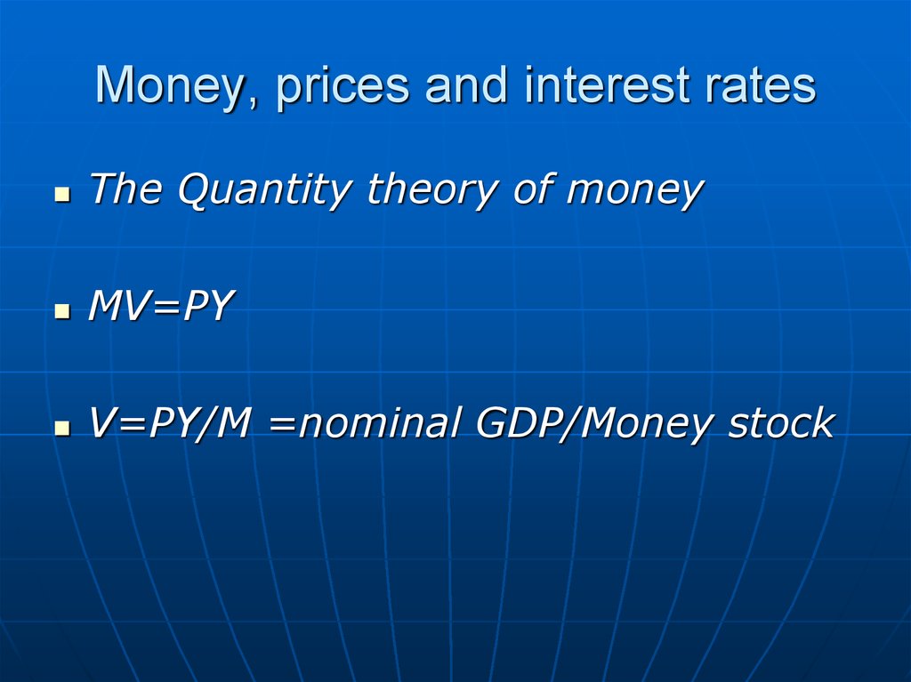
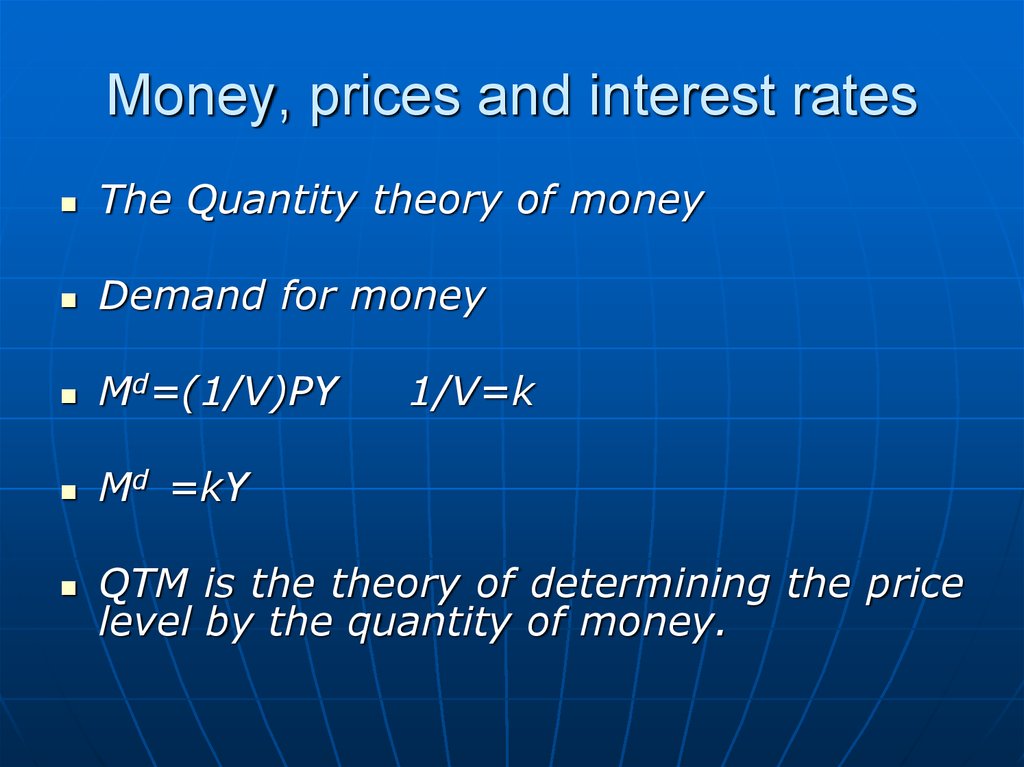
The Quantity theory of moneyMV=PY
V=PY/M =nominal GDP/Money stock
55. Money, prices and interest rates
The Quantity theory of moneyDemand for money
Md=(1/V)PY
Md =kY
QTM is the theory of determining the price
level by the quantity of money.
1/V=k
56. Money, prices and interest Rates
The Interest Rate, the demand for moneyand Inflation
The nominal interest rate (NIR) is the rate
of change of an amount of money during a
period when the is the subject of a loan.
The real interest rate (RIR) is the rate of
variation in the purchasing power of
money.
57. Money, prices and interest Rates
The Interest Rate, the demand for moneyand Inflation
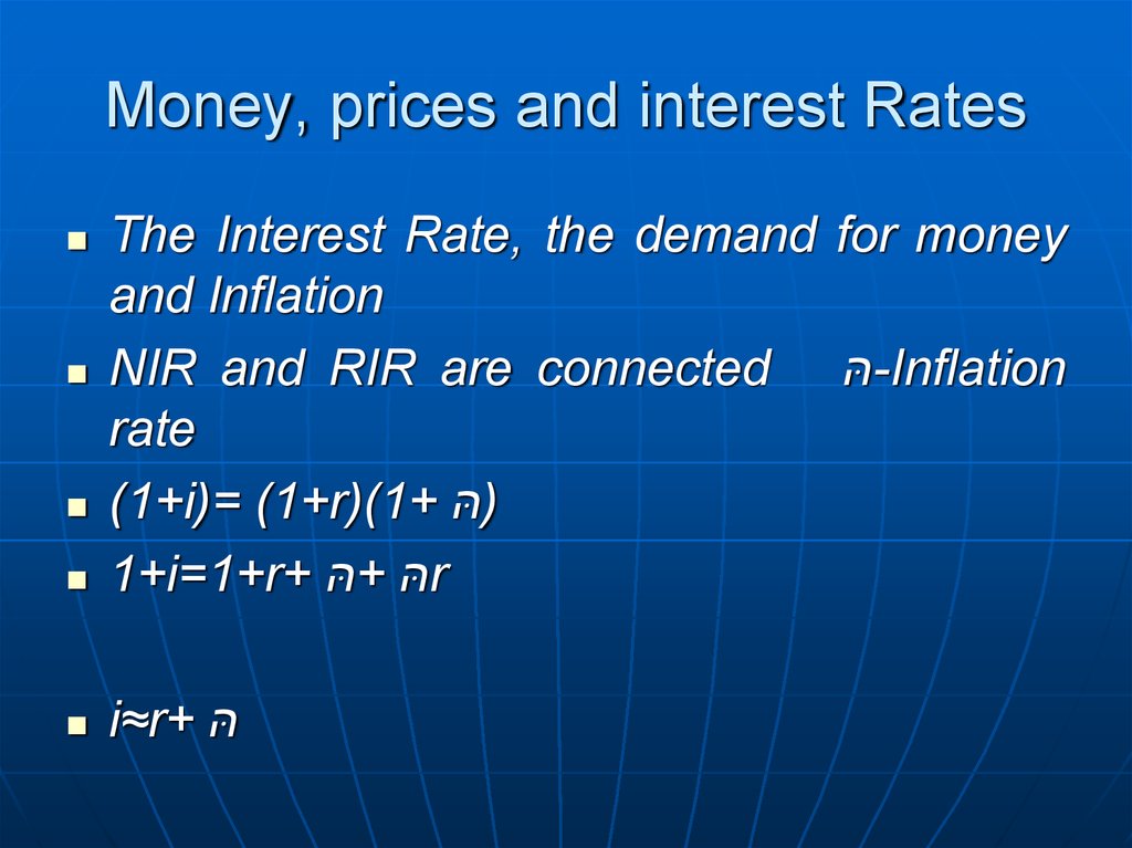
NIR and RIR are connected -Inflation
rate
(1+i)= (1+r)(1+ )
1+i=1+r+ + r
i≈r+
58. Money, prices and interest Rates
The Interest Rate, the demand for moneyand Inflation
NIR depends on:
-the real interest rate, itself determined
between savings and investment
- expected inflation
i=r+ e
59. Money, prices and interest Rates
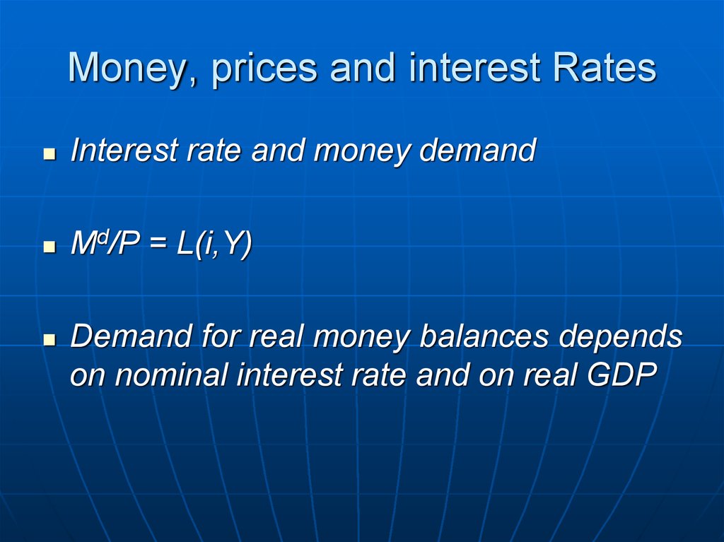
Interest rate and money demandMd/P = L(i,Y)
Demand for real money balances depends
on nominal interest rate and on real GDP
60. Money, prices and interest Rates
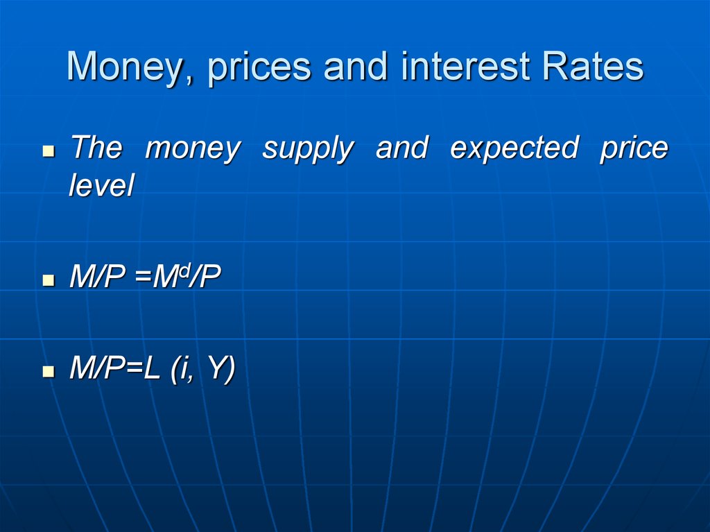
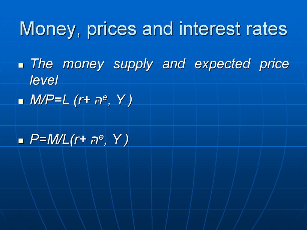
The money supply and expected pricelevel
M/P =Md/P
M/P=L (i, Y)
61. Money, prices and interest rates
The money supply and expected pricelevel
M/P=L (r+ e, Y )
P=M/L(r+ e, Y )
62. Money, prices and interest rates
The Problems with Too Large Fluctuationin Price Level
Inflation is a general rise in prices of goods
and services.
Its effects on money functions
Inflation creates many distortions
63. Money, prices and interest rates
The Problems with Too Large Fluctuationin Price Level
Deflation is the symmetrical situation of
inflation.
64. Labour market, employment, unemployment
Labour demand comes from companies that want to produce.Labour supply comes from individuals who wish to earn an income.
65. Labour market, employment, unemployment
The labour force is an aggregate thatincludes the employed labour force (ELF)
and the population that is seeking a job
(Unemployed Labour Force; ULF).
The participation rate is defined as follows:
a =(ELF+ULF)/15-64 years population
66. Labour market, employment, unemployment
The labour force is an aggregate thatincludes the employed labour force (ELF)
and the population that is seeking a job
(Unemployed Labour Force; ULF).
u (unemployment rate)
ULF/ELF+ULF
67. Labour market, employment, unemployment
The labour force is an aggregate thatincludes the employed labour force (ELF)
and the population that is seeking a job
(Unemployed Labour Force; ULF).
e (Employment rate)
ELF/15-64 years population
68. Labour market, employment, unemployment
N=E+U+Ia= (E+U)/N
e=E/N
u=U/(E+U)
a=e/(1-u)
N=15-64 years old
69. Labour market, employment, unemployment
Share of long length unemployed(those unemployed for one year and
more) in the total unemployed.
Average duration of unemployment
70. Labour market, employment, unemployment
The flow of workersIt is the number of people who, over
time, get in and out of employment
status.
Flow of jobs
Net job flow=flow of job creationflow of job destruction
71. The Long-Run Rate of Unemployment
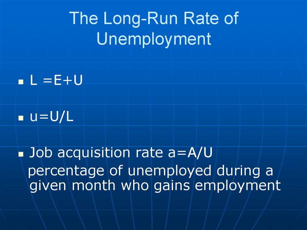
L =E+Uu=U/L
Job acquisition rate a=A/U
percentage of unemployed during a
given month who gains employment
72. The Long-Run Rate of Unemployment
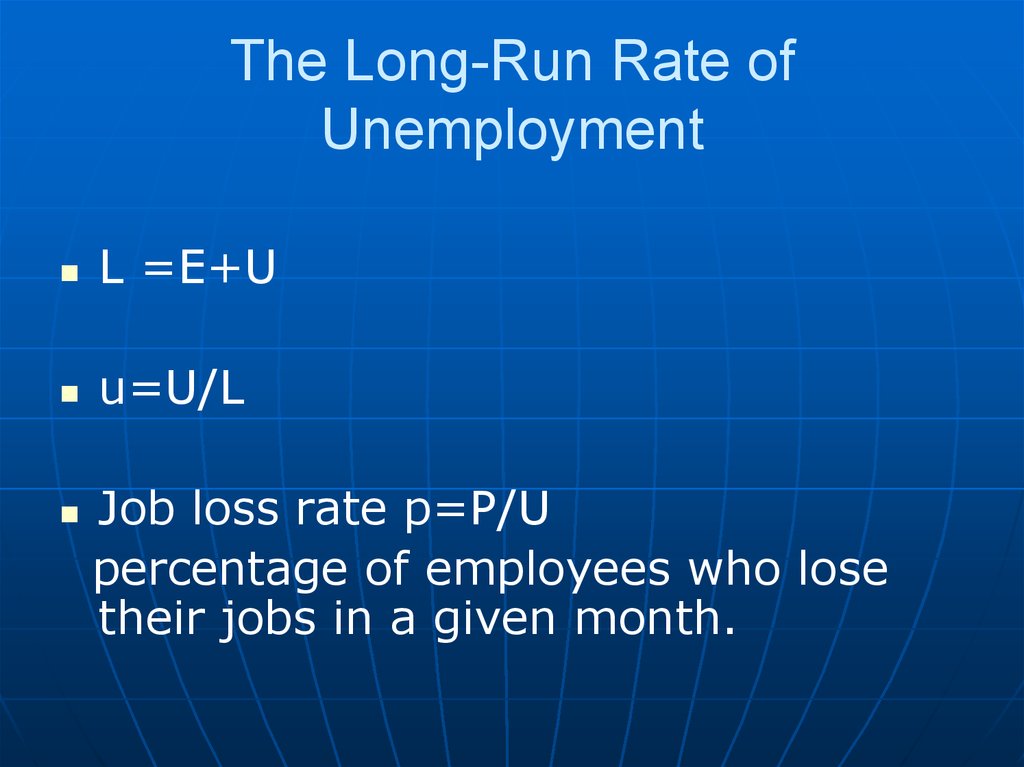
L =E+Uu=U/L
Job loss rate p=P/U
percentage of employees who lose
their jobs in a given month.
73. The Long-Run Rate of Unemployment
Natural rate of unemployment=longrun rate of unemploymentA=P
74. Economic fluctuations
Theeconomy
is
experiencing
fluctuations that result in variations
in the level of output around its longrun trend. The existence of these
fluctuations leads to talk about
business cycle.
75. Economic fluctuations
Accelerationboom)
phases
(economic
Contraction
recession)
phase
(economic
76. Economic fluctuations
Changes in output and unemploymentWhen the economy is bad, cyclical
unemployment, adds to structural and
frictional unemployment.
The relationship between output level and
unemployment is known as “Okun,s law”
77. Economic fluctuations
Changes in output and unemploymentWhen the economy is bad, cyclical
unemployment, adds to structural and
frictional unemployment.
Okun consider that: the unemployment
rate is negatively linked to the level of
output.
78. Economic fluctuations
Changes in output and unemploymentWhen
the
economy
is
bad,
cyclical
unemployment, adds to structural and frictional
unemployment.
ut=a-β((Yt-Y*)/Y*)
ut –u*= - β((Yt-Y*)/ Y*)
The unemployment gap is negatively linked to
the output gap expressed in percent”.
79. Economic fluctuations
Aggregate demand and aggregate supplyThe aggregate demand is deduced from
the quantity aquation of money.
The AD curve is the curve reflecting, at the
macroeconomic level, the relationship
between the demanded quontities of
goods and price level (for a given level of
money supply and velocity).
80. Economic fluctuations
Aggregate demand and aggregate supplyThe aggregate supply
The long-run aggregate supply (LRAS)
Production function Y=f (K,L)
The short-run aggregate supply (SRAS)
Rigidity of prices
81. Economic fluctuations
Aggregate demand and aggregate supplyAS-AD model
Long-run effect of change in AD
In the long run only the price level is
effected.
82. Economic fluctuations
Aggregate demand and aggregate supplyAS-AD model
Short-run effect of change in AD
In the short run, an AD decrease reduces
the activity level of the economy which can
fall in a recession. Prices are pushed
down. An increase pushes output up and
prices too.
83. Economic fluctuations
--
Aggregate demand and aggregate supply
AS-AD model
The Effect of Monetary Policy
The Central bank can reduce the money supply
The M decrease reduces AD, which affects the
level of output Y and the economy enters a
recession.
Over time, given the weak demand, prices will
decrease. The prices decrease brings the
economy towards its long-run equilibrium.
84. Economic fluctuations
Aggregate demand and aggregate supplyAS-AD model
The Effect of Monetary Policy
1) a decrease in output in the short run, then
a return to the long-run value
2) price stability in the short run and lower
prices over time
85. Economic fluctuations
Aggregate demand and aggregate supplyAS-AD model
The Effect of Monetary Policy
1) a decrease in output in the short run, then
a return to the long-run value
2) price stability in the short run and lower
prices over time
86. Economic fluctuations
Aggregate demand and aggregate supplyAS-AD model
The Effect of Monetary Policy
1) a decrease in output in the short run, then
a return to the long-run value
2) price stability in the short run and lower
prices over time
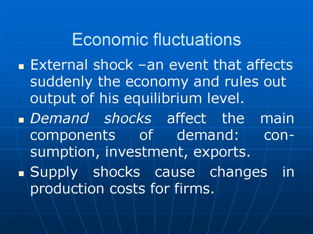
87. Economic fluctuations
External shock –an event that affectssuddenly the economy and rules out
output of his equilibrium level.
Demand shocks affect the main
components
of
demand:
consumption, investment, exports.
Supply shocks cause changes in
production costs for firms.
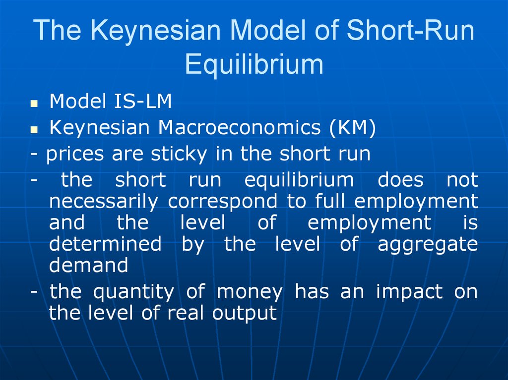
88. The Keynesian Model of Short-Run Equilibrium
Model IS-LMKeynesian Macroeconomics (KM)
- prices are sticky in the short run
- the short run equilibrium does not
necessarily correspond to full employment
and
the
level
of
employment
is
determined by the level of aggregate
demand
- the quantity of money has an impact on
the level of real output
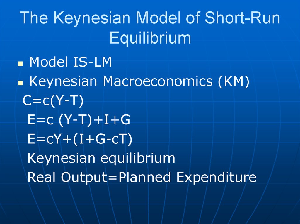
89. The Keynesian Model of Short-Run Equilibrium
Model IS-LMKeynesian Macroeconomics (KM)
C=c(Y-T)
E=c (Y-T)+I+G
E=cY+(I+G-cT)
Keynesian equilibrium
Real Output=Planned Expenditure
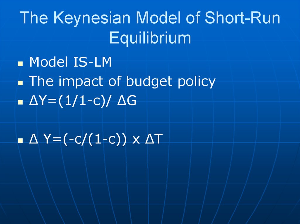
90. The Keynesian Model of Short-Run Equilibrium
Model IS-LMThe impact of budget policy
∆Y=(1/1-c)/ ∆G
∆ Y=(-c/(1-c)) x ∆T
91. The Keynesian Model of Short-Run Equilibrium
Model IS-LMThe impact of budget policy
Balanced budget
∆Y= ∆G ∆
92. The Keynesian Model of Short-Run Equilibrium
Model IS-LMI =I(r)
IS curve shows all possible combinations of income and interest rate
that are consistent with equilibrium
in the market for goods and services.
93. The Keynesian Model of Short-Run Equilibrium
Model IS-LMBudget policy and IS-curve
- An increase in public spending or a
decrease in taxes moves IS to the
right
- Lower public spending or higher
taxes moves IS to the left.
94. The Keynesian Model of Short-Run Equilibrium
Model IS-LMMoney market and LM Curve
The money supply
-the money supply is exogenous and
depends on the central bank;
-prices are fixed in the short run
95. The Keynesian Model of Short-Run Equilibrium
Model IS-LMMoney market and LM Curve
The demand for money
Md/P=L(i,Y)
- transaction motive
- a care motive
- speculative motive
96. The Keynesian Model of Short-Run Equilibrium
Model IS-LMDefinition: the LM curve represents
all possible combinations of interest
rate and income levels that meet the
equilibrium of money market.
97. The Keynesian Model of Short-Run Equilibrium
Model IS-LMShort-Run Equilibrium
Y=C(Y-T)+I(r)+G
M/P=L(i,Y)
98. The Keynesian Model of Short-Run Equilibrium
Model IS-LMEconomic Policy through the IS-LM
model.
The stabilization of the economy
through budget policy
-The case of a rise in public spending
-The case of tax-cut
99. The Keynesian Model of Short-Run Equilibrium
--
Model IS-LM
Economic Policy through the IS-LM
model.
The stabilization of activity by
monetary policy
The interaction of budget and
monetary policies
100. The Keynesian Model of Short-Run Equilibrium
Model IS-LMIS-LM and aggregate demand
IS-LM and deflation
101. Aggregate Supply
LRAS –level of output is determinedonly by amounts of factors available.
SRAS is based on the assumption of
sticky prices in the short run
(Y-Y*)=a(P-Pe)
102. Aggregate Supply
Nominal wage rigidityw=W/Pe
W/P=wxPe/P
103. Aggregate Supply
The effect of a change in pricesexpectations
Y=Y*+a(P-Pe)
u=u* = -1
When u=u* inflation is stable (not accelerating).
Phillips-curve.











 economics


