Aggregate demand and aggregate supply: Figure 13.6

The long-run aggregate supply curve: Figure 13.7

How expectations of the future price level affect the short-run aggregate supply: Figure 13.8

Macroeconomic equilibrium in the long run and the short run

Long-run macroeconomic equilibrium: Figure 13.9

The short-run and long-run effects of a decrease in aggregate demand: Figure 13.10

The short-run and long-run effects of an increase in aggregate demand: Figure 13.11

The short-run and long-run effects of a supply shock: Figure 13.12

A dynamic aggregate demand and aggregate supply model

A dynamic aggregate demand and aggregate supply model: Figure 13.13

Using dynamic aggregate demand and aggregate supply to understand inflation: Figure 13.14

4.99M

Category:

economics

Aggregate demand and aggregate supply analysis

1. Chapter 13

PowerPoint
to accompany
Chapter 13
Aggregate
Demand and
Aggregate
Supply Analysis

2. Learning Objectives

1. Understand what happens during
business cycles and their relationship to
long-run economic growth.
2. Discuss the determinants of aggregate
demand, and distinguish between a
movement along the aggregate demand
curve and a shift of the curve.
3. Discuss the determinants of aggregate
supply, and distinguish between a
movement along the short-run aggregate
supply curve and a shift of the curve.
Hubbard, Garnett, Lewis and O’Brien: Essentials of Economics © 2010 Pearson Australia

3. Learning Objectives

4. Use the aggregate demand and aggregate
supply model to illustrate the difference
between short-run and long-run
macroeconomic equilibrium.
5. Use the dynamic aggregate demand and
aggregate supply model to analyse
macroeconomic conditions.
Hubbard, Garnett, Lewis and O’Brien: Essentials of Economics © 2010 Pearson Australia

4. Business cycles impacts on Canon

Canon was able to
grow rapidly during the
economic boom
experienced in
Australia from the early
1990s to 2007.
The economic
downturn in 2008-09
saw a fall in demand by
other businesses for
Canon’s products.
Hubbard, Garnett, Lewis and O’Brien: Essentials of Economics © 2010 Pearson Australia

5. The Business Cycle

LEARNING OBJECTIVE 1
The Business Cycle
Business cycle: Alternating periods of
economic expansion and economic
recession.
The expansion phase
Production, employment and income are
increasing.
The business cycle peak
The recession phase
Production, employment and income are
declining.
The business cycle trough
Hubbard, Garnett, Lewis and O’Brien: Essentials of Economics © 2010 Pearson Australia

6. The Business Cycle

LEARNING OBJECTIVE 1
The Business Cycle
Recession: A significant decline in activity
spread across the economy, lasting more
than a few months, visible in production,
employment, real income and wholesaleretail trade.
Official definition of a recession: Two
successive quarters of negative economic
growth.
Hubbard, Garnett, Lewis and O’Brien: Essentials of Economics © 2010 Pearson Australia

7.

Movements in real GDP, Australia,
1980 – 2007: Figure 13.1
6
5
4
Per cent
3
2
1
0
1980
1983
1986
1989
1992
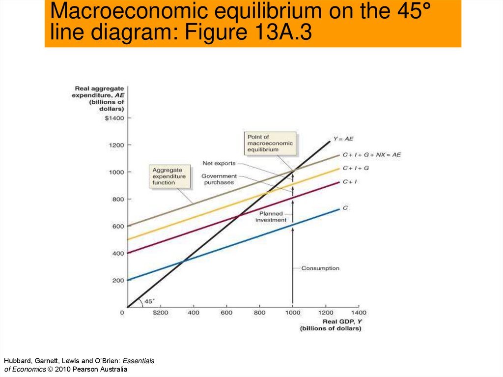
1995
1998
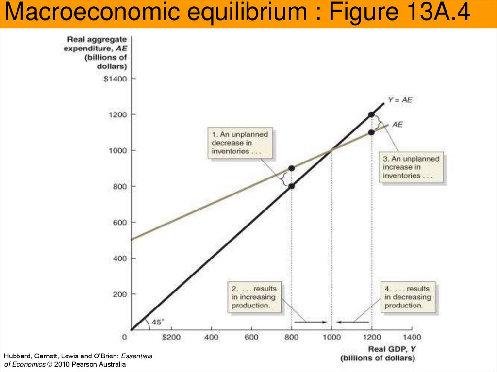
2001
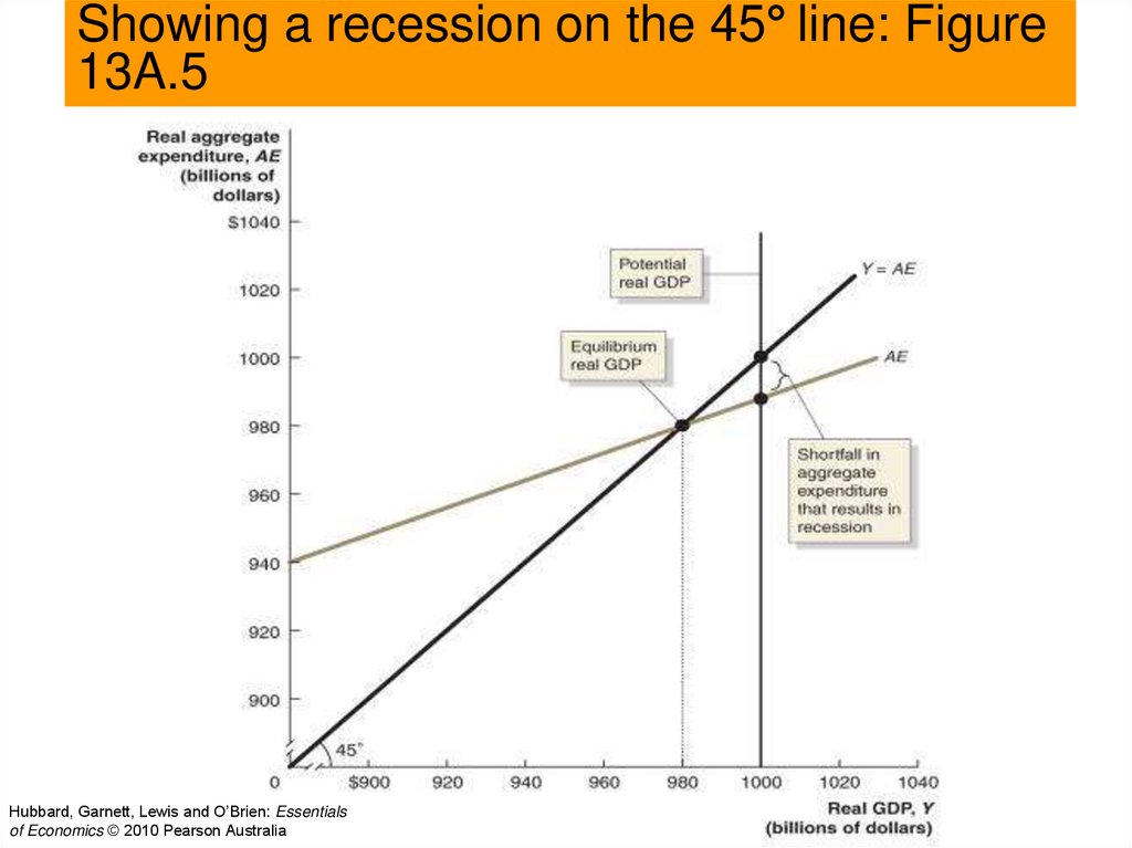
2004
2007
-1
-2
-3
Source: Australian Bureau of Statistics (2008),
Australian National Accounts, Cat. No. 5206.0.
Hubbard, Garnett, Lewis and O’Brien: Essentials of Economics © 2010 Pearson Australia

8. The Business Cycle

LEARNING OBJECTIVE 1
The Business Cycle
What happens during a business cycle?
Each business cycle is different, however
all share some similarities.
The end of an expansion is typically
associated with rising interest rates rising and
wages, and profits begin to fall.
A recession often begins with decreased
spending by firms on capital goods, and/or
decreased spending by households on new
houses and consumer durables.
Hubbard, Garnett, Lewis and O’Brien: Essentials of Economics © 2010 Pearson Australia

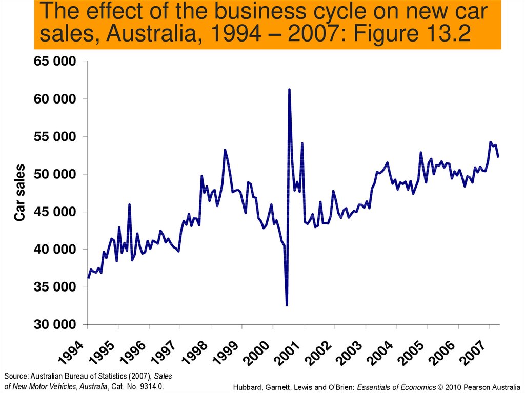
9. The Business Cycle

LEARNING OBJECTIVE 1
The Business Cycle
What happens during a business cycle?
The effect of the business cycle on car
sales.
Consumer durables are affected by the
business cycle more than non-durables.
People postpone buying durables, particularly
expensive items such as new cars, during a
recession.
Hubbard, Garnett, Lewis and O’Brien: Essentials of Economics © 2010 Pearson Australia

10.

The effect of the business cycle on new car
sales, Australia, 1994 – 2007: Figure 13.2
65 000
60 000
Car sales
55 000
50 000
45 000
40 000
35 000
19
94
19
95
19
96
19
97
19
98
19
99
20
00
20
01
20
02
20
03
20
04
20
05
20
06
20
07
30 000
Source: Australian Bureau of Statistics (2007), Sales
of New Motor Vehicles, Australia, Cat. No. 9314.0.
Hubbard, Garnett, Lewis and O’Brien: Essentials of Economics © 2010 Pearson Australia

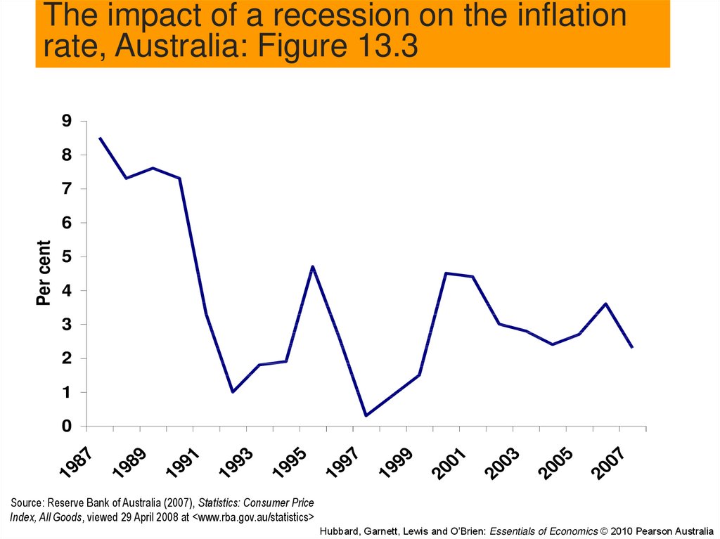
11. The Business Cycle

LEARNING OBJECTIVE 1
The Business Cycle
What happens during a business cycle?
The impact of a recession on the
inflation rate.
During economic expansions the inflation rate
usually increases.
Exception: If the expansion is due to rising
productivity levels and an expansion of potential
GDP.
During recessions the inflation rate usually
decreases.
Exception: The recession is caused by a supply
shock.
Hubbard, Garnett, Lewis and O’Brien: Essentials of Economics © 2010 Pearson Australia

12.

The impact of a recession on the inflation
rate, Australia: Figure 13.3
9
8
7
Per cent
6
5
4
3
2
1
07
20
05
20
03
20
01
20
99
19
97
19
95
19
93
19
91
19
89
19
19
87
0
Source: Reserve Bank of Australia (2007), Statistics: Consumer Price
Index, All Goods, viewed 29 April 2008 at <www.rba.gov.au/statistics>
Hubbard, Garnett, Lewis and O’Brien: Essentials of Economics © 2010 Pearson Australia

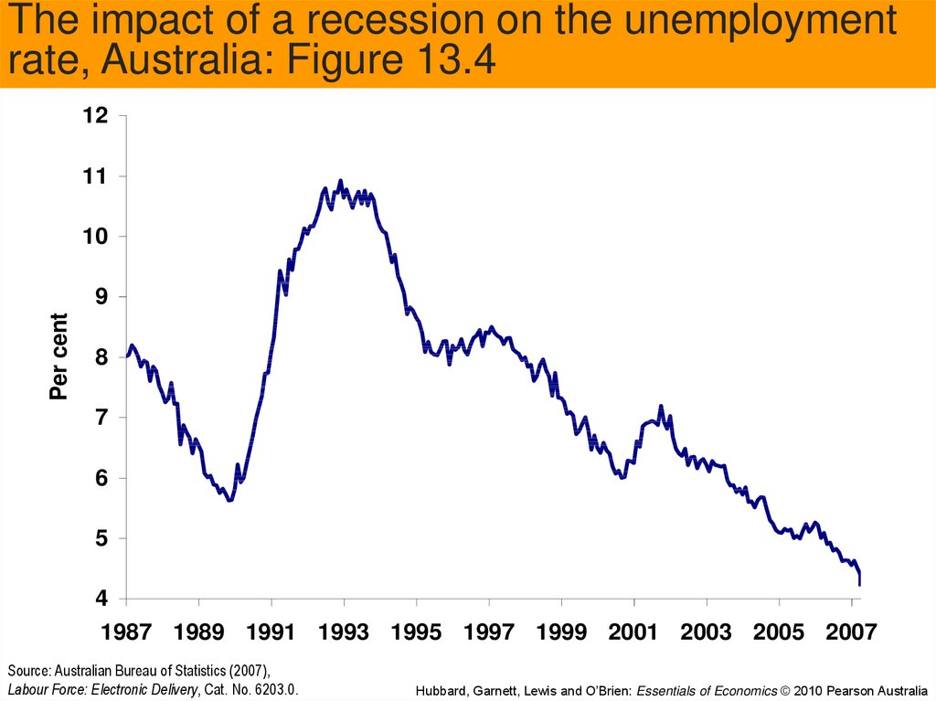
13. The Business Cycle

LEARNING OBJECTIVE 1
The Business Cycle
What happens during a business cycle?
The impact of a recession on the
unemployment rate.
Recessions cause the unemployment rate to
increase.
The rate of unemployment continues to rise
after the recession is over, because:
Discouraged workers re-enter the labour force.
Firms continue to operate below capacity after the
recession is over and may not re-hire workers for
some time.
Hubbard, Garnett, Lewis and O’Brien: Essentials of Economics © 2010 Pearson Australia

14.

The impact of a recession on the unemployment
rate, Australia: Figure 13.4
12
11
10
Per cent
9
8
7
6
5
4
1987 1989 1991 1993 1995 1997 1999 2001 2003 2005 2007
Source: Australian Bureau of Statistics (2007),
Labour Force: Electronic Delivery, Cat. No. 6203.0.
Hubbard, Garnett, Lewis and O’Brien: Essentials of Economics © 2010 Pearson Australia

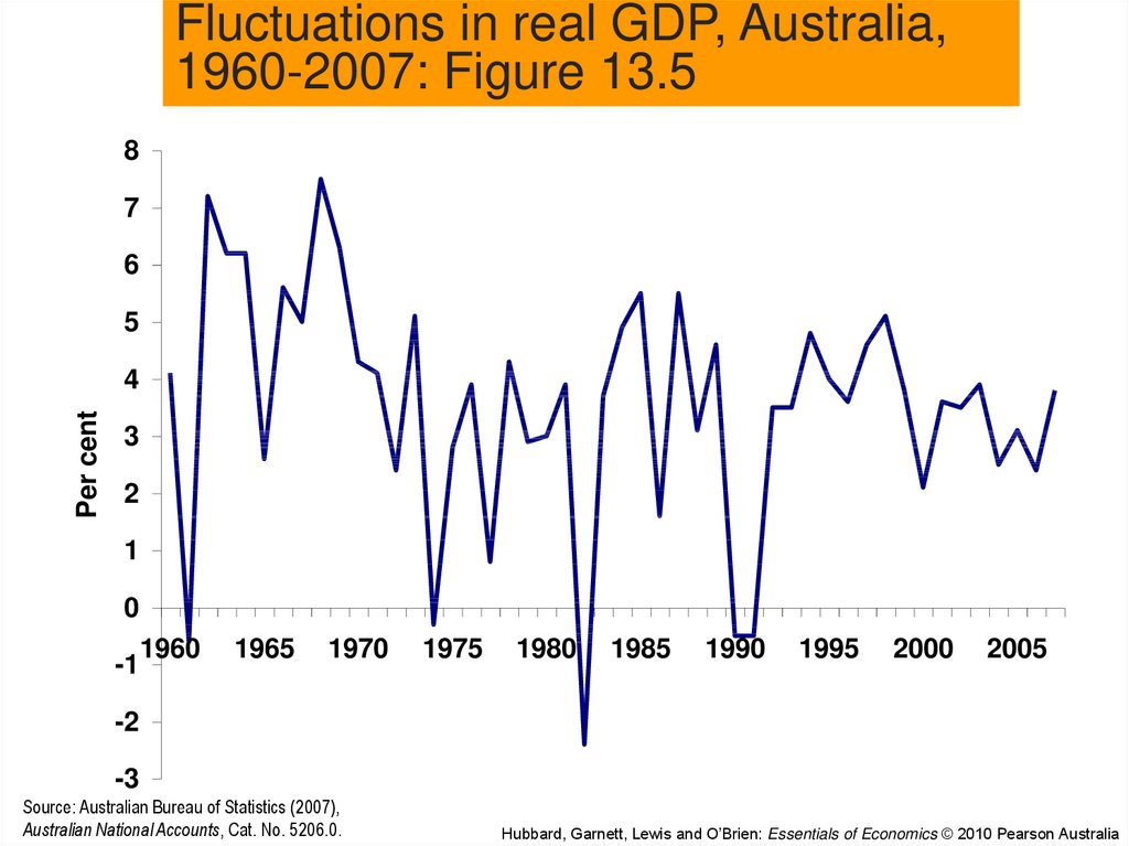
15. The Business Cycle

LEARNING OBJECTIVE 1
The Business Cycle
What happens during a business cycle?
Recessions are partly due to business
cycles and partly due to economic
shocks.
Oil price shock – OPEC.
1974:
1982/83: High real wages and inflation.
1990:
Government induced recession due
to high interest rates.
2008/09: World financial crisis – credit
shortage.
Hubbard, Garnett, Lewis and O’Brien: Essentials of Economics © 2010 Pearson Australia

16.

Fluctuations in real GDP, Australia,
1960-2007: Figure 13.5
8
7
6
5
Per cent
4
3
2
1
0
-1
1960
1965
1970
1975
1980
1985
1990
1995
2000
2005
-2
-3
Source: Australian Bureau of Statistics (2007),
Australian National Accounts, Cat. No. 5206.0.
Hubbard, Garnett, Lewis and O’Brien: Essentials of Economics © 2010 Pearson Australia

17. Aggregate Demand

LEARNING OBJECTIVE 2
Aggregate Demand
Aggregate demand and aggregate
supply model: A model that explains
short-run fluctuations in real GDP and the
price level.
Real GDP and the price level are
determined in the short run by the
intersection of the aggregate demand curve
and the short-run aggregate supply curve.
Hubbard, Garnett, Lewis and O’Brien: Essentials of Economics © 2010 Pearson Australia

18. Aggregate Demand

LEARNING OBJECTIVE 2
Aggregate Demand
Aggregate demand curve (AD): A
curve showing the relationship between the
price level and the quantity of real GDP
demanded by households, firms and the
government.
Short-run aggregate supply curve:
(SRAS): A curve showing the relationship in
the short-run between the price level and
the quantity of real GDP supplied by firms.
Hubbard, Garnett, Lewis and O’Brien: Essentials of Economics © 2010 Pearson Australia

19. Aggregate demand and aggregate supply: Figure 13.6

Price level
Short-run
aggregate
supply,
SRAS
100
Aggregate
demand, AD
0
$1000
Real GDP (billions of
dollars)
Hubbard, Garnett, Lewis and O’Brien: Essentials of Economics © 2010 Pearson Australia

20. Aggregate Demand

LEARNING OBJECTIVE 2
Aggregate Demand
Why is the aggregate demand curve
downward sloping?
1.
The wealth effect
2.
The interest rate effect
3.
How a change in the price level affects
consumption.
How a change in the price level affects
investment.
The international-trade effect
How a change in the price level affects net
exports.
Hubbard, Garnett, Lewis and O’Brien: Essentials of Economics © 2010 Pearson Australia

21. Aggregate Demand

LEARNING OBJECTIVE 2
Aggregate Demand
Shifts in the aggregate demand curve
versus movements along it.
The AD curve shows the relationship
between the price level and the quantity of
real GDP demanded, holding everything
else constant.
Changes in the price level are depicted as
movements up or down a stationary
aggregate demand curve.
Hubbard, Garnett, Lewis and O’Brien: Essentials of Economics © 2010 Pearson Australia

22. Aggregate Demand

LEARNING OBJECTIVE 2
Aggregate Demand
The variables that shift the aggregate
demand curve:
1.
Changes in government policies.
Examples: taxes; government purchases.
2.
Changes in the expectations of households
or firms.
3.
Changes in foreign variables.
Examples: exchange rates; relative income
levels between countries.
Hubbard, Garnett, Lewis and O’Brien: Essentials of Economics © 2010 Pearson Australia

23.

13.1
MAKING THE
CONNECTION
The effect of exchange
rates on sales
During some years, the
falling value of the
Australian dollar
against the New
Zealand dollar reduced
prices of Australian
exports to New
Zealand.
Hubbard, Garnett, Lewis and O’Brien: Essentials of Economics © 2010 Pearson Australia

24.

LEARNING OBJECTIVE 2
Determinants of Aggregate Demand
Explain whether each of the following will cause a
movement along or a shift of the Aggregate Demand
(AD) curve.
In each case, specify which of the four components of
AD will be impacted, and explain how.
Hubbard, Garnett, Lewis and O’Brien: Essentials of Economics © 2010 Pearson Australia

25.

LEARNING OBJECTIVE 2
Determinants of Aggregate Demand
a) Rising interest rates cause a drop in consumer
optimism as households become concerned about
their ability to meet mortgage payments.
b) An increase in the price level decreases the value
of superannuation accounts held by Australian
households to fund their retirement.
c) The Australian dollar falls in value against the US
dollar and other major currencies.
Hubbard, Garnett, Lewis and O’Brien: Essentials of Economics © 2010 Pearson Australia

26.

LEARNING OBJECTIVE 2
Determinants of Aggregate Demand
STEP 1: Review the material. This question is intended
to help differentiate between events that will cause a
change in aggregate quantity demanded, (a movement
along the aggregate demand curve), and a change in
aggregate demand (a shift in the AD curve). The
material is covered in the sections ‘Why is the aggregate
demand curve downward sloping?’, and ‘The variables
that shift the aggregate demand curve’.
Hubbard, Garnett, Lewis and O’Brien: Essentials of Economics © 2010 Pearson Australia

27.

LEARNING OBJECTIVE 2
Determinants of Aggregate Demand
STEP 2: Answering (a): Households become pessimistic
about the future. In order to ensure they can continue to
meet higher mortgage payments caused by rising
interest rates, consumers spend less in the present. The
AD curve will shift inwards to the left.
STEP 3: Answering (b): This is an example of a change
in the value of assets, or the wealth effect.
Superannuation accounts are one of the most important
assets for many Australians.
An increase in the price level decreases the real value of
superannuation funds.
Hubbard, Garnett, Lewis and O’Brien: Essentials of Economics © 2010 Pearson Australia

28.

LEARNING OBJECTIVE 2
Determinants of Aggregate Demand
Aggregate quantity demanded will decrease as
households spend less in order to contribute more to
their superannuation. This is reflected in an upward
movement along the AD curve.
STEP 4: Answering (c): A fall in the value of the
Australian dollar means it costs less in terms of other
currencies to buy Australian dollars, and hence also
goods, services and investments denominated in
Australian dollars. Net exports should therefore
increase, and this will be reflected in an increase in AD
– a shift to the right of the AD curve.
Hubbard, Garnett, Lewis and O’Brien: Essentials of Economics © 2010 Pearson Australia

29. Aggregate Supply

LEARNING OBJECTIVE 3
Aggregate Supply
The long-run aggregate supply curve
(LRAS): A curve showing the relationship in
the long run between the price level and the
quantity of real GDP supplied.
The long-run aggregate supply curve
shows that in the long run, increases in the
price level do not affect the level of real
GDP.
The long-run aggregate supply curve is a
vertical line at potential GDP.
Hubbard, Garnett, Lewis and O’Brien: Essentials of Economics © 2010 Pearson Australia

30. Aggregate Supply

LEARNING OBJECTIVE 3
Aggregate Supply
Shifts in the long-run aggregate supply
curve.
The LRAS curve shifts because potential
real GDP increases over time.
Increases in potential GDP (or economic
growth) are due to:
1.
An increase in resources.
2.
An increase in machinery and equipment.
3.
New technology.
Hubbard, Garnett, Lewis and O’Brien: Essentials of Economics © 2010 Pearson Australia

31. The long-run aggregate supply curve: Figure 13.7

Price level
LRAS2006 LRAS2007 LRAS2008
112
100
95
0
$1100
$1140
$1170
Real GDP
(billions of dollars)
Hubbard, Garnett, Lewis and O’Brien: Essentials of Economics © 2010 Pearson Australia

32. Aggregate Supply

LEARNING OBJECTIVE 3
Aggregate Supply
The short-run aggregate supply curve.
The SRAS is upward sloping, showing that
in the short-run firms will produce more in
response to higher prices.
The prices of inputs tends to rise more
slowly than the prices of final products.
Contracts make some wages and prices
‘sticky’.
Firms are often slow to adjust wages.
Menu costs make some prices sticky. Menu
costs are costs to firms of changing prices.
Hubbard, Garnett, Lewis and O’Brien: Essentials of Economics © 2010 Pearson Australia

33. Aggregate Supply

LEARNING OBJECTIVE 3
Aggregate Supply
Shifts in the short-run aggregate supply
curve versus movements along it.
The SRAS curve shows the short-run
relationship between the price level and
the quantity of goods and services firms
are willing to supply, holding everything
else constant.
Changes in the price level are depicted as
movements up or down a stationary shortrun aggregate supply curve.
Hubbard, Garnett, Lewis and O’Brien: Essentials of Economics © 2010 Pearson Australia

34. Aggregate Supply

LEARNING OBJECTIVE 3
Aggregate Supply
Variables that shift the SRAS curve.
1.
Expected changes in the future price level.
2.
Adjustments of workers and firms to errors
in past expectations about the price level.
3.
Unexpected changes in the price of an
important natural resource.
Hubbard, Garnett, Lewis and O’Brien: Essentials of Economics © 2010 Pearson Australia

35. How expectations of the future price level affect the short-run aggregate supply: Figure 13.8

Price level
1. If firms and workers
expect the price level to
be 3% higher in 2010
than in 2009 …
SRAS2010
SRAS2009
2. … the SRAS curve
will shift to the left to
reflect worker and firm
expectations of rising
costs.
103
100
0
$1000
Real GDP (billions of
dollars)
Hubbard, Garnett, Lewis and O’Brien: Essentials of Economics © 2010 Pearson Australia

36. Aggregate Supply

LEARNING OBJECTIVE 3
Aggregate Supply
Variables that shift the short-run and the
long-run aggregate supply curves.
1. Increases in the labour force and/or in
the capital stock, and/or in resources.
2. Technological change.
Hubbard, Garnett, Lewis and O’Brien: Essentials of Economics © 2010 Pearson Australia

37. Macroeconomic equilibrium in the long run and the short run

LEARNING OBJECTIVE 4
Macroeconomic equilibrium in
the long run and the short run
In long-run equilibrium, the aggregate
demand and short-run aggregate supply
curves intersect at a point along the
long-run aggregate supply curve.
Hubbard, Garnett, Lewis and O’Brien: Essentials of Economics © 2010 Pearson Australia

38. Long-run macroeconomic equilibrium: Figure 13.9

Price level
LRAS
SRAS
100
AD
0
$1000
Real GDP (billions of
dollars)
Hubbard, Garnett, Lewis and O’Brien: Essentials of Economics © 2010 Pearson Australia

39. Macroeconomic equilibrium in the long run and the short run

LEARNING OBJECTIVE 4
Macroeconomic equilibrium in
the long run and the short run
Recessions, expansions and supply
shocks.
The following analysis of the aggregate
demand and aggregate supply model
begins with a simplified case, using two
assumptions:
1.
The price level is currently at 100, and workers
and firms expect it to remain at 100 in the
future.
2.
Potential GDP is at $1000 billion and will
remain at that level in the future.
Hubbard, Garnett, Lewis and O’Brien: Essentials of Economics © 2010 Pearson Australia

40. Macroeconomic equilibrium in the long run and the short run

LEARNING OBJECTIVE 4
Macroeconomic equilibrium in
the long run and the short run
Recession
1.
The short-run effect of a decline in
aggregate demand.
2.
AD curve shifts left, and real GDP declines.
Adjustment back to potential GDP in the
long run.
Automatic adjustment mechanism: SRAS
curve shifts right, (which may take several
years).
Hubbard, Garnett, Lewis and O’Brien: Essentials of Economics © 2010 Pearson Australia

41. The short-run and long-run effects of a decrease in aggregate demand: Figure 13.10

Price level
1. A decline in
investment
shifts AD to the
left causing a
recession.
LRAS
SRAS2
96
2. As firms and workers
adjust to the price level
being lower than
expected, costs will fall,
and cause SRAS to shift
to the right.
A
100
98
SRAS1
B
C
AD2
0
3. Equilibrium moves from point
B back to potential GDP at
point C, with a lower price level.
$980 1000
AD1
Real GDP (billions of
dollars)
Hubbard, Garnett, Lewis and O’Brien: Essentials of Economics © 2010 Pearson Australia

42. Macroeconomic equilibrium in the long run and the short run

LEARNING OBJECTIVE 4
Macroeconomic equilibrium in
the long run and the short run
Expansion
1.
The short-run effect of an increase in
aggregate demand.
2.
AD curve shifts right, real GDP and the price
level rise.
Adjustment back to potential GDP in the
long run.
Automatic adjustment mechanism: SRAS
curve shifts left, (which may take a year or
more).
Hubbard, Garnett, Lewis and O’Brien: Essentials of Economics © 2010 Pearson Australia

43. The short-run and long-run effects of an increase in aggregate demand: Figure 13.11

Price level
1. An increase
in investment
shifts AD to the
right, causing
an inflationary
expansion.
LRAS
SRAS2
SRAS1
2. As firms and workers
adjust to the price level
being higher than
expected, costs will rise,
and cause SRAS to shift
to the left.
C
106
B
103
100
0
3. Equilibrium moves from point B
back to potential GDP at point C,
with a higher price level.
A
AD1
$1000 1030
AD2
Real GDP (billions of
dollars)
Hubbard, Garnett, Lewis and O’Brien: Essentials of Economics © 2010 Pearson Australia

44. Macroeconomic equilibrium in the long run and the short run

LEARNING OBJECTIVE 4
Macroeconomic equilibrium in
the long run and the short run
Supply shock: An unexpected event that
causes the short-run aggregate supply
curve to shift.
Stagflation: A combination of inflation and
recession, usually resulting from a supply
shock.
Hubbard, Garnett, Lewis and O’Brien: Essentials of Economics © 2010 Pearson Australia

45. Macroeconomic equilibrium in the long run and the short run

LEARNING OBJECTIVE 4
Macroeconomic equilibrium in
the long run and the short run
Supply shock
1.
The short-run effect of a supply shock.
2.
SRAS curve shifts left, real GDP falls and the
price level rises.
Adjustment back to potential GDP in the
long run.
SRAS curve shifts right, (which may take
several years).
Hubbard, Garnett, Lewis and O’Brien: Essentials of Economics © 2010 Pearson Australia

46. The short-run and long-run effects of a supply shock: Figure 13.12

Price
level
2. …moving short-run
equilibrium to point B,
with lower real GDP
and a higher price
level.
Price
level
LRAS
LRAS
SRAS2
SRAS1
104
100
B
SRAS1
104
A
1. An increase in oil
prices shifts SRAS
to the left …
100
B
A
AD
0
$970 1000
SRAS2
2. Equilibrium
moves from
point B
potential GDP
at the original
price level.
AD
Real GDP
(billions of
dollars)
(a) A recession with a rising price level –
the short-run effect of a supply shock.
0
$970 1000
Real GDP
(billions of
dollars)
(b) Adjustment back to potential GDP –
the long-run effect of a supply shock.
Hubbard, Garnett, Lewis and O’Brien: Essentials of Economics © 2010 Pearson Australia

47. The short-run and long-run effects of a supply shock: Figure 13.12

The short-run and long-run effects of a supply
1. The recession caused by the
shock: Figure 13.12
supply shock eventually leads to
Price
level
2. …moving short-run
equilibrium to point B,
with lower real GDP
and a higher price
level.
Price
level
LRAS
falling wages and prices, shifting
SRAS back to its original
position.
LRAS
SRAS2
SRAS1
104
100
B
SRAS1
104
A
1. An increase in oil
prices shifts SRAS
to the left …
100
B
A
AD
0
$970 1000
SRAS2
2. Equilibrium
moves from
point B to
potential GDP
at the original
price level.
AD
Real GDP
(billions of
dollars)
(a) A recession with a rising price level –
the short-run effect of a supply shock.
0
$970 1000
Real GDP
(billions of
dollars)
(b) Adjustment back to potential GDP –
the long-run effect of a supply shock.
Hubbard, Garnett, Lewis and O’Brien: Essentials of Economics © 2010 Pearson Australia

48.

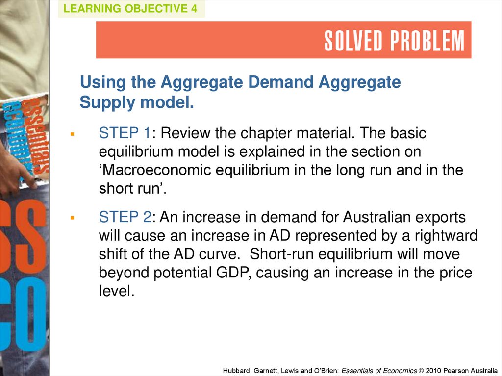
LEARNING OBJECTIVE 4
Using the Aggregate Demand Aggregate
Supply model.
Assume the economy is initially in equilibrium with
long-run aggregate supply (LRAS) constant. Now
suppose growing GDP in China and India leads to an
increase in demand and higher prices for Australian
resources. Explain both the initial change in
equilibrium and the longer term effect.
Hubbard, Garnett, Lewis and O’Brien: Essentials of Economics © 2010 Pearson Australia

49.

LEARNING OBJECTIVE 4
Using the Aggregate Demand Aggregate
Supply model.
STEP 1: Review the chapter material. The basic
equilibrium model is explained in the section on
‘Macroeconomic equilibrium in the long run and in the
short run’.
STEP 2: An increase in demand for Australian exports
will cause an increase in AD represented by a rightward
shift of the AD curve. Short-run equilibrium will move
beyond potential GDP, causing an increase in the price
level.
Hubbard, Garnett, Lewis and O’Brien: Essentials of Economics © 2010 Pearson Australia

50.

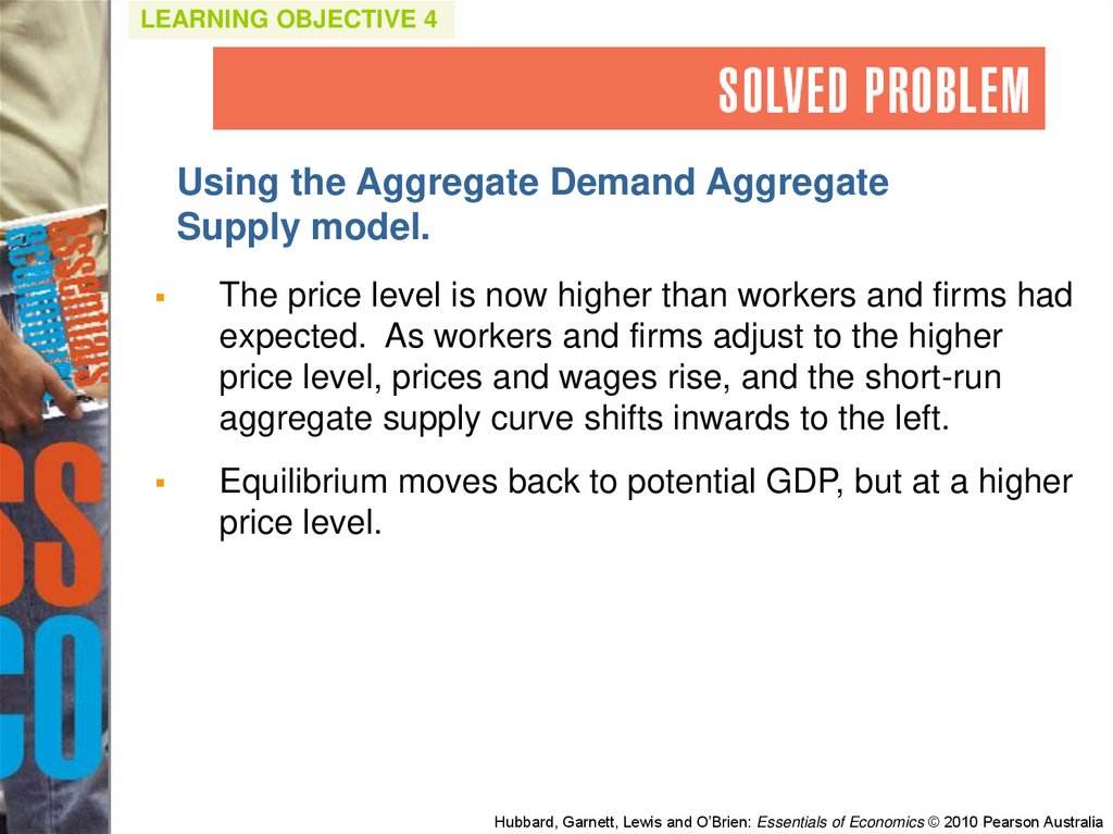
LEARNING OBJECTIVE 4
Using the Aggregate Demand Aggregate
Supply model.
The price level is now higher than workers and firms had
expected. As workers and firms adjust to the higher
price level, prices and wages rise, and the short-run
aggregate supply curve shifts inwards to the left.
Equilibrium moves back to potential GDP, but at a higher
price level.
Hubbard, Garnett, Lewis and O’Brien: Essentials of Economics © 2010 Pearson Australia

51. A dynamic aggregate demand and aggregate supply model

LEARNING OBJECTIVE 5
A dynamic aggregate demand and
aggregate supply model
A dynamic aggregate demand and aggregate
supply model can be created by making three
changes to the basic model:
1. Potential real GDP increases continually, shifting
the long-run aggregate supply curve to the right.
2. During most years the aggregate demand curve
will be shifting to the right.
3. Except during periods when workers and firms
expect high rates of inflation, the short-run
aggregate supply curve will be shifting to the
right.
Hubbard, Garnett, Lewis and O’Brien: Essentials of Economics © 2010 Pearson Australia

52. A dynamic aggregate demand and aggregate supply model: Figure 13.13

Price level
1. The economy
begins in
equilibrium at point
A with SRAS1 and
AD1 intersecting at
a point on LRAS1.
LRAS1
LRAS2 SRAS
1
2. During the course of a year,
increases in the labour force
and capital stock as well as
technological change cause a
shift from LRAS1 to LRAS2.
SRAS2
3. The same factors that cause the
LRAS curve to shift during the year
also cause the SRAS curve to shift.
A
B
100
5. The dynamic
AD-AS model
allows us to give a
more accurate
account of
changes in real
GDP and the price
level.
AD2
4. During the course of
the year, rising income
and population,
increasing investment,
and increasing
government purchases
cause the AD curve to
shift, and the economy
ends in a new
equilibrium at point B.
AD1
0
$1000
1030
Real GDP (billions of
dollars)
Hubbard, Garnett, Lewis and O’Brien: Essentials of Economics © 2010 Pearson Australia

53. Using dynamic aggregate demand and aggregate supply to understand inflation: Figure 13.14

Price level
LRAS1 LRAS2
104
100
B
A
SRAS1
SRAS2
1. If AD shifts to
the right more
than LRAS …
2. …the price
level rises.
AD1
AD2
0
$1000
1050
Real GDP (billions of
dollars)
Hubbard, Garnett, Lewis and O’Brien: Essentials of Economics © 2010 Pearson Australia

54.

13.2
MAKING THE
CONNECTION
Does rising productivity
growth reduce
employment?
New technology
and equipment
increases labour
productivity.
Hubbard, Garnett, Lewis and O’Brien: Essentials of Economics © 2010 Pearson Australia

55. An Inside Look

JB Hi-Fi reports
sales up 36% and
net profit after tax
up 56%.
Hubbard, Garnett, Lewis and O’Brien: Essentials of Economics © 2010 Pearson Australia

56. An Inside Look

Figure 1: Australian economic expansion between 2002 and 2007
Hubbard, Garnett, Lewis and O’Brien: Essentials of Economics © 2010 Pearson Australia

57. Key Terms

Aggregate demand and aggregate supply model
Aggregate demand curve (AD)
Business cycle
Long-run aggregate supply curve (LRAS)
Menu costs
Short-run aggregate supply curve (SRAS)
Stagflation
Supply shock
Hubbard, Garnett, Lewis and O’Brien: Essentials of Economics © 2010 Pearson Australia

58. Get Thinking!

At various times, the Australian dollar increases in value
against the US dollar and other major currencies. At the
same time, higher education continues as an important
component of Australia’s export revenue. The cost of
education in Australia therefore increases when the Australian
dollar rises relative to other currencies.
Discuss with your fellow students from other countries the
role the changing value of the Australian dollar played in their
decision to study in Australia.
Explain the impact that such changes have on the net export
component of aggregate demand, and hence aggregate
demand, ceteris paribus.
Hubbard, Garnett, Lewis and O’Brien: Essentials of Economics © 2010 Pearson Australia

59.

Check Your Knowledge
Q1. From a trough to a peak, the
economy goes through:
a.
The recession phase of the business
cycle.
b.
The expansion phase of the business
cycle.
c.
A contraction.
d.
A depression.
Hubbard, Garnett, Lewis and O’Brien: Essentials of Economics © 2010 Pearson Australia

60.

61.

Check Your Knowledge
Q2. During the early stages of a recovery:
a.
Firms usually rush to hire new
employees before other firms employ
them.
b.
Firms are usually reluctant to hire new
employees.
c.
The rate of unemployment surges
dramatically.
d.
The rate of unemployment decreases
dramatically.
Hubbard, Garnett, Lewis and O’Brien: Essentials of Economics © 2010 Pearson Australia

62. 63. Check Your Knowledge

Q3. The aggregate demand curve shows the
relationship between the price level and
the quantity of real GDP demanded by:
a. Households.
b. Firms.
c. The government.
d. All of the above.
Hubbard, Garnett, Lewis and O’Brien: Essentials of Economics © 2010 Pearson Australia

64. Check Your Knowledge

65. Check Your Knowledge

Q4. Which of the following factors do not
cause the aggregate demand curve to
shift?
a. A change in the price level.
b. A change in government policies.
c. A change in the expectations of households
and firms.
d. A change in foreign factors.
Hubbard, Garnett, Lewis and O’Brien: Essentials of Economics © 2010 Pearson Australia

66. Check Your Knowledge

67. Check Your Knowledge

Q5. How can government policies shift the
aggregate demand curve to the right?
a. By increasing personal income taxes.
b. By increasing business taxes.
c. By increasing government purchases.
d. All of the above.
Hubbard, Garnett, Lewis and O’Brien: Essentials of Economics © 2010 Pearson Australia

68. Check Your Knowledge

69. Check Your Knowledge

Q6. Which of the following statements is true?
a. In the long run, increases in the price level
result in an increase in real GDP.
b. In the long run, increases in the price level
result in a decrease in real GDP.
c. In the long run, increases in the price level result
in no change in real GDP.
d. In the long run, increases in the price level may
increase or decrease real GDP.
Hubbard, Garnett, Lewis and O’Brien: Essentials of Economics © 2010 Pearson Australia

70. Check Your Knowledge

71. Check Your Knowledge

Q7. Which of the following would shift both the
short-run and the long-run aggregate
supply curves?
a. A higher expected future price level.
b. An increase in the current price level.
c. A technological advance.
d. All of the above.
Hubbard, Garnett, Lewis and O’Brien: Essentials of Economics © 2010 Pearson Australia

72. Check Your Knowledge

73. Check Your Knowledge

Q8. Which of the following is usually the cause
of stagflation?
a. Reductions in government spending.
b. Increases in investment.
c. Printing money to finance government
expenditures.
d. An adverse supply shock.
Hubbard, Garnett, Lewis and O’Brien: Essentials of Economics © 2010 Pearson Australia

74. Check Your Knowledge

75. The aggregate expenditure model

APPENDIX
The aggregate expenditure
model
Aggregate Expenditure Model: A
macroeconomic model that focuses on the
relationship between total spending and
real GDP, assuming the price level is
constant.
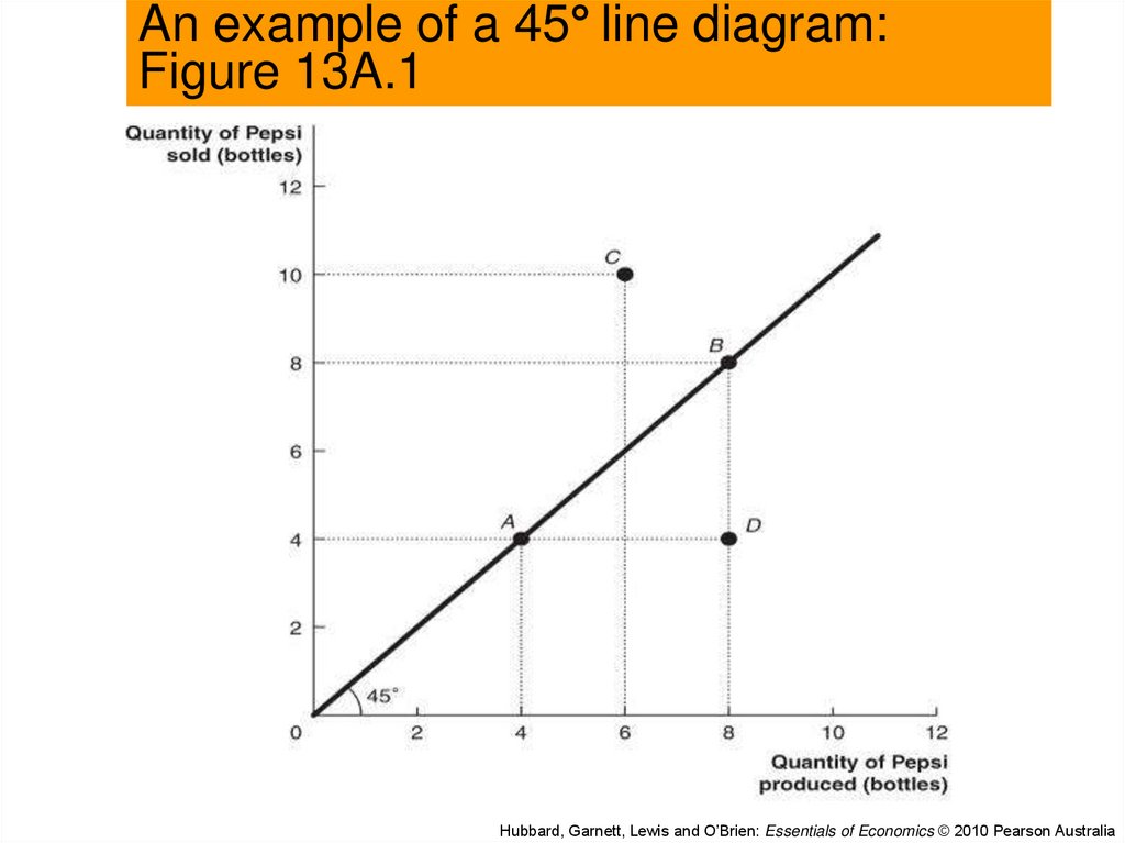
The model is composed of a graph called the
45° line diagram to illustrate macroeconomic
equilibrium.
Sometimes the model is also known as the
Keynesian cross diagram.
Hubbard, Garnett, Lewis and O’Brien: Essentials of Economics © 2010 Pearson Australia

76.

An example of a 45° line diagram:
Figure 13A.1
Hubbard, Garnett, Lewis and O’Brien: Essentials of Economics © 2010 Pearson Australia

77. The aggregate expenditure model

APPENDIX
The aggregate expenditure
model
Aggregate Expenditure (AE): The total
amount of spending in the economy: the
sum of consumption (C), planned
investment (I), government purchases (G),
and net exports (NX).
AE = C + I + G + NX
Hubbard, Garnett, Lewis and O’Brien: Essentials of Economics © 2010 Pearson Australia

78. Graphing macroeconomic equilibrium

APPENDIX
Graphing macroeconomic
equilibrium
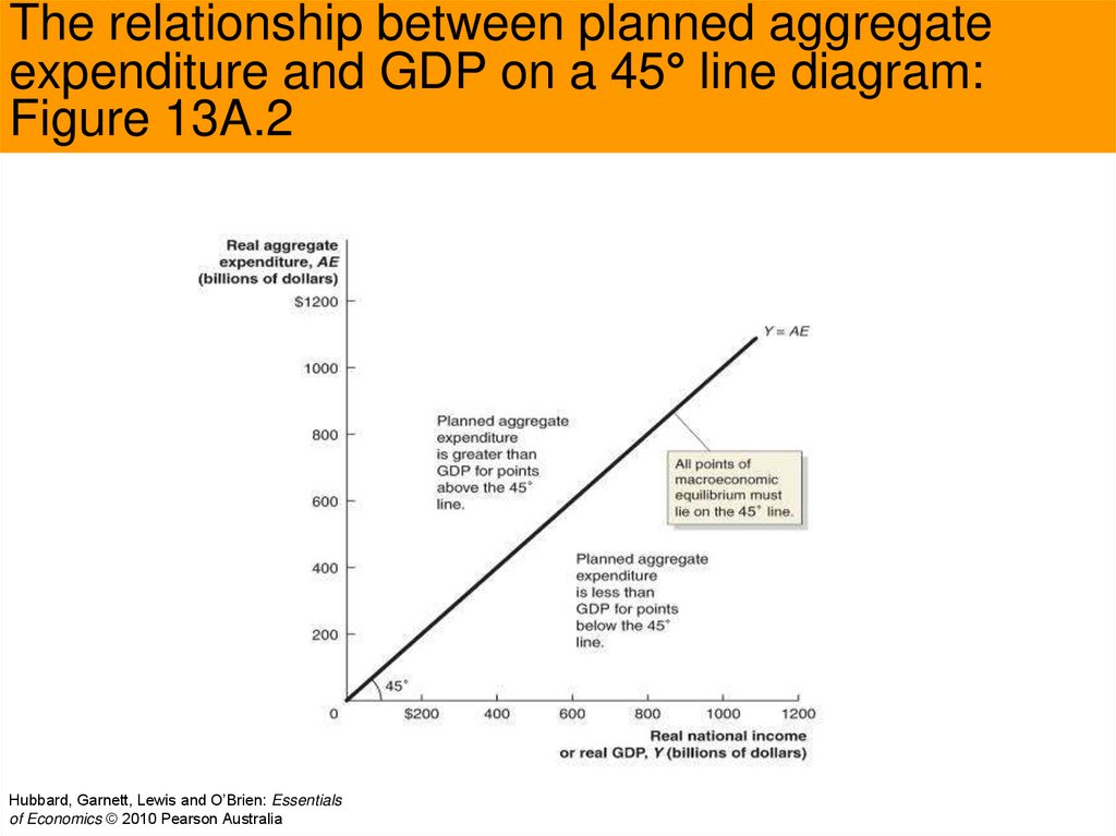
Using the 45° line diagram to illustrate
macroeconomic equilibrium.
The 45° line measures real national income
against planned real aggregate expenditure.
All points of macroeconomic equilibrium must
lie along the 45° line.
At points above the 45° line, aggregate
expenditures are greater than GDP.
At points below the 45° degree line,
aggregate expenditures are less than GDP.
Hubbard, Garnett, Lewis and O’Brien: Essentials of Economics © 2010 Pearson Australia

79.

The relationship between planned aggregate
expenditure and GDP on a 45° line diagram:
Figure 13A.2
Hubbard, Garnett, Lewis and O’Brien: Essentials
of Economics © 2010 Pearson Australia

80. The aggregate expenditure model

APPENDIX
The aggregate expenditure
model
Consumption function: The relationship
between consumption spending and
disposable income.
The consumption function intersects the
vertical axis on the 45° diagram at a point
above zero due to autonomous consumption.
Autonomous consumption: Consumption
that is independent of income.
Induced consumption: Consumption that
is determined by the level of income.
Hubbard, Garnett, Lewis and O’Brien: Essentials of Economics © 2010 Pearson Australia

81.

Macroeconomic equilibrium on the 45°
line diagram: Figure 13A.3
Hubbard, Garnett, Lewis and O’Brien: Essentials
of Economics © 2010 Pearson Australia

82. The aggregate expenditure model

APPENDIX
The aggregate expenditure
model
The AE line intersects the 45° line at
equilibrium real GDP.
At points above the 45° line, planned aggregate
expenditures are greater than GDP, inventories
will fall, leading to an increase in production.
At points below the 45° degree line, planned
aggregate expenditures are less than GDP,
firms will experience an unplanned increase in
inventories, leading to a decrease in production.
Hubbard, Garnett, Lewis and O’Brien: Essentials of Economics © 2010 Pearson Australia

83.

Macroeconomic equilibrium : Figure 13A.4
Hubbard, Garnett, Lewis and O’Brien: Essentials
of Economics © 2010 Pearson Australia

84. The aggregate expenditure model

APPENDIX
The aggregate expenditure
model
Showing a recession on the 45° line
diagram
Macroeconomic equilibrium can occur at any
point on the 45° line.
Ideal to have equilibrium occur at potential
real GDP.
If there is insufficient aggregate spending,
equilibrium will occur below potential real
GDP: the economy will be in a recession.
Hubbard, Garnett, Lewis and O’Brien: Essentials of Economics © 2010 Pearson Australia

85.

Showing a recession on the 45° line: Figure
13A.5
Hubbard, Garnett, Lewis and O’Brien: Essentials
of Economics © 2010 Pearson Australia

86. Check Your Knowledge

QA1. The idea of the aggregate expenditure
model is that, in any particular year, the
level of gross domestic product (GDP) is
determined mainly by:
a. The economy’s endowment of economic
resources and technology.
b. The level of interest rate for the economy as a
whole.
c. The level of aggregate expenditures.
d. The level of government expenditures.
Hubbard, Garnett, Lewis and O’Brien: Essentials of Economics © 2010 Pearson Australia

87. Check Your Knowledge

88. Check Your Knowledge

QA2. Which of the following statements is
correct?
a.
Actual investment and planned investment are
always the same.
b. Actual investment will equal planned
investment only when inventories rise.
c. Actual investment will equal planned
investment only when there is no unplanned
change in inventories.
d. Actual investment and planned investment only
when inventories decline.
Hubbard, Garnett, Lewis and O’Brien: Essentials of Economics © 2010 Pearson Australia

89. Check Your Knowledge

English Русский Rules