


 economics
Similar presentations:


Model of aggregate demand and aggregate supply. Topic 3
1.
TOPIC 3. MODEL OFAGGREGATE DEMAND AND
AGGREGATE SUPPLY
Plan
1. Aggregate demand and its model. Factors determining aggregate demand. AD
curve.
1а. Video – effects for a negative inclination of AD Video – effects for a negative
inclination of AD
2. Aggregate supply in the short and long run. Factors affecting the aggregate
supply. AS curve.
3. Macroeconomic equilibrium in the AD-AS model.
2.
1. Aggregate demand and its model. ADcurve
AGGREGATE DEMAND (AD) – is a schedule or curve
that shows the amounts of real output (real GDP)
that buyers collectively desire to purchase at each
possible price level.
The relationship between the price level (as
measured by the GDP price index) and the amount
of real GDP demanded is inverse or negative: When
the price level rises, the quantity of real GDP
demanded decreases; when the price level falls, the
quantity of real GDP demanded increases.
3.
1. Aggregate demand and its model. ADcurve
Aggregate demand is the planned expenditure in all
sectors of the economy. It contains four components:
1) expenditures of the private sector of the country
for consumption (C) and investment (I);
2) expenditures of the state for the purchase of
goods, payment for services and labor (G);
3) net exports of the country (NE) = export – import
AD = C+I+G+NE
4.
1. Aggregate demand and its model. ADcurve
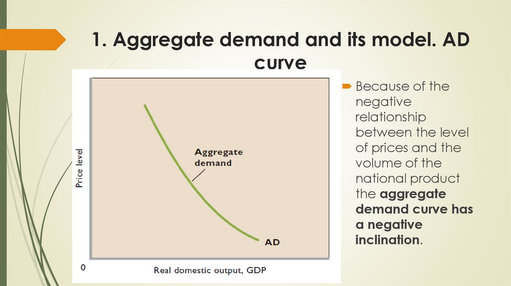
Because of the
negative
relationship
between the level
of prices and the
volume of the
national product
the aggregate
demand curve has
a negative
inclination.
5.
1. Aggregate demand and its model. ADcurve
AD factors are divided into:
Price related – factors that show how price of the
product influence AD
Non-price related – show how other price factors
except of price of the product influence AD
6.
1. Aggregate demand and its model. ADcurve
Price related factors:
1. Real-Balances Effect (wealth effect)- with the
growth of prices, decreases the purchasing power
of financial assets (cash); buyers reduce their
expenditure and aggregate demand is decreasing
and the opposite.
7.
1. Aggregate demand and its model. ADcurve
Price related factors:
2. Interest-Rate(Savings) Effect - with the increase of
the general level of prices, the demand for money
for the purchase of more expensive goods and
services increases, which leads to an increase in the
interest rate and a decrease in investments, which in
turn limits the aggregate demand.
p↑→ Мd ↑ → і↑→ І↓→АD↓
And vice versa:
p↓→ Мd ↓→ і↓→ І↑→ АD↑
8.
1. Aggregate demand and its model. ADcurve
3. Foreign Purchases Effect - the increase in the
general level of domestic prices in comparison with
the prices abroad leads to inflation, and,
consequently, the decrease in exports, and the
growth of imports, which will lead to a decrease in
net exports and a decrease in aggregate demand.
9.
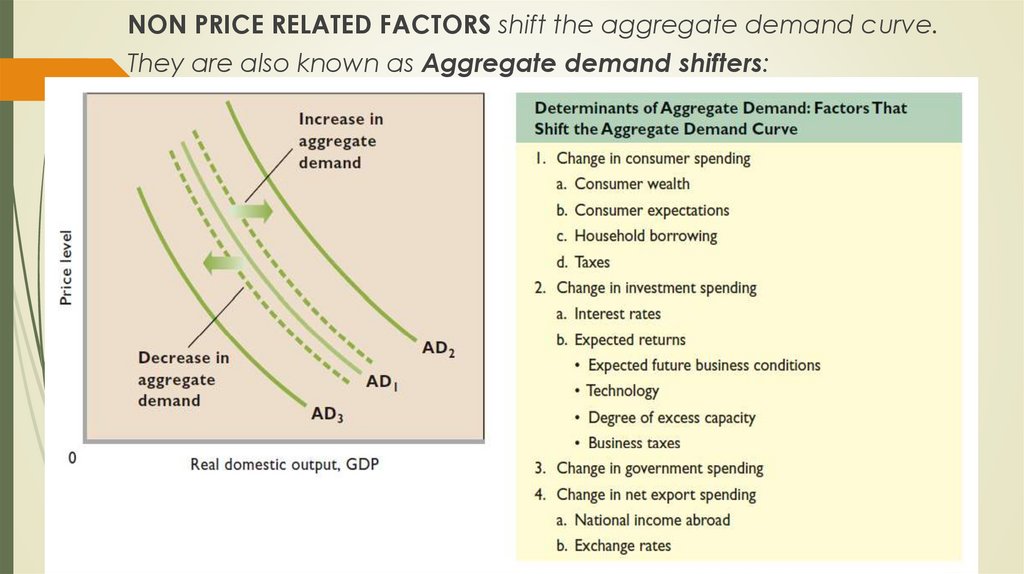
NON PRICE RELATED FACTORS shift the aggregate demand curve.They are also known as Aggregate demand shifters:
10.
1. Aggregate demand and its model. ADcurve
1. Change in consumer spending
Consumer Wealth - is the total dollar value of all assets owned by
consumers in the economy less the dollar value of their liabilities
(debts). Assets include stocks, bonds, and real estate. Liabilities
include mortgages, car loans, and credit card balances.
Household Borrowing. Consumers can increase their consumption
spending by borrowing. Doing so shifts the aggregate demand
curve to the right. By contrast, a decrease in borrowing for
consumption purposes shifts the aggregate demand curve to the
left.
11.
1. Aggregate demand and its model. ADcurve
1. Change in consumer spending
Consumer Expectations .When people expect their future
real incomes to rise, they tend to spend more of their
current incomes. Thus, current consumption spending
increases and the aggregate demand curve shifts to the
right.
Personal Taxes. Tax cuts shift the aggregate demand
curve to the right. Tax increases reduce consumption
spending and shift the curve to the left.
12.
1. Aggregate demand and its model. ADcurve
2. Investment Spending
Real Interest Rates Other things equal, an increase in real
interest rates will lower investment spending and reduce
aggregate demand.
Expected Returns Higher expected returns on investment
projects will increase the demand for capital goods and shift
the aggregate demand curve to the right.
Alternatively, declines in expected returns will decrease
investment and shift the curve to the left.
13.
1. Aggregate demand and its model. ADcurve
Expected returns, in turn, are influenced by several factors:
Expectations about future business conditions If firms are optimistic
about future business conditions, they are more likely to forecast high
rates of return on current investment and therefore may invest more
today.
Technology New and improved technologies enhance expected returns
on investment and thus increase aggregate demand.
Degree of excess capacity A rise in excess capacity— unused capital—
will reduce the expected return on new investment and hence
decrease aggregate demand. Other things equal, firms operating
factories at well below capacity have little incentive to build new
factories.
Business taxes An increase in business taxes will reduce after-tax profits
from capital investment and lower expected returns.
14.
1. Aggregate demand and its model. ADcurve
3. Government Spending
An increase in government purchases (for example, more
military equipment) will shift the aggregate demand curve to
the right, as long as tax collections and interest rates do not
change as a result. In contrast, a reduction in government
spending (for example, fewer transportation projects) will shift
the curve to the left.
15.
1. Aggregate demand and its model. ADcurve
4. Net Export Spending
Other things equal, higher U.S. exports mean an
increased foreign demand for U.S. goods.
So a rise in net exports shifts the aggregate demand
curve to the right. In contrast, a decrease in U.S. net
exports shifts the aggregate demand curve
leftward.
16.
1. Aggregate demand and its model. ADcurve
Causes of net exports change:
National Income Abroad Rising national income abroad
encourages foreigners to buy more products, some of which are
made in the United States. U.S. net exports thus rise, and the U.S.
aggregate demand curve shifts to the right.
Exchange Rates Changes in the dollar’s exchange rate—the price
of foreign currencies—may affect exports and therefore
aggregate demand.
Dollar depreciation increases net exports (imports go down;
exports go up) and therefore increases aggregate demand.
Dollar appreciation has the opposite effects: Net exports fall
(imports go up; exports go down) and aggregate demand
declines.
17.
2. Aggregate supply in the short and long run. Factorsaffecting the aggregate supply. AS curve.
AGGREGATE SUPPLY (AS) – is a schedule or curve
showing the relationship between the price level and
the amount of real domestic output that firms in the
economy produce.
The national economy can respond to changes in
aggregate demand either by increasing the volume
of the real product or by changing the price level.
18.
2. Aggregate supply in the short and long run. Factorsaffecting the aggregate supply. AS curve.
FULL EMPLOYMENT OUTPUT LEVEL (Potential GDP) is the
production level when all available resources are used
efficiently. It equals the highest level of production an
economy can sustain for the long-run.
It is also referred to as the full employment production,
natural level of output or long-run aggregate supply.
19.
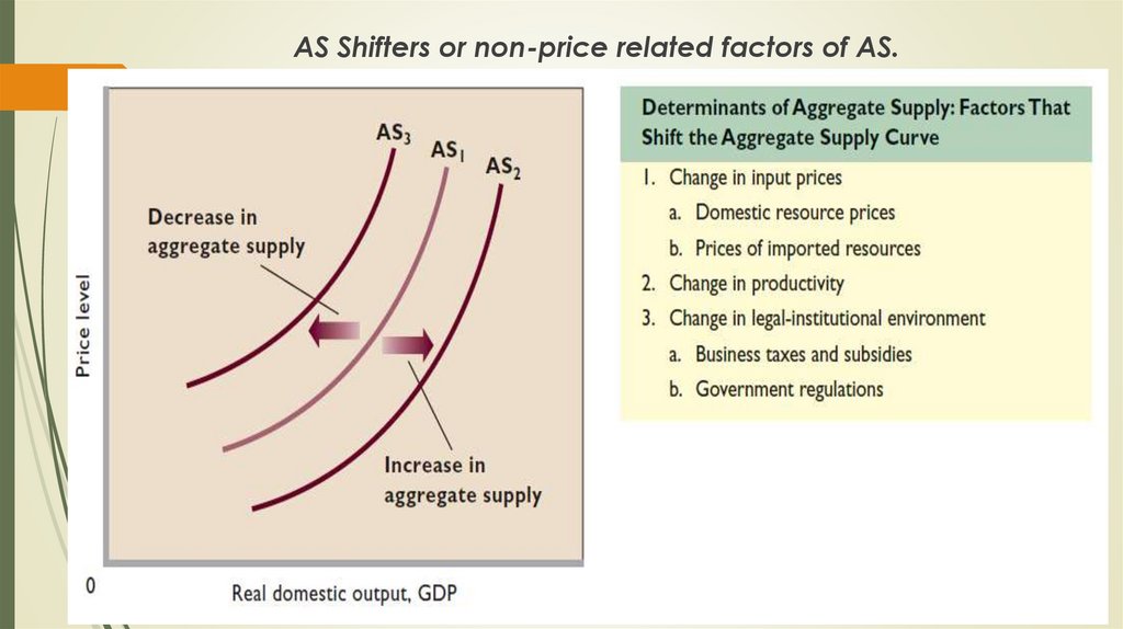
АS Shifters or non-price related factors of AS.20.
2. Aggregate supply in the short and long run. Factorsaffecting the aggregate supply. AS curve.
1. Input Prices
Input or resource prices—to be distinguished from the output
prices that make up the price level—are a major ingredient of
per-unit production costs and therefore a key determinant of
aggregate supply. These resources can either be domestic or
imported.
Domestic Resource Prices Wages and salaries make up about
75 percent of all business costs. Other things equal, decreases
in wages reduce per-unit production costs. So the aggregate
supply curve shifts to the right. Increases in wages shift the
curve to the left.
21.
2. Aggregate supply in the short and long run. Factorsaffecting the aggregate supply. AS curve.
Prices of Imported Resources
Just as foreign demand for national goods contributes to our
aggregate demand, resources imported from abroad (add to
national aggregate supply.
Added suppliesof resources—whether domestic or imported—
typically reduce per-unit production costs. A decrease in the
price of imported resources increases national aggregate
supply, while an increase in their price reduces national
aggregate supply.
22.
2. Aggregate supply in the short and long run. Factorsaffecting the aggregate supply. AS curve.
2. Change in productivity
Productivity- is a measure of the relationship between
a nation’s level of real output and the amount of
resources used to produce that output.
An increase in productivity enables the economy to
obtain more real output from its limited resources. It
does this by reducing the per-unit cost of output (perunit production cost).
23.
2. Aggregate supply in the short and long run. Factorsaffecting the aggregate supply. AS curve.
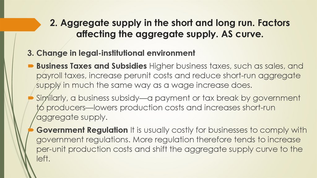
3. Change in legal-institutional environment
Business Taxes and Subsidies Higher business taxes, such as sales, and
payroll taxes, increase perunit costs and reduce short-run aggregate
supply in much the same way as a wage increase does.
Similarly, a business subsidy—a payment or tax break by government
to producers—lowers production costs and increases short-run
aggregate supply.
Government Regulation It is usually costly for businesses to comply with
government regulations. More regulation therefore tends to increase
per-unit production costs and shift the aggregate supply curve to the
left.
24.
The shape of the AS curve is interpreted differently inClassical and Keynesian theories.
Classical theory describes the economy in the long run. The analysis of the
aggregate supply in the classical theory is based on the following
conditions:
markets are competitive;
the volume of output depends only on the number of factors of
production (labor and capital) and technology and does not depend
on the price level;
changes in factors of production and technology are slow;
the economy operates at full employment output level;
prices and nominal wages - are flexible, their changes maintain the
balance in the markets.
The AS curve in the long run (LRAS) has vertical form at full employment
output level.
Any fluctuations in aggregate demand are reflected at the price level.
25.
2. Aggregate supply in the short and long run. Factorsaffecting the aggregate supply. AS curve.
26.
2. Aggregate supply in the short and long run. Factorsaffecting the aggregate supply. AS curve.
Keynesian theory considers the functioning of the economy in the
short run. The analysis of aggregate supply in the Keynesian theory is
based on the following conditions:
the economy operates under conditions of partial employment of
factors of production;
prices, nominal wages and other nominal values are relatively rigid,
slowly react to market fluctuations;
real values (output, employment, real wages, etc.) are more mobile,
react more quickly to market fluctuations.
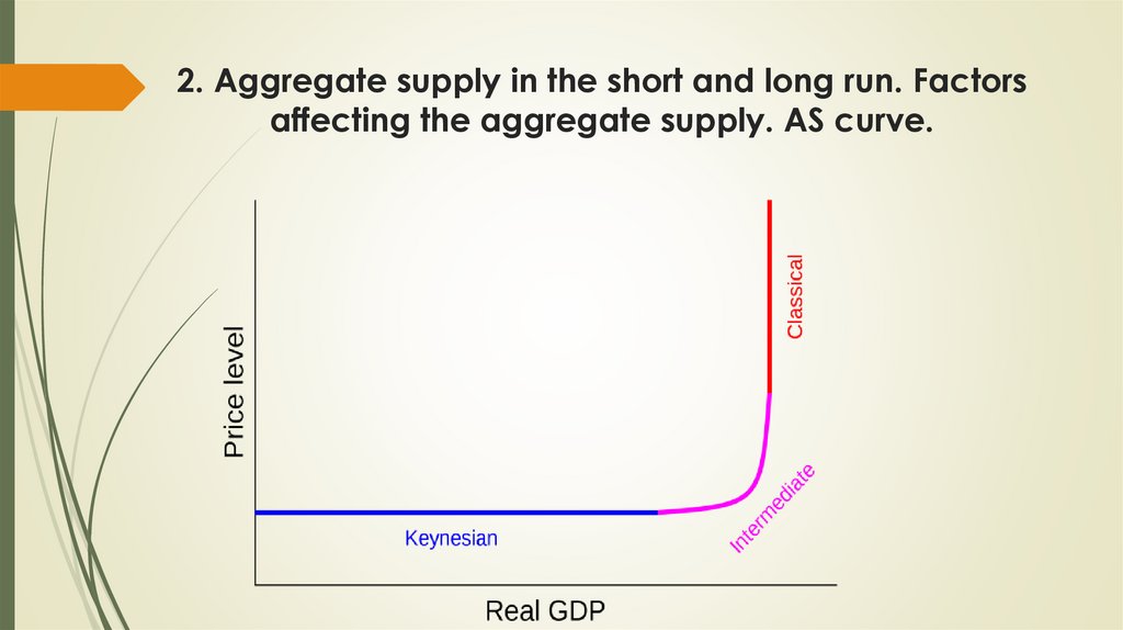
The short-term aggregate curve has two segments - the extreme
Keynesian and ascending
27.
2. Aggregate supply in the short and long run. Factorsaffecting the aggregate supply. AS curve.
The extreme Keynesian segment reflects the situation when the
economy is in decline, and therefore a significant proportion of
production capacity and labor is not used. In this segment, actual
production is smaller than full employment output level. The volume of
the national product is small, and therefore its increase does not lead
to the increase in prices level.
28.
2. Aggregate supply in the short and long run. Factorsaffecting the aggregate supply. AS curve.
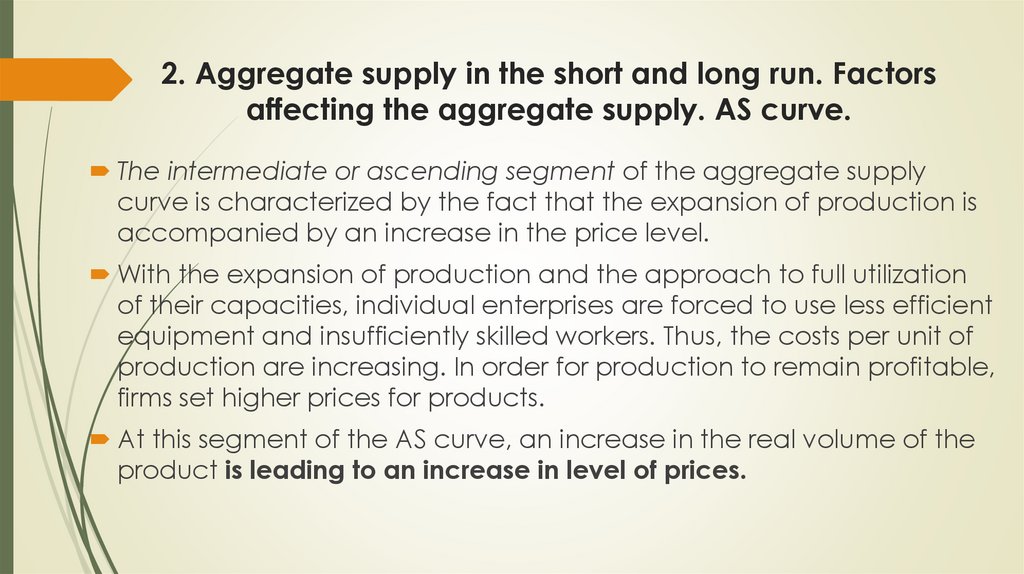
The intermediate or ascending segment of the aggregate supply
curve is characterized by the fact that the expansion of production is
accompanied by an increase in the price level.
With the expansion of production and the approach to full utilization
of their capacities, individual enterprises are forced to use less efficient
equipment and insufficiently skilled workers. Thus, the costs per unit of
production are increasing. In order for production to remain profitable,
firms set higher prices for products.
At this segment of the AS curve, an increase in the real volume of the
product is leading to an increase in level of prices.
29.
2. Aggregate supply in the short and long run. Factorsaffecting the aggregate supply. AS curve.
The vertical (classical) segment shows changes in GDP when it
reaches maximum, under full employment conditions (the level of
actual unemployment is equal to natural unemployment), and there is
no additional growth in real GDP, and therefore an inflationary rise in
prices occurs.
30.
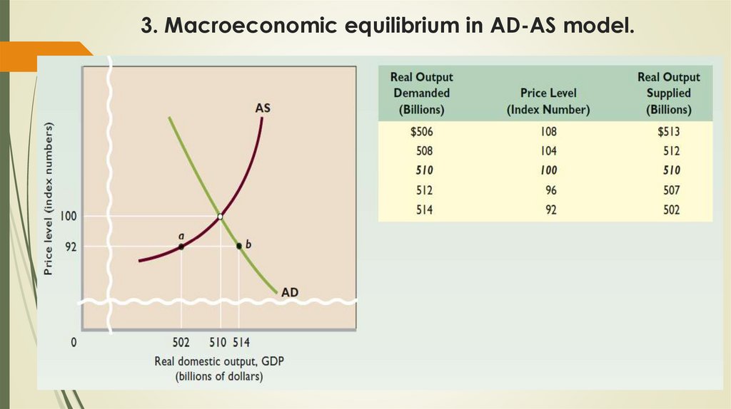
3. Macroeconomic equilibrium in AD-AS model.At the point of intersection of the curves of aggregate
demand and aggregate supply equilibrium level of prices and
the equilibrium volume of production of the national product
are achieved.
31.
3. Macroeconomic equilibrium in AD-AS model.32.
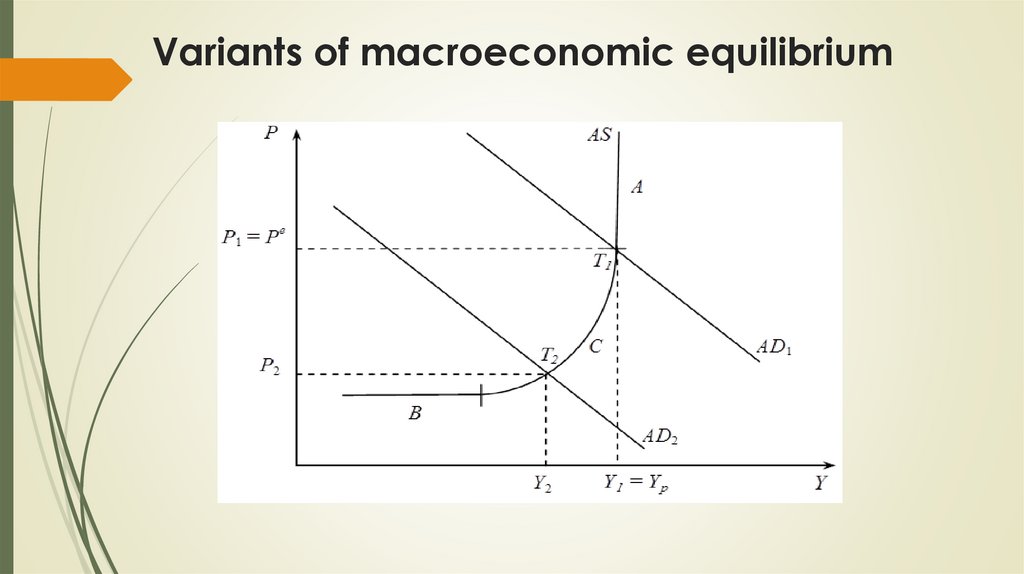
Variants of macroeconomic equilibrium33.
Variants of macroeconomic equilibrium1. If aggregate demand changes within the Keynesian
segment, then the growth of demand leads to an increase
in real domestic production and employment at constant
prices (B).
2. If aggregate demand grows in the intermediate period, it
leads to an increase in real GDP, prices and employment
(C)
3. If aggregate demand grows in the classic segment of AS, it
leads to inflationary growth in prices and nominal GDP with
constant real GDP (because, as already noted, it can not
grow more than the level of "full employment")(A)
34.
3. Macroeconomic equilibrium in AD-AS model.Different variants of macroeconomic equilibrium are possible depending
on employment conditions.
1. In the extreme Keynesian segment, where the aggregate supply
curve is horizontal, the change in aggregate demand mainly affects
the volume of national production, and the level of prices is stable.
2. In the classical segment, the AS curve becomes vertical, and
therefore the change in aggregate demand, for example, its
expansion, leads to higher prices, and real GDP is growing.
3. With the change in aggregate demand in the intermediate
segment of the aggregate supply, both real output and prices grow.