Unemployment rate

1.

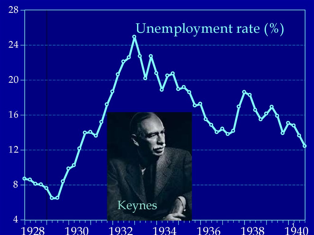
28
Unemployment rate (%)
24
20
16
12
8
Keynes
4
1928
1930
1932
1934
1936
1938
1
1940

2. Let’s review our voyage to date:

We have analyzed:
• Measuring economic activity
• Aggregate production functions and distribution
• Classical AS and AD (flexible w and p)
• Financial macro (including money)
• Open-economy macro
We now move on to
• Business cycles, Keynesian economics, and the ISLM model
2

3.

What picture do you have in mind when you think of
business cycles?
“Note that the pattern of cycles is irregular. No two business cycles are
quite the same. No exact formula, such as might apply to the
revolutions of the planets or of a pendulum, can be used to predict
the duration and timing of business cycles. Rather, in their
irregularities, business cycles more closely resemble the fluctuations
of the weather.” (Paul Samuelson)
3

4. Understanding business cycles

Major elements of cycles
–
–
–
–
short-period (1-3 yr) erratic fluctuations in output
pro-cyclical movements of employment, profits, prices
counter-cyclical movements in unemployment
appearance of “involuntary” unemployment in recessions
Historical trends
– lower volatility of output, inflation over time (until 2008)
– movement from stable prices to rising prices since WW II
4

5.

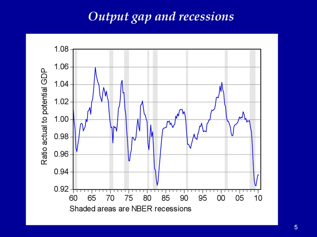
Output gap and recessions
Ratio actual to potential GDP
1.08
1.06
1.04
1.02
1.00
0.98
0.96
0.94
0.92
60 65 70 75 80 85 90 95
Shaded areas are NBER recessions
00
05
10
5

6.

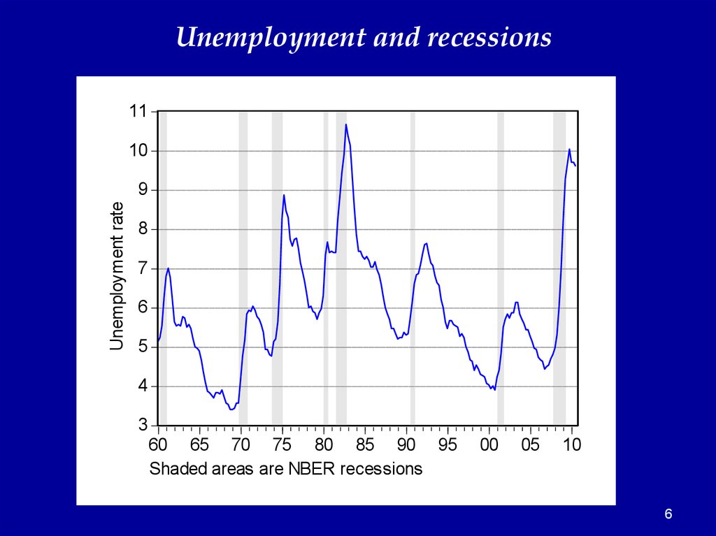
Unemployment and recessions
11
10
Unemployment rate
9
8
7
6
5
4
3
60 65 70 75 80 85 90 95
Shaded areas are NBER recessions
00
05
10
6

7.

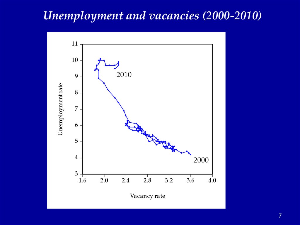
Unemployment and vacancies (2000-2010)
11
10
2010
Unemployment rate
9
8
7
6
5
4
3
2000
1.6
2.0
2.4
2.8
3.2
3.6
4.0
Vacancy rate
7

8.

So what’s the big problem for economics?
Many economists worry that there are no firm
“microeconomic foundations” for Keynesian business
cycle theory.
What should we do?
- throw out the theory?
- live with this inadequacy?
8

9.

Alternative Schools of Macroeconomics
Frictions in market institutions?
Market clearing
and perfect
competition
Rational
Frictions consumers
in indiv- and profit
maximizers
idual
Neoclassical (Solow,
Arrow-Debreu); new
classical macro; real
business cycles
decision Bounded
making? rationality, Original Keynes;
behavioral monetarist?
economics
9
Market frictions:
sticky prices and
wages; imperfect
competition
Neo-Keynesian (menu
costs and contract
theory); structuralism
Mainstream
Keynesian
9

10.

Alternative Schools of Macroeconomics
Frictions in market institutions?
Market clearing
and perfect
competition
Frictions Ultrain indiv- rational
idual
decision
making? Bounded
rationality
10
Market frictions:
sticky prices and
wages; imperfect
competition
This has been
the approach
up to now.
Classical model;
Neoclassical growth;
new classical macro;
real business cycles
10

11.

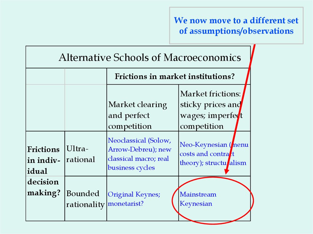
We now move to a different set
of assumptions/observations
Alternative Schools of Macroeconomics
Frictions in market institutions?
Market clearing
and perfect
competition
Neoclassical (Solow,
Arrow-Debreu); new
classical macro; real
business cycles
Frictions Ultrain indiv- rational
idual
decision
making? Bounded Original Keynes;
rationality monetarist?
Market frictions:
sticky prices and
wages; imperfect
competition
Neo-Keynesian (menu
costs and contract
theory); structuralism
Mainstream
Keynesian
11

12. Major approaches to business cycles

Classical: market clearing: supply-side cycles with vertical AS curve:
• Real business cycles: major active classical species today
Keynesian and offshoots: non-market clearing with non-vertical AS
• Essential to have non-classical AS
• Fixed or sticky p and w
• AD shifts affect output and employment
• Underlying theory incompletely understook – active area of research
Basic models in Keynesian approach
• “Keynesian cross” (Econ 116)
• AS-AD (Econ 116)
• IS-LM (Econ 122)
• Mankiw’s dynamic model (later)
• Open-economy in short run: Mundell-Fleming (later in course)
12

13.

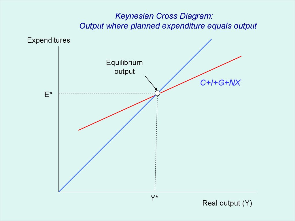
Keynesian Cross Diagram:
Output where planned expenditure equals output
Expenditures
Equilibrium
output
C+I+G+NX
E*
Y*
Real output (Y)
13

14.

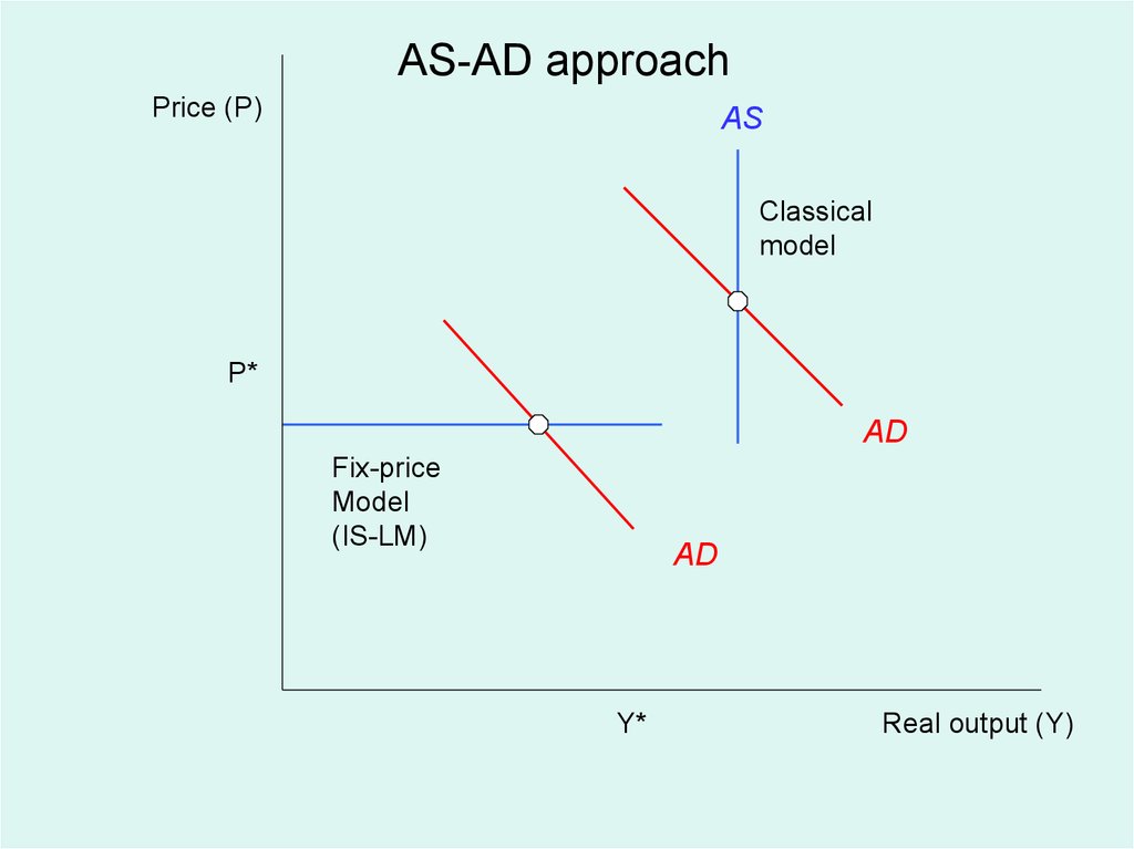
AS-AD approach
Price (P)
AS
Classical
model
P*
AD
Fix-price
Model
(IS-LM)
AD
Y*
Real output (Y)
14

15. IS-LM model

The major tool for showing the impact of monetary and
fiscal polices, along with the effect of various shocks, in a
short-run Keynesian situation.
Key assumptions
• Fixed prices (P=1)
• Unemployed resources (Y < potential Y = Mankiw’s natural Y)
• Closed economy (not essential and will be considered later)
15

16. The Founder of Macroeconomics

Gwendolen Darwin Raverat
16
16

17. Keynes on Why macroeconomics is difficult or Why the models are so confusing!

Professor Planck, of Berlin, the famous originator of the Quantum
Theory, once remarked to me that in early life he had thought of
studying economics, but had found it too difficult! Professor Planck
could easily master the whole corpus of mathematical economics in
a few days. But the amalgam of logic and intuition and the wide
knowledge of facts, most of which are not precise, which is required
for economic interpretation in its highest form is, quite truly,
overwhelmingly difficult.
(“Biography of Marshall,” Economic Journal, 1924)
17
17

18.

18

19. Where are we?

We are now attempting to understand the basic features of
business cycles.
Aggregate supply (AS) in this model is real simple: a horizontal
AS curve with p=1.
AD relies on the IS-LM model, which is a very simple twomarket model of the determinants of AD.
The two markets are
- goods (IS)
- financial (LM)
19

20. IS curve (expenditures)

Basic idea: describes equilibrium in goods market
Finds Y where planned I = planned S or planned
expenditure = planned output
Basic set of equations:
1.
2.
3.
4.
5.
Y=C+I+G
C = a + b(Y-T)
T = T0 + τ Y
[note assume income tax, τ = marginal tax rate]
I = I0 –dr
[note i = r because fixed P]
G = G0
20

21.

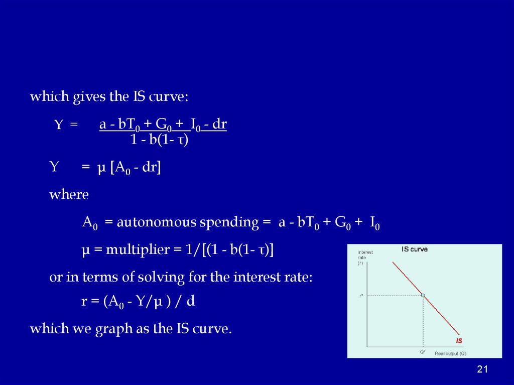
which gives the IS curve:
a - bT0 + G0 + I0 - dr
1 - b(1- τ)
Y =
Y
= μ [A0 - dr]
where
A0 = autonomous spending = a - bT0 + G0 + I0
μ = multiplier = 1/[(1 - b(1- τ)]
or in terms of solving for the interest rate:
r = (A0 - Y/μ ) / d
which we graph as the IS curve.
21

22. LM curve (financial markets)

• The LM curve represents equilibrium in financial markets, or where the
supply and demand for money are equilibrated.
• Ms determined by the central bank
Ms = M 0
interest
rate
(r)
IS-LM curve
LM
• Standard interest-elastic demand for money:*
Md = L(i, Y) = kY- hi
• Equilibrium in the money market is Md = Ms
• This leads to LM curve:
i = ( kY - M0 )/h
Real output (Q)
• Not the best way to understand financial markets;
will consider alternative approach later.
* Note that interest rate is nominal rate here to reflect the difference between the interest rate
on bonds and that on money.
22

23. Summary of IS-LM

1.
2.
3.
4.
Y≡C+I+G
C = a + b(Y-T)
T = T0 + τY
I = I0 – dr
5.
G = G0
6.
Ms = M0
7.
Md = L(i, Y) = kY- hi = kY- hr [r = i because zero inflation]
All this yields
hμ
Y* = ―――――― A0
dμk + h
dμ
+ ――――― M0
dμk + h
where
A0 = autonomous spending = a - bT0 + G0 + I0
μ = expenditure multiplier at constant r = 1/[(1 - b(1- τ)]
23

24. Overall Macroeconomic Equilibrium

• We now are looking for equilibrium of both markets. That is, when
both goods market and money market are in equilibrium.
• Closed economy and zero inflation (so i=r)
• This is the solution or intersection of IS and LM.
hμ
Y* = ―――――― A0
dμk + h
dμ
+ ――――― M0
dμk + h
• Impact of fiscal and monetary policy function of the different
parameters. Easiest to understand using the IS-LM diagram.
24

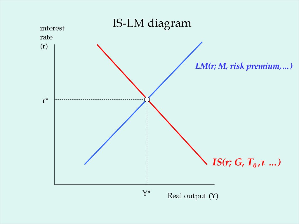
25.

interest
rate
(r)
IS-LM diagram
LM(r; M, risk premium,…)
r*
IS(r; G, T0 ,τ …)
Y*
Real output (Y)
25

26. SOME BASICS OF THE IS-LM MODEL

• Have two major kinds of shocks in business cycles:
– IS: investment, consumption, foreign trade, …
– LM: financial markets, monetary policy, exchange rates,…
• Because of monetary reaction, expenditure multiplier is almost
surely less than standard Keynesian multiplier due to crowding out.
– Proof: IS-LM multiplier = μ/[dμk/h + 1] < μ = simplest
multiplier
• Can usually diagnose shock by the relative movements of output
and interest rates (compare Vietnam War and 1979-82 on next slide)
26

27. Now several interesting cases

Case 1. A change in monetary policy
Note: by a monetary policy, we here mean a change in the money
supply (such as an open market operation), leading to a shift in the
LM curve.
27

28.

interest
rate
(r)
Monetary shift
LM
LM’
r*
r*’
IS
Y*
Y*’
Real output (Y)
28

29. More on financial issues…

Case 1A. A monetary crisis that increases risk premiums
- This important case will be covered next time when we do the Great
Depression (and today’s Great Recession).
29

30.

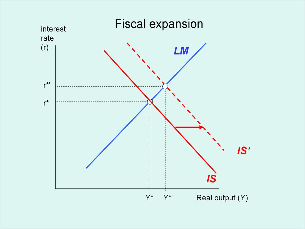
Case 2. What are the effects of fiscal policy?
A fiscal policy shift is change in purchases (G) or in taxes (T),
holding LM curve constant. See Figure.
30

31.

interest
rate
(r)
Fiscal expansion
LM
r*’
r*
IS’
IS
Y*
Y*’
Real output (Y)
31

32.

What is the multiplier?
interest
rate
(r)
LM
A
B
IS’
IS
μ
Real output (Y)
32

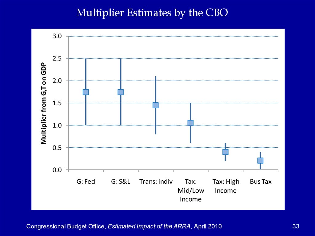
33.

Multiplier Estimates by the CBO
3.0
Multiplier from G,T on GDP
2.5
2.0
1.5
1.0
0.5
0.0
G: Fed
G: S&L
Trans: indiv
Tax:
Mid/Low
Income
Tax: High
Income
Congressional Budget Office, Estimated Impact of the ARRA, April 2010
Bus Tax
33

34.

Case 2b. The liquidity trap.
Today, this is taken to be where nominal interest rate is zero.
• The US in the mid-1930s
• Japan over last decade
• US in 2009-2010
34

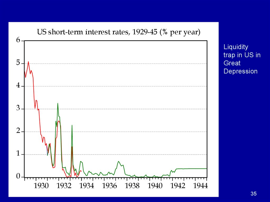
35.

6
US short-term interest rates, 1929-45 (% per year)
Liquidity
trap in US in
Great
Depression
5
4
3
2
1
0
1930
1932
1934
1936
1938
1940
1942
1944
35

36. Japan short-term interest rates, 1994-2006

Liquidity trap
from 1999 to
early 2006
36

37.

US today
Federal funds interest rate (% per annum)
20
16
Policy has
hit the
“zero lower
bound” this
year.
12
8
4
0
1975
1980
1985
1990
1995
2000
2005
2010
37

38.

interest
rate
(r)
Liquidity trap
IS
LM
LM’
Y*=Y*’
38

39. Heavy hitters in the Obama administration

Outgoing CEA head
Christina Romer
New CEA head
Austan Goolsbee
Economics czar
Larry Summers
Regulation: Cass Sunstein
3
Departed budget: Peter Orszag
39

40.

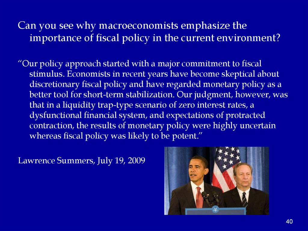
Can you see why macroeconomists emphasize the
importance of fiscal policy in the current environment?
“Our policy approach started with a major commitment to fiscal
stimulus. Economists in recent years have become skeptical about
discretionary fiscal policy and have regarded monetary policy as a
better tool for short-term stabilization. Our judgment, however, was
that in a liquidity trap-type scenario of zero interest rates, a
dysfunctional financial system, and expectations of protracted
contraction, the results of monetary policy were highly uncertain
whereas fiscal policy was likely to be potent.”
Lawrence Summers, July 19, 2009
40

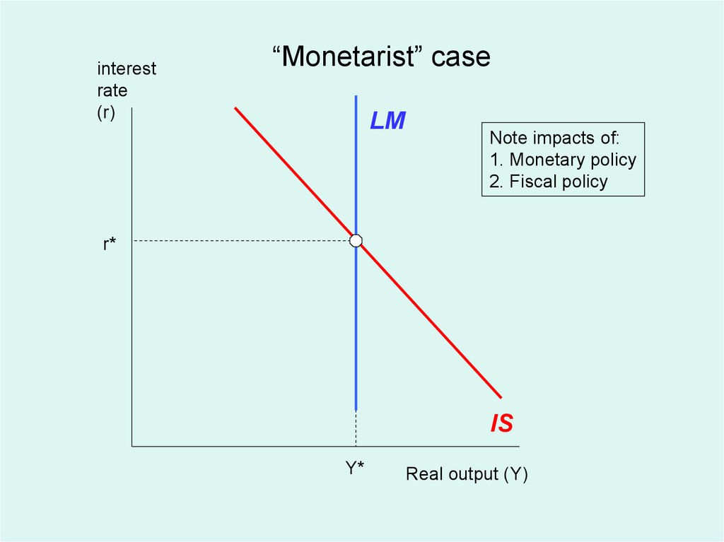
41. Case 3. Monetarism

• The monetarist regime: "Only money matters for output determination.“
(Milton Friedman).
• We can go back to quantity theory of money and prices:
PY = VM
• In monetarism view, velocity is constant . This would lead to a vertical LM
curve:
Md = kY – 0i
• Hence, equilibrating supply and demand for M yields:
Y =Ms/k
41

42.

interest
rate
(r)
“Monetarist” case
LM
Note impacts of:
1. Monetary policy
2. Fiscal policy
r*
IS
Y*
Real output (Y)
42

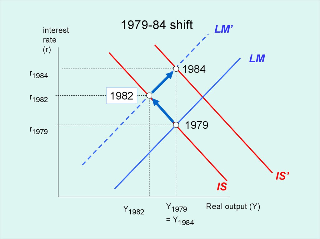
43. Important historical cases

Case 4. Changing the fiscal-monetary mix to stimulate or
depress investment
– A depressing example of tight money and loose fiscal
• New Fed chairman Volcker moved to tighten money and
wring inflation out of economy (1979 on)
• New President Reagan launched supply-side tax policies,
military buildup, leading to high deficits (1981 on)
• How did this affect fiscal-monetary mix
43

44.

interest
rate
(r)
1979-84 shift
LM’
LM
1984
r1984
r1982
1982
1979
r1979
IS’
IS
Y1982
Y1979
Real output (Y)
= Y1984
44

45. Important historical cases

Pro-growth policies
– The opposite would be to tighten fiscal policies and loosen
monetary policies.
– Make sure you understand how this would increase
investment and increase the growth in potential output.
45

46. Summary on IS-LM Model

This is the workhorse model for analyzing short-run
impacts of monetary and fiscal policy
Key assumptions:
- Fixed or rigid prices
- Unemployed resources
Now on to analysis of Great Depression in IS-LM
framework.
46