


")


")

")


")
")

")
")

")
")


 Priors")


: DSGE-VAR Approach")
")
")


")
")


")
")
")
")


")
, h=4, T0 =1985:4")
")

 mathematics
 economics
Similar presentations:


Forecasting with bayesian techniques MP
1.
Bayesian Models and Bayesian VARsJoint Vienna Institute/ IMF ICD
Macro-econometric Forecasting and Analysis
JV16.12, L08, Vienna, Austria, May 23, 2016
Presenter
Mikhail Pranovich
2.
Lecture Objectives• Introduce the idea of and rationale for Bayesian perspective and
Bayesian VARs
• Understand the idea of prior distribution of parameters,
Bayesian update and posterior distribution
• Become familiar with prior distributions for VAR parameters,
which allow for analytical representation of moments for
posterior distribution of VAR parameters
• Understand the idea and implementation of the DSGE-VAR
approach
2
3. Introduction: Two Perspectives in Econometrics
Let θ be a vector of parameters to be estimated using data
–
For example, if yt i.i.d. N(μ,σ2), then θ=[μ,σ2] are to be
estimated from a sample {yt}
Classical perspective:
–
there is an unknown true value for θ
–
we obtain a point estimator as a function of the data:
θˆ
Bayesian perspective:
–
θ is an unknown random variable, for which we have initial
uncertain beliefs - prior prob. distribution
–
we describe (changing) beliefs about θ in terms of probability
distribution (not as a point estimator!)
3
4. Outline
1. Why a Bayesian Approach to VARs?2. Brief Introduction to Bayesian Econometrics
3. Analytical Examples
Estimating a distribution mean
Linear Regression
4. Analytical priors and posteriors for BVARs
5. Prior selection in applications (incl. DSGE-VARs)
This training material is the property of the International Monetary Fund (IMF) and is intended for use in
IMF’s Institute for Capacity development (ICD) courses. Any reuse requires the permission of ICD.
4
5. Why a Bayesian Approach to VAR?
• Dimensionality problem with VARs:yt c A( L) yt 1 et ,
E{et et' } e
y contains n variables, p lags in the VAR
• The number of parameters in c and A is n(1+np), and the number of
parameters in Σ is n(n+1)/2
– Assume n=4, p=4, then we are estimating 78 parameters, with n=8, p=4, we
have 133 parameters
• A tension: better in-sample fit – worse forecasting performance
– Sims (Econometrica, 1980) acknowledged the problem:
“Even with a small system like those here, forecasting, especially over relatively long horizons,
would probably benefit substantially from use of Bayesian methods or other mean-squareerror shrinking devices…”
5
6. Why a Bayesian Approach to VAR? (2)
• Usually, only a fraction of estimated coefficients are statisticallysignificant
– parsimonious modeling should be favored
• What could we do?
– Estimate a VAR with classical methods and use standard tests to
exclude variables (i.e. reduce number of lags)
– Use Bayesian approach to VAR which allows for:
• interaction between variables
• flexible specification of the likelihood of such interaction
6
7. Combining information: prior and posterior
Bayesian coefficient estimates combine information in the
prior with evidence from the data
Bayesian estimation captures changes in beliefs about model
parameters
–
Prior: initial beliefs (e.g., before we saw data)
–
Posterior: new beliefs = evidence from data + initial
beliefs
7
8. Shrinkage
• There are many approachesparameterization in VARs
to
reducing
over-
– A common idea is shrinkage
• Incorporating prior information is a way of introducing
shrinkage
– The prior information can be reduced to a few parameters, i.e.
hyperparameters
8
9. Forecasting Performance of BVAR vs. alternatives
• BVAR providesbetter forecast of
Real GNP and
Inflation
Source: Litterman, 1986
9
10. Introduction to Bayesian Econometrics: Objects of Interest
Objects of interest:
–
Prior distribution: p ( )
–
Likelihood function: f ({ yt } | ) - likelihood of data at a given value of θ
–
Joint distribution (of unknown parameters and observables/data):
f ({ yt }, ) f ({ yt } | ) p ( )
–
–
Marginal likelihood:
f ({ yt })
Posterior distribution:
f ({ y }, )d f ({ y } | ) p ( ) d
t
t
f ({ yt }, ) f ({ yt } | ) p ( )
p ( | { yt })
f ({ yt })
f ({ yt })
i.e. what we learned about the parameters
(1) having
prior and (2) observing the
data
10
11. Bayesian Econometrics: Objects of Interest (2)
The marginal likelihood…
f ({ yt })
f ({ y }, )d f ({ y } | ) p ( )d
t
t
…is independent of the parameters of the model
Therefore, we can write the posterior as proportional to prior
and data:
p ( | { yt }) f ({ yt } | ) p ( )
We combine data & prior to get the posterior
11
12. Bayesian Econometrics: maximizing criterion
• For practical purposes, it is useful to focus on the criterion:C ( ) log f ({ yt } | ) log( p ( ))
–
Traditionally, priors that let us obtain analytical expressions for
the posterior would be needed
–
Today, with increased computer power, we can use any prior
and likelihood distribution, as long as we can evaluate them
numerically
Then we can use Markov Chain Monte-Carlo (MCMC) methods to simulate the
posterior distribution (not covered in this lecture)
12
13. Bayesian Econometrics : maximizing criterion (2)
Maximizing C( ) gives the Bayes mode. In some cases (i.e.
Normal distributions) this is also the mean and the median
The criterion can be generalized to:
C ( ) (1 ) log f ({ yt } | ) log( p ( ))
λ controls relative importance of prior information vs. data
13
14. Analytical Examples
• Let’s work on some analytical examples:1. Sample mean
2. Linear regression model
14
15. Estimating a Sample Mean
• Let yt i.i.d. N(μ,σ2), then the data density function is:1
1 T
2
f ( y | , )
exp{
(
y
)
}
t
2 T /2
2
(2 )
2 t 1
2
where y={y1,…yT}
• For now: assume variance σ2 is known (certain)
• Assume the prior distribution of mean μ is normal, μ N(m,σ2/ν):
( m) 2
f ( ; )
exp{
}
2
1/ 2
2
(2 / v)
2( / v)
2
1
where the key parameters of the prior distribution are m and ν
15
16. Estimating a Sample Mean
The posterior of μ:
f ( y | ; 2 ) f ( ; 2 )
f ( | y; )
f ( y ; 2 )
2
…has the following analytical form
( m* ) 2
1
f ( | y; )
exp 2
2
1/ 2
[2 /( T )]
2
/(
T
)
2
with
v
T
m (
)m (
) y,
v T
v T
*
1 T
y yt
T t 1
So, we “mix” prior m and the sample average (data)
• Note:
– The posterior distribution of μ is also normal: μ N(m*,σ2/{ν+T})
– Diffuse prior: ν→0 (prior is not informative, everything is in data)
– Tight prior: ν→ ∞ (data not important, prior is rather informative) 16
17. Estimating a Sample Mean: Example
• Assume the true distribution is Normal yt~N(3,1)– So, μ=3 is known to… God
• A researcher (one of us) does not know μ
– for him/her it is a normally distributed random variable μ~N(m,1/v)
• The researcher initially believes that m=1 and ν=1, so his/her prior
is μ~N(1,1)
0.4
0.35
0.3
0.25
0.2
0.15
0.1
0.05
0
4
2
0
2
4
6
8
10
17
18. Posterior with prior N(1,1)
• Compute the posterior distribution as sample size increases4.5
Prior
Post. T=10
Post .T=50
Post. T=100
4
3.5
• Already after 10 draws we get
closer to μ=3
• After 50 and 100:
3
2.5
– the mean of the distribution gets
closer to 3
2
1.5
– the dispersion is smaller
1
0.5
0
4
2
0
2
4
6
8
10
18
19. Posterior with Prior N(1,1/50)
• Then, we look at more informative (tight) prior and set ν =50(higher precision)
5
• The picture is different here
Prior
Post. T=10
Post .T=50
Post. T=100
4.5
4
• After 10 and 50 draws we still are quite
far from μ=3 … although we get closer
3.5
3
• Why?...
2.5
• Our prior was m=1, but this time it is
tighter (v=50 instead of v=1)
2
1.5
– i.e. harder to change based on observed
data
1
0.5
0
4
2
0
2
4
6
8
10
19
20. Examples: Regression Model I
• Linear Regression model:where ut i.i.d. N(0,σ2)
yt xt' ut
• Assume:
– β is random and unknown
– but σ2 is fixed and known
• Convenient matrix representation
Y X U
where
y1
Y ... ,
yT
1 x11
X ... ...
1 x1T
... xk 1
1
u1
... ... , ... , U ...
k
uT
... xkT
• The density function for data is:
1
1 T
f ( y | , X , )
exp{ 2 ( yt xt' ) 2 }
2 T /2
(2 )
2 t 1
1
(Y X )' (Y X )
exp{
}
(2 2 )T / 2
2 2
2
20
21. Examples: Regression Model I (2)
Assume that the prior mean of β has multivariate Normal distribution
N(m,σ2M):
ï (β m)'M 1 (β m) ï
1
1/2
f ( ; )
|M| exp
2 K /2
(2 )
2 2
ï
ï
2
where the key parameters of the prior distribution are m and M
Bayesian rule states:
f ( y | , X ; 2 ) f ( ; 2 ) f ( | y , X ; 2 ) f ( y | X ; 2 )
f ( y | , X ; 2 ) f ( ; 2 )
f ( | y , X ; )
f ( y | X ; 2 )
2
i.e., the posterior of β is proportional to the product of the data
density of data and prior
f ( | y , X ; 2 ) f ( y | , X ; 2 ) f ( ; 2 )
21
22. Examples: Regression Model I (3)
• We mix information – densities of data and prior – to getposterior distribution!
f ( | y , X ; 2 ) f ( y | , X ; 2 ) f ( ; 2 )
• Result: the density function of β is…
1
1
( m* )' ( M 1 X ' X )( m* )
1
2
f ( | y , X ; )
| M X ' X | exp{
}
(2 2 ) k / 2
2 2
2
• … which means that the posterior distribution is again (!) normal
~ N ( m* , 2 M * )
• with the mean and variance
m* ( M 1 X ' X ) 1 ( M 1m X ' y )
2 M * 2 ( M 1 X ' X ) 1
22
23.
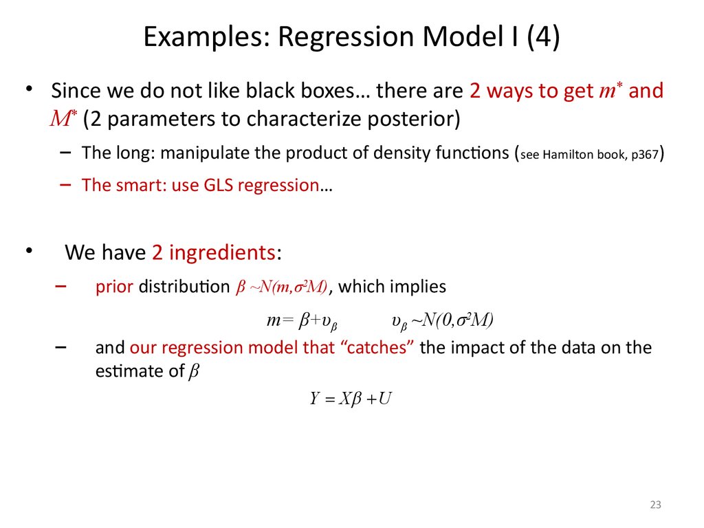
Examples: Regression Model I (4)• Since we do not like black boxes… there are 2 ways to get m* and
M* (2 parameters to characterize posterior)
– The long: manipulate the product of density functions ( see Hamilton book, p367)
– The smart: use GLS regression…
We have 2 ingredients:
–
prior distribution β ~N(m,σ2M), which implies
–
m= β+υβ
υβ ~N(0,σ2M)
and our regression model that “catches” the impact of the data on the
estimate of β
Y X U
23
24.
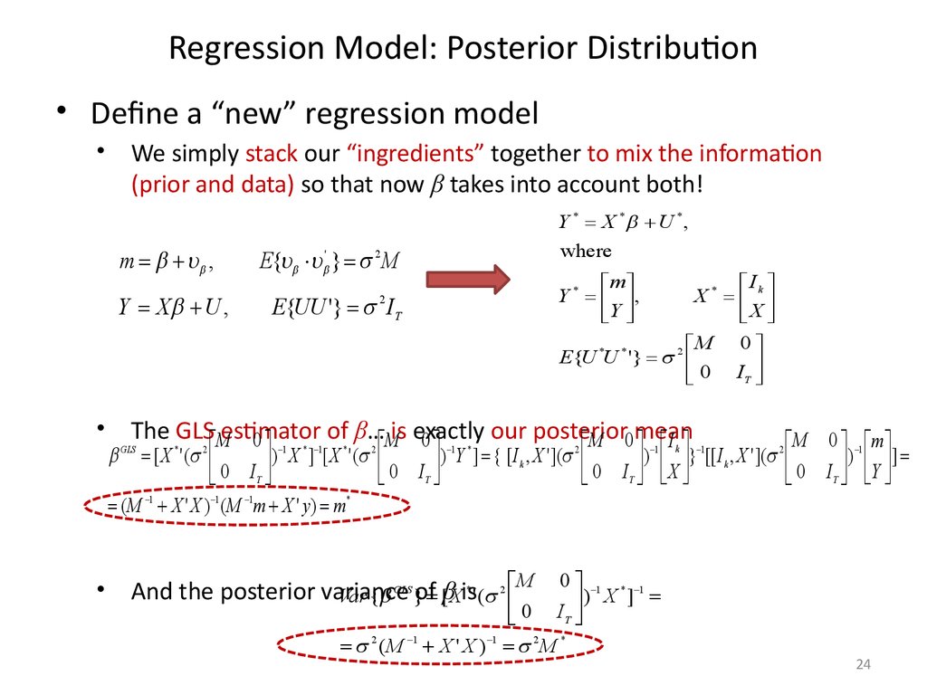
Regression Model: Posterior Distribution• Define a “new” regression model
We simply stack our “ingredients” together to mix the information
(prior and data) so that now β takes into account both!
m ,
Y X U ,
Y * X * U * ,
where
E{ ' } 2 M
m
Y * ,
Y
I
X* k
X
M 0
E{U *U * '} 2
0 IT
E{UU '} I T
2
The GLS Mestimator
of β… Mis exactly
our posterior
0
0
M 0mean
I
1
* 1
*
2
[ X * ' ( 2
)
X
]
[
X
'
(
0
0 IT
( M 1 X ' X ) 1 (M 1m X ' y ) m*
GLS
1 *
2
)
Y
]
{
[
I
,
X
'
](
k
0
IT
M 0 1 m
k
1
1
2
)
}
[[
I
,
X
'
](
k
0 I ) Y ]
IT X
T
M 0 1 * 1
0 I ) X ]
T
2
1
1
2
*
(M X ' X ) M
And the posterior variance
Var { }of [βXis' (
GLS
*
2
24
25. Examples: Regression Model II
• So far the life was easy(-ier), in the linear regression modelY X U
• β was random and unknown, but σ2 was fixed and known
• What if σ2 is random and unknown?..
• Bayesian rule states:
f ( , 2 | y, X ) f ( y | , X ; 2 ) f ( y | , X ; 2 ) f ( | 2 ) f ( 2 )
• i.e., the posterior of β and σ2 is proportional to the product of
the density of data, prior of β (given σ2) and prior of σ2
f ( y | , X ; 2 ) f ( | 2 ) f ( 2 )
f ( , | y , X )
f ( y | , X ; 2 )
2
f ( , 2 | y, X ) f ( y | X , , 2 ) f ( | 2 ) f ( 2 )
25
26. Examples: Regression Model II ()
• To manipulate the productf ( , 2 | y, X ) f ( y | X , , 2 ) f ( | 2 ) f ( 2 )
• …we assume the following distributions:
– Normal for data
1
f ( y | X , , ) ( ) exp{ 2 ( y X )' ( y X )}
2
2
2
T
2
– Normal for the prior for β (conditional on σ2): β|σ2 ̴ N(m, σ2M)
k
2
f ( | ) ( ) exp{
2
2
1
1
(
m
)'
M
( m)}
2
2
– and Inverse-Gamma for the priorl for σ2 : σ2 ̴ IG(λ,l)
2
2
2
f ( ) ( ) exp{ 2 }
2
Note: inverse-gamma is handy! It guaranties that random draws σ2 >0!
26
27. Examples: Regression Model II (3)
• By manipulating the product (see more details in the appendix B)f ( , 2 | y, X ) f ( y | X , , 2 ) f ( | 2 ) f ( 2 )
• …we get the following result
f ( , 2 | X , y )
*
l
1
1
*
* 1
*
2
( ) exp{ 2 ( m )' ( M ) ( m )} ( ) 2 exp{ 2 }
2
2
2
*
k
2
Posterior normal
density of β
Posterior gamma
density of σ2
• with mean and variance of the posterior for β|σ2 ̴ N(m*, σ2M*)
m* ( X ' X M 1 ) 1 ( X ' X ˆOLS M 1m)}
M * ( X ' X M 1 ) 1
• And parameters for posterior for σ2 ̴ IG(λ*,l*)
l* l T
* y ' y m* ' ( M * ) 1 m* m' M 1m
27
28. Priors: summary
• In the above examples we dealt with 2 types of priordistributions of our parameters:
– Case 1 prior
• assumes β is unknown and normally distributed (Gaussian)
• σ2 is a known parameter
• the assumption Gaussian errors delivers posterior normal
distribution for β
– Case 2 (conjugate) priors
• assumes β and σ2 are unknown
• β and σ2 have prior normal and Inverse-Gamma distributions
respectively
• with Gaussian errors delivers posterior distributions for β and σ2
of the same family
28
29. Bayesian VARs
• Linear Regression examples will help us to deal with our mainobject – Bayesian VARs
• A VAR is typically written as
yt c A( L) yt 1 et ,
E{et et' } e
where yt contains n variables, the VAR includes p lags, and the data sample size is T
• We have seen that it is convenient to work with a matrix
representation for a regression
– Can we get it for our VAR? Yes!
– …and it will help to get posteriors for our parameters
29
30. VAR in a matrix form: example
Consider, as an example, a VAR for n variables and p=2
yt c A1 yt 1 A2 yt 2 et ,
Stack the variables and coefficients
xt (1, y1t 1 , y2t 1 , y1t 2 , y2 t 2 ),
c
A' 1
c2
Then, the VAR
y11
y
12
y1T
Y
E{et et' } e
Let
a11
a12
b11
a21
a22
b21
y21 1 y10
y22 1 y11
y2T 1 y1T 1
yt ( y1t , y2 t ),
et (e1t , e2 t ),
b12
b22
y20
y21
y1, 1
y10
y2T 1
y1T 2
c
y2, 1 1
a
y20 11
a12
b11
y1T 2
b12
X
c2
e
a21 11
e12
a22
b21
e1T
b22
A
e21
e22
e2T
E
y vec(Y ), vec( A), e vec( E )
where
and rewrite
Y XA E
y ( I n X ) e
is a Kroneker product
E{e e'} e IT
30
31. How to Estimate a BVAR: Case 1 Prior
• Consider Case 1 prior for a VAR:– coefficients in A are unknown with multivariate Normal prior distribution:
– and known Σe
~ N ( , )
• “Old trick” to get the posterior: use GLS estimator (appendix C for details)
y * X * e* , where
y * ,
y
I Ik
X* n
,
In X
E{e*e* '}
0
0
e IT
• Result
GLS [ 1 e 1 ( X ' X )] 1 ( 1 e 1 X ' y ) *
Var ( * ) [ 1 e 1 ( X ' X )] 1 *
• So the posterior distribution is multivariate normal
~ N ( * , * )
31
32. How to Estimate a BVAR: Case 2 (conjugate) Priors
Before we see the case of an unknown Σe
–
need to introduce a multivariate distribution to characterize the unknown
random error covariance matrix Σe
Consider a matrix
Each raw e (e ,..., e ) is a draw form N(0,S)
The nxn matrix
'
e ... e e ... e
i
1i
e10
e1 N
ni
10
e
e1 N
... en 0
... enN
n0
... enN
10
e1N
n0
... enN
has an Inverse Wishart distribution with k degrees of freedom: Σe~IWn(S,l)
If Σe ~ IWn(S,l), then Σe-1 follows a Wishart distribution: Σe-1~Wn(S-1,l)
Wishart distribution might be more convenient
– Σe-1 is a measure of precision (since Σe is a measure of dispersion)
32
33. How to Estimate a BVAR: Conjugate Priors
• Assume Conjugate priors:– The VAR parameters A and Σe are both unknown
– prior for A is multivariate Normal: A ~ N ( A , A )
– and for Σe is Inverse Wishart: e ~ IWn ( S , l )
• Follow the analogy with univariate regression examples to put down
the moments for posterior distributions
• Recall matrix representation for our VAR:
Y XA E
*
*
A
~
N
(
A
,
• Posterior for A is multivariate normal:
A)
*A ( A 1 X ' X ) 1
A* ( A 1 X ' X ) 1 ( A 1 A X ' XAˆOLS )}
* *
• Posterior for Σe is Inv. Wishart: e ~ IWn {S , l }
l* l T
• See appendix D for details
'
S * S AˆOLS
X ' XAˆOLS A ' A 1 A A* ' ( *A ) 1 A*
33
34. BVARs: Minnesota Prior Implementation
The Minnesota prior – a particular case of the “Case 1 prior”(unknown model coefficients, but known error variance):
Assume random walk is a reasonable model for every yit in the VAR
yit yit 1 eit
Hence, for every yit
–
coefficient for the first own lag yit-1 has a prior mean of 1
–
coefficients for all other lags yit-k , yjt-1 , yjt-k have 0 prior mean
So, our prior for coefficients of VAR(2) example would be:
y1t 1 0 y1t 1 0 0 y1t 2 e1t
y 0 1 y 0 0 y e
2 t 1
2t 2 2t
2t
34
35. BVARs: Minnesota Prior Implementation
The Minnesota priorThe prior variance for the coefficient of lag k in equation i for
variable j is:
w ˆ 2
k
vi , j (
i
k ˆ j
q
)
… and depends only on three hyperparameters:
–
the tightness parameter γ (typically the same in all equations)
–
and the relative weight parameter w: is 1 for own lags and <1 for other
variables
–
parameter q governs the tightness of the prior depending on the lag
(often set to 1)
• ˆ i / ˆ j is a “scale correction”
–
the ratio of residual variances for OLS-estimated AR:
yit i 0 i1 yit 1 ... ip yit p it
y jt j 0 j1 y jt 1 ... jp y jt p jt
35
36. BVARs: Minnesota Prior Implementation
The Minnesota prior• Interpretation:
–
2
N
(
1
,
)
the prior on the first own lag is
–
the prior on the own lag k is N (0, ( ) 2 )
k
–
the prior std. dev. declines at a rate k, i.e. coefficients for longer lags are
more likely to be close to 0
ˆ i 2
the prior on the first lag of another variable is N (0, ( w ) )
ˆ j
the prior std. dev. is reduced by a factor w: i.e. it is more likely that the first
lags of other variables are irrelevant
ˆ i 2
))
– the prior std. dev. on other variables’ lags N (0, ( w
k ˆ j
declines at a rate k
36
37.
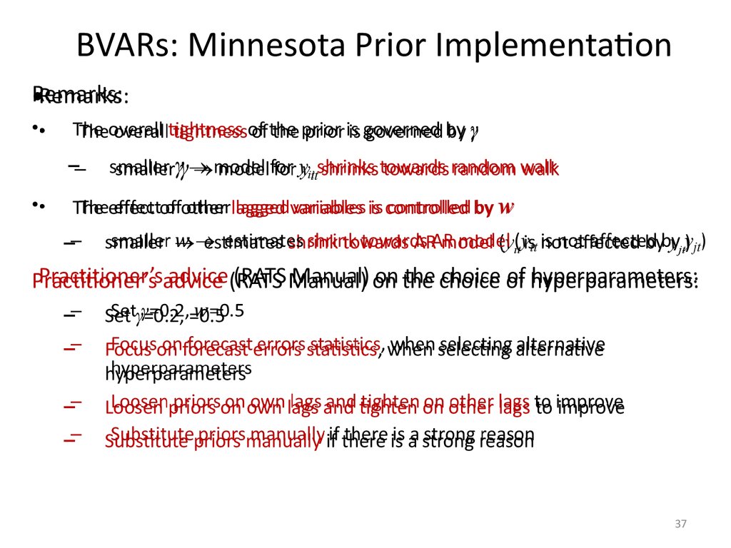
BVARs: Minnesota Prior ImplementationRemarks:
The overall tightness of the prior is governed by γ
–
smaller γ model for yit shrinks towards random walk
The effect of other lagged variables is controlled by w
–
smaller estimates shrink towards AR model (yit is not affected by yjt)
Practitioner’s advice (RATS Manual) on the choice of hyperparameters:
–
Set γ=0.2, =0.5
–
Focus on forecast errors statistics, when selecting alternative
hyperparameters
–
Loosen priors on own lags and tighten on other lags to improve
–
Substitute priors manually if there is a strong reason
37
38. BVARs: Prior Selection
Minnesota and conjugate priors are useful (e.g., to obtain
closed-form solutions), but can be too restrictive:
–
Independence across equations
–
Symmetry in the prior can sometimes be a problem
Increased computer power allows to simulate more general
prior distributions using numerical methods
Three examples:
–
DSGE-VAR approach: Del Negro and Schorfheide (IER, 2004)
–
Explore different prior distributions and hyperparameters: Kadiyala and
Karlsson (1997)
–
Choosing the hyperparameters to maximize the marginal likelihood:
Giannone, Lenza and Primiceri (2011)
38
39. Del Negro and Schorfheide (2004): DSGE-VAR Approach
Del Negro and Schorfheide (2004)
We want to estimate a BVAR model
We also have a DSGE model for the same variables
–
It can be solved and linearized: approximated with a RF VAR
–
Then, we can use coefficients from the DSGE-based VAR as prior means to
estimate the BVAR
• Several advantages:
–
DSGE-VAR may improve forecasts by restricting parameter values
–
At the same time, can improve empirical performance of DSGE relaxing its
restrictions
–
Our priors (from DSGE) are based on deep structural parameters consistent
with economic theory
39
40. Del Negro and Schorfheide (2004)
We estimate the following BVAR:
Y XA E
The solution for the DSGE model has a reduced-form VAR
representation
Y XA( ) U
where θ are deep structural parameters
Idea:
–
–
Combine artificial and T actual observations (Y,X) and to get the posterior
distribution
T*=λT “artificial” observations are generated from the DSGE model: (Y*,X*)
DSGE
Data
BVAR
40
41. Del Negro and Schorfheide (2004)
• Parameter λ is a “weight” of “artificial” (prior) data from DSGE–
λ=0 delivers OLS-estimated VAR: i.e. DSGE not important
–
Large λ shrinks coefficients towards the DSGE solution: i.e. data not
important
–
to find an “optimal” λ marginal likelihood is maximized (appendix E)
Can implement the procedure analytically… let’s see
41
42. Likelihood of the VAR of a DSGE Model
Recall the likelihood function for an unconstrained VAR
1
p (Y | A, ) | | T / 2 exp tr[ 1 (Y XA)' (Y XA)]
2
Similarly, the (Quasi-) likelihood for the “artificial” data:
1
p(Y * ( ) | A, e ) | e | T / 2 exp{ tr{ e 1[Y * ( ) X * ( ) A( )]'[Y * ( ) X * ( ) A( )]}
2
which is a prior density for the BVAR parameters
Rewrite the likelihood for the “artificial” data (open brackets)
p(Y * ( ) | A, e )
1
| e | T / 2 exp{ tr{ e 1[Y * ( )'Y * ( ) A( )' X * ( )'Y * ( ) Y * ( )' X * ( ) A( ) A( )' X * ( )' X * ( ) A( )]}
2
Sample moments
42
43. Likelihood of the VAR of a DSGE Model
Next step: we simulate s artificial observations (Y*,X*) from
the DSGE
…and replace sample moments like X ( )'Y ( ) with population
moments consistent with the DSGE model, e.g. :
*
*
1
lim X * ( )'Y * ( ) YX* ( )
s
s
The likelihood is then
p( A, e | )
1
*
{C ( )} 1 | e | ( T n 1) / 2 exp{ tr{ T e 1[ YY* ( ) A( )' XY* ( ) YX* ( ) A( ) A( )' XX
( ) A( )]}
2
where c(Θ) is chosen to ensure that the probability distribution integrates to one
(proper prior)
Population moments
43
44. DSGE-VAR prior
Conditional on the parameters , the DSGE m+odel provides a
conjugate priors for the BVAR
*
A | , e ~ N ( A* ( ), e ( T XX
( )) 1 )
e | ~ IWn ( T *e ( ), T k )
where parameters for prior distributions are maximum likelihood estimators
A* ( ) { YX* ( )} 1 YX* ( )
*
*e ( ) YY* ( ) YX* ( ){ YX* ( )} 1 XY
( )
For the conjugate priors we can obtain posteriors for A ande e
(conditional on ) of the same distribution family
44
45. DSGE-VAR posterior
Posterior, conditional on :
*
A | Y , , e ~ N ( Apos ( ), e [ T XX
( ) X ' X ] 1 )
e | Y , ~ IWn ((1 )T e , pos ( ), (1 )T k )
where
Prior info, weighted by λT
*
*
Apos ( ) [ T XX
( ) X ' X ] 1[ T XX
( ) X 'Y ]
Information from Data
e , pos ( )
1
[( T YX* ( ) Y ' X ) ...
(1 )T
*
*
... ( T YX* ( ) Y ' X )( T XX
( ) X ' X ) 1 ( T XY
( ) X 'Y )]
45
46. Results
BVARs (under different λ’s) have advantage in forecasting
performance (RMSE) vis-à-vis the unrestricted VAR
The “optimal” λ is about 0.6. It also delivers the best ex-post
forecasting performance for 1 quarter horizon
46
47. Results
BVAR with the DSGE prior under the “optimal” λ has better
forecasting performance than:
the unrestricted VAR for all variables
The BVAR with Minnesota Prior (ex. FF-rate at the shorter forecasting
horizon)
47
48. Kadiyala and Karlsson (1997)
Small Model: a bivariate VAR with unemployment and industrial
production
–
Sample period: 1964:1 to 1990:4.
–
Estimate the model through 1978:4
–
Criterion to chose hyperparameters: forecasting performance over 1979:1-1982:3
–
Use the remaining sub-sample 1982:4-1990:4 for forecasting
Large “”Litterman” Model: a VAR with 7 variables (real GNP, inflation,
unemployment, money, investment, interest rate and inventories)
–
Sample period: 1948:1 to 1986:4.
–
Estimate the model through 1980:1
–
Use the remaining sub-sample 1980:2-1986:4 for forecasting
48
49. Kadiyala and Karlsson (1997)
Compare different priors based on the VAR forecasting
performance (RMSE)
Standard VAR(p)…
yt A1 yt 1 ... Ap yt p et ,
E{et et' } e
… can be rewritten (see slide 29):
… and
Y XA E
y ( I n X ) e
where
E{e e'} e IT
e ~ N (0, e IT )
y vec(Y ), vec( A), e vec( E )
49
50. Prior distributions in K&K
Prior distributions in K&K• K&K use a number of competing prior distributions…
– Minnesota, Normal-Wishart, Normal-Diffuse, Extended Natural Conjugate
(see appendix E)
• … for and e
• Parameters of the prior distribution for :
–
each yit is a random walk (just as in Minnesota priors above)
yit yit 1 it
–
The variance of each coefficient depends on two hyper-parameters w, :
ï p , for coefficients of own lags
ï
Var ( i )
2
ï w ˆ i , for coefficients on lags of variables j i
ï p ˆ 2j
50
51. Prior distributions in K&K
Prior distributions in K&K• In the Small Model:
For prior distributions, hyper-parameters π1= , π2=w are selected based
on the forecast RMSEs over 1979:1-1982:3
(π1,π2) are fixed at the selected values and used in the forecasting exercise
over 1982:4-1990:4
51
52. Forecast Comparison in K&K: Small Model, unemployment
Forecast Comparison in K&K: Small Model,unemployment
Forecasting performance is
markedly different for different
priors
Normal-Wishart, Diffuse and
OLS do well (RMSEs are twice
lower than for other priors)
52
53. Forecast Comparison in K&K: Large Model
Forecast Comparison in K&K: Large Model• In the Large Model: hyper-parameters are fixed like in Litterman (1986)
OLS and Diffuse priors produce worst
forecasts in all cases
Normal-Wishart, Normal-Diffuse and
Minnesota do better (RMSEs are
substantially lower)
Lessons:
It does make sense to move from OLSestimated (over-parametrized VAR) to BVAR in
“Larger” model
Some prior distributions may lead to a
dominant forecasting performance
53
54. Giannone, Lenza and Primiceri (2011)
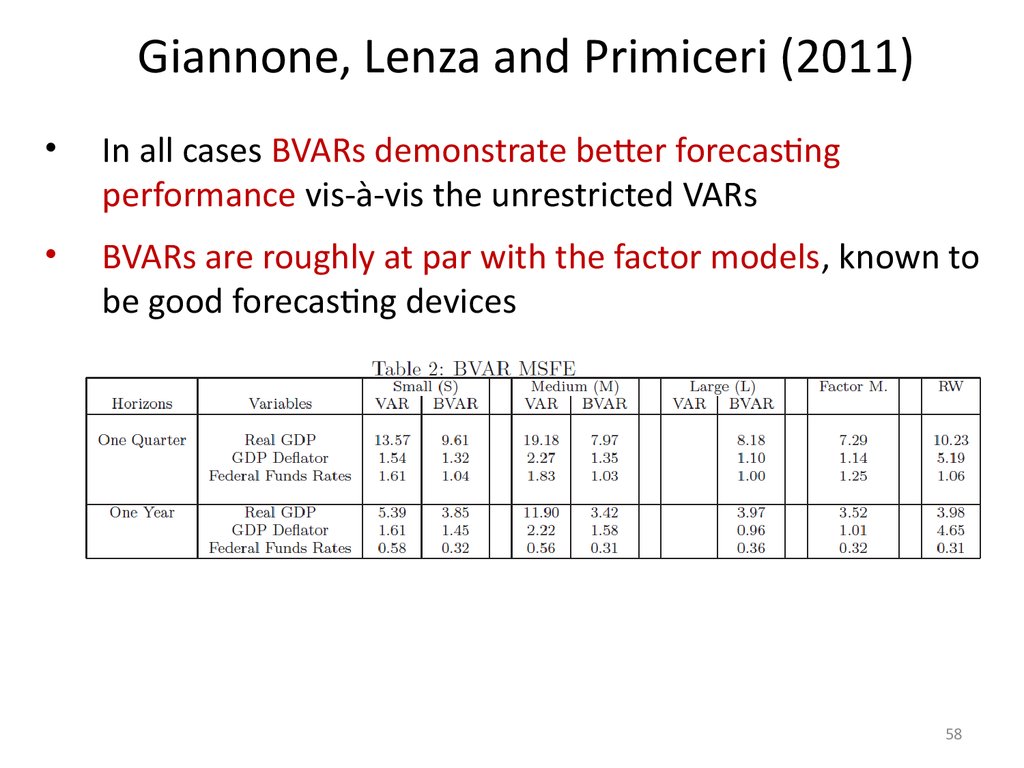
Use three VARs to compare forecasting performance
– Small VAR: GDP, GDP deflator, Federal Funds rate for the U.S
– Medium VAR: includes small VAR plus consumption, investment, hours
worked and wages
– Large VAR: expand the medium VAR with up to 22 variables
The prior distributions of the VAR parameters ϴ={ , Σ , Σe} depend
on a small number of hyperparameters
The hyperparameters are themselves uncertain and follow either
gamma or inverse gamma distributions
–
This is to the contrast of Minnesota priors where hyperparameters are
fixed!
54
55. Giannone, Lenza and Primiceri (2011)
The marginal likelihood is obtained by integrating
out the parameters of the model:
f ( y)
f ( y | )d f ( y | ) p ( )d
But the prior distribution of is itself a function of
the hyperparameters of the model i.e. p(θ)=p (θ|γ)
55
56. Giannone, Lenza and Primiceri (2011)
We interpret the model as a hierarchical model by replacing
pγ(θ)=p(θ|γ) and evaluate the marginal likelihood:
f ({ yt } | )
f ({ y }, ) p ( | )d
t
The hyperparameters γ are uncertain
Informativeness of their prior distribution is chosen via maximizing
the posterior distribution
p ( | y ) p ( y | ) p ( y )
Maximizing the posterior of γ corresponds to maximizing the onestep ahead forecasting accuracy of the model
56
57. Giannone, Lenza and Primiceri (2011)
5758.
Giannone, Lenza and Primiceri (2011)In all cases BVARs demonstrate better forecasting
performance vis-à-vis the unrestricted VARs
BVARs are roughly at par with the factor models, known to
be good forecasting devices
58
59. Conclusions
BVARs is a useful tool to improve forecasts
This is not a “black box”
–
posterior distribution parameters are typically functions of prior
parameters and data
Choice of priors can go:
–
from a simple Minnesota prior (that is convenient for analytical results)
–
…to a full-fledged DSGE model that incorporates theory-consistent
structural parameters
The choice of hyperparameters for the prior depends on the
nature of the time series we want to forecast
–
No “one size fits all approach”
59
60.
Thank You!60
61. Appendix A: Remarks about the marginal likelihood
Remarks about the marginal likelihood:
– If we have M1,….MN competing models, the marginal
likelihood of model Mj, f({yt}|Mj) can be seen as:
1.
2.
–
The update on the weight of model M j after observing the data
The out-of-sample prediction record of model j.
Model comparison between two models is performed
with the posterior odds ratio:
P(M1 |{yt}) P(M1 ) f ({ y }|M1 )
P(M2 |{ yt}) P(M2 ) f ({ y }|M2 )
–
Favor’s parsimonious modeling: in-built “Occam’s Razor.”
61
62. Appendix A: Remarks about the marginal likelihood
Remarks about the marginal likelihood:
–
–
Predict the first observation using the prior: f (y1 ) p( )L(y1 | )d
o
Record the first observable
p( )L(y1 |and
) its probability, f(y1 ). Update your
o
beliefs: p( | y1 )
f (y o )
1
– Predict the second observation:
Record f(y2o|y1o).
–
f (y2 | y1o ) p( | y1o )L(y2 | , y1o )d
Eventually, you get f({yo})=f(y1o) f(y2o|y1o)…..f(yTo|y1o, y2o,…, yT-1o).
62
63. Appendix B: Linear Regression with conjugate priors
• To calculate the posterior distribution for parametersf ( , 2 | y, X ) f ( y | X , , 2 ) f ( | 2 ) f ( 2 )
• …we assume the following for distributions:
– Normal for data
f ( y | X , , ) ( )
2
2
T
2
exp{
1
2 2
( y X )' ( y X )}
– Normal for the prior for β (conditional on σ2): β|σ2 ̴ N(m, σ2M)
k
2
f ( | ) ( ) exp{
2
2
1
( m)' M 1 ( m)}
2
2
– and Inverse-gamma for the prior for σ2 : σ2 ̴ IΓ(λ,k)
k
2
f ( ) ( ) exp{
2
2
}
2
2
• Next consider the product
f ( y | X , , 2 ) f ( | 2 )
63
64.
Appendix B: Linear Regression with conjugate priors• Rearranging the expressions under the exponents we have the
following:
( y X )' ( y X ) ( m)' M 1 ( m) ...
... ( y X ˆ )' ( y X ˆ ) ( ˆ )' X ' X ( ˆ ) ( m)' M 1 ( m) ...
... ( m* )' ( X ' X M 1 )( m* ) y ' y m* ' ( X ' X M 1 ) m* m' M 1m
where
ˆ ( X ' X ) 1 X ' y
is an OLS estimator of
m* ( X ' X M 1 ) 1 ( X ' X ˆ M 1m)}
Further denote
M * ( X ' X M 1 ) 1 ( X ' X M 1 ) ( M * ) 1
… and rewrite the
f ( , 2 | X , y )
1
( m* )' ( M * ) 1 ( m* )}
2
2
N T
1
y ' y m* ' ( M * ) 1 m* m' M 1m
2
2
( )
exp{
}
2 2
k
2
( ) exp{
2
65
65.
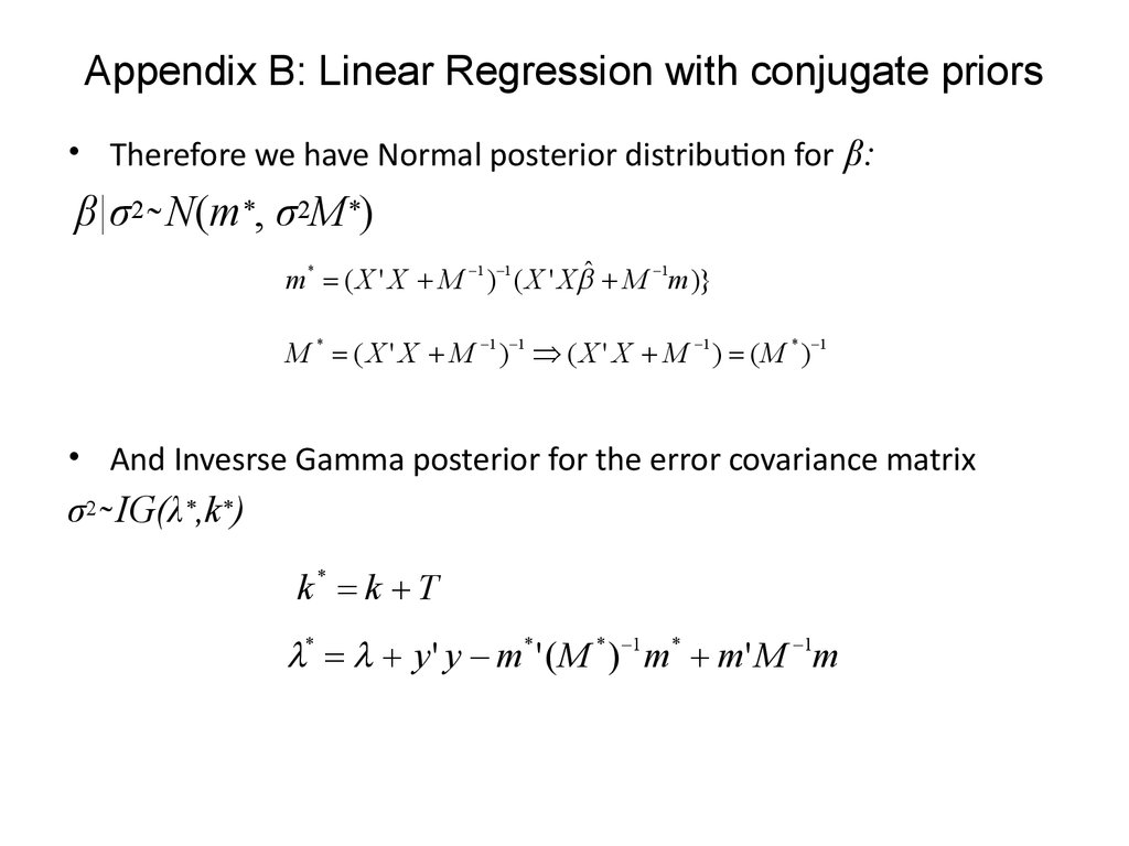
Appendix B: Linear Regression with conjugate priors• Therefore we have Normal posterior distribution for β:
β|σ2 ̴ N(m*, σ2M*)
m* ( X ' X M 1 ) 1 ( X ' X ˆ M 1m)}
M * ( X ' X M 1 ) 1 ( X ' X M 1 ) ( M * ) 1
• And Invesrse Gamma posterior for the error covariance matrix
σ2 ̴ IG(λ*,k*)
k* k T
* y ' y m* ' ( M * ) 1 m* m' M 1m
66. Appendix C: How to Estimate a BVAR, Case 1 prior
Use GLS estimator for the regression
y * X * e* , where
y * ,
y
I Ik
X* n
,
I
X
n
1
E{e*e* '}
0
0
e IT
1
0 * 1 *
0 *
GLS { X * '
X
}
{
X
'
y } ...
0 e IT
0 e IT
0
... {[ I n I k , ( I n X )' ]
0 e IT
1
0
I n I k 1
}
{[
I
I
,
(
I
X
)'
]
n
k
n
y } ...
I X
n
0 e IT
1
0
I n I k 1
}
{[
I
I
,
(
I
X
)'
]
n
k
n
y } ...
I X
n
0 e IT
0
... { [ I n I k , ( I n X )' ]
0 e IT
1
1
Continue (next slide)
66
67. Appendix C: How to Estimate a BVAR, Case 1 Prior
Continue
I n I k 1
1
1
... { [( I n I k ) , ( I n X )' ( e IT ) ]
} {( I n I k ) , ( I n X )' ( e IT ) } ...
y
In X
... { [( I n I k ) 1 ( I n I k ) ( I n X )' ( e IT ) 1 ( I n X )]} 1{( I n I k ) 1 ( I n X )' ( e I T ) 1 y} ...
1
1
.. note that I n I k I nk ,
( I n X )' ( e IT ) 1 ( I n X ) ( e 1 X ' )( I n X ) e 1 X ' X ,
( I n X )' ( e IT ) 1 ( e 1 X )' ...
... ( 1 e 1 X ' X ) 1 ( 1 ( e 1 X )' y )
So, the moments for the posterior distribution are:
* [ 1 e 1 ( X ' X )] 1 ( 1 e 1 X ' y )
Var ( * ) [ 1 e 1 ( X ' X )] 1 *
The posterior distribution is then multivariate normal
~ N ( * , * )
67
68. Appendix D: How to Estimate a BVAR: Conjugate Priors
• Note that in the case of the Conjugate priors we rely on the followingVAR representation
Y XA E
• … while in the Minnesota priors case we employed
y ( I n X ) e
• Though, if we have priors for vectorized coefficients in the form
~ N ( , )
• we can also get priors for coefficients
A ~ N ( A ,in Athe
) matrix form
• For the mean we simply Aneed to convert α back to the matrix form
A
• The variance
for... :
variance
for ... can
be
the
matrix
obtained from
2
c1
c c
a E{ '} c a
...
c b
1 2
1 11
1 22
c1c2
c2
c a
...
c b
2
2 11
2 22
a11c1
a c
a2
...
a b
11 2
11
11 22
b22 c1
... b c
... b a
...
... b2
22 2
22 11
22
2
c1
c a
A E{ A A '}
c b
1 11
1 12
2
c2
c a
2 21
...
...
c b
2 22
c1a11
c2 a21
a2 a2
...
...
a b a b
11
11 12
21
21 22
c1b12
c2b22
... a b a b
11 12
21 22
...
...
...
...
b2 b2
12
22
68
69. Appendix E: Prior and Posterior distributions in Kadiyala and Karlsson (1997)
6970. Appendix E: Posterior distributions of forecast for unemployment and industrial production in K&K (1997), h=4, T0 =1985:4
Appendix E: Posterior distributions of forecast forunemployment and industrial production in K&K (1997), h=4,
T0 =1985:4
70
71. Appendix E: Posterior distribution of the unemployment rate forecast in K&K (1997)
Appendix E: Posterior distribution of theunemployment rate forecast in K&K (1997)
71
72. Appendix E: Choosing λ
• Choosing in order to maximize the “empirical performance”of the DSGE-VAR
• Use the marginal data density:
p ( Y ) p ( Y | ) p( )d
• This can be interpreted as posterior probabilities for
• High posterior for large values of indicates that a lot of
weight should be placed in the DSGE model
• High posterior for low values of indicates information
about the degree of misspecification of the DSGE model
• Choose :
ˆ argmax p ( Y )
L
72