


")


")


 shock")
 shock")
 shock")


, “Factor Models for Macroeconomics,\" in J. B. Taylor and H. Uhlig (eds), Handbook of Macroeconomics, Vol. 2, North Holland.")


")


 economics
 english
Similar presentations:


Basics of factor models
1.
An Introduction to Factor ModellingJoint Vienna Institute / IMF ICD
Macro-econometric Forecasting and Analysis
JV16.12, L05, Vienna, Austria, May 19, 2016
Presenters
Massimiliano Marcellino
(Bocconi University)
Sam Ouliaris
This training material is the property of the International Monetary Fund (IMF) and is intended for use
in IMF Institute courses. Any reuse requires the permission of the IMF Institute.
2. Why factor models?
Appendix A: Details on estimation of factor modelsAppendix B: Details on Monte Carlocomparison
Why factor models?
● Factor models decompose the behaviour of an economic
variable (xit ) into a component driven by few unobservable
factors (f t ), common to all the variables but with specific
e"ects on them (λ i ), and a variable specific idiosyncratic
components (ξ i t ):
xit = li f t + xit ,
t = 1, ¼, T ; i = 1,..., N
● Idea of few common forces driving all economic variables is
appealing from an economic point of view, e.g. in the Real
Business Cycle (RBC) and Dynamic Stochastic Genereal
Equilibrium (DSGE) literature there are just a few key
economic shocks a"ecting all variables (productivity, demand,
supply, etc.), with additional variable specific shocks
● Moreover, factor models can handle large datasets (N large),
reflecting the use of large information sets by policy makers
and economic agents when taking their decisions
3. Why factor models?
Appendix A: Details on estimation of factor modelsAppendix B: Details on Monte Carlocomparison
Why factor models?
From an econometric point of view, factor models:
● Alleviate the curse of dimensionality of standard VARs
(number of parameters growing with the square of the number
of variables)
● Prevent omitted variable bias and issues of
non-fundamentalness of shocks (shocks depending on future
rather than past information that cannot be properly
recovered from VARs)
● Provide some robustness in the presence of structural
breaks
● Require minimal conditions on the errors (can be correlated
over time, heteroskedastic etc)
● Are relatively easy to be implemented (though underlying
model is nonlinear and with unobservable variables)
4. What can be done with factor models?
Appendix A: Details on estimation of factor modelsAppendix B: Details on Monte Carlocomparison
What can be done with factor models?
● Use the estimated factors to summarize the information in a
large set of indicators. For example, construct coincident and
leading indicators as the common factors extracted from a set
of coincident and leading variables, or in the same way
construct financial condition indexes or measures of global
inflation or growth.
● Use the estimated factors for nowcasting and forecasting,
possibly in combination with autoregressive (AR) terms
and/or other selected variables, or for estimation of missing or
outlying observations (getting a balanced dataset from an
unbalanced one). Typically, they work rather well.
● Identify the structural shocks driving the factors and their
dynamic impact on a large set of economic and financial
indicators (impulse response functions and forecast error
variance decompositions, as in structural VARs)
5. An introduction to factor models
Appendix A: Details on estimation of factor modelsAppendix B: Details on Monte Carlocomparison
An introduction to factor models
In this lecture we will consider:
● Small scale factor models: representation, estimation and
issues
● Large scale factor models
● Representation (exact/approximate, static/dynamic,
parametric / non parametric)
● Estimation: principal components, dynamic principal
components, maximum likelihood via Kalman filter, subspace
algorithms
● Selection of the number of factors (informal methods and
information criteria)
● Forecasting (direct / iterated)
● Structural analysis (FAVAR based)
● Useful references (surveys): Bai and Ng (2008), Stock and
Watson (2006, 2011, 2015), Lutekpohl (2014)
6. Some extensions
Appendix A: Details on estimation of factor modelsAppendix B: Details on Monte Carlocomparison
Some extensions
In the next lecture we will consider some relevant extensions for
empirical applications:
● How to allow for parameter time variation
● How to handle I(1) variables: Factor augmented Error
Correction Models
● How to handle hierarchical structures (e.g.,
countries/regions/sectors)
● How to handle nonlinearities
● How to construct targeted factors
● How to handle unbalanced datasets: missing observations,
mixed frequencies and ragged edges
7.
Appendix A: Details on estimation of factor modelsAppendix B: Details on Monte Carlocomparison
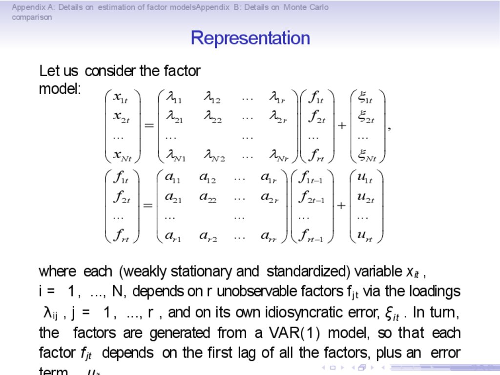
Representation
Let us consider the factor
model:
l
æ x ö æl
1t
11
12
ç
÷ ç
ç x2t ÷ = ç l21 l22
ç ... ÷ ç ...
ç
÷ ç
è xNt ø è lN 1 lN 2
æ f1t ö æ a11 a12
ç f ÷ ç
ç 2 t ÷ = ç a21 a22
ç ... ÷ ç ...
ç
÷ ç
è f rt ø è ar1 ar 2
...
...
...
l1r ö æ f1t ö æ x1t ö
l2 r ÷÷ çç f 2 t ÷÷ çç x 2 t ÷÷
+
,
÷ ç ... ÷ ç ... ÷
֍
÷ ç
÷
... lNr ø è f rt ø è x Nt ø
... a1r ö æ f1t -1 ö æ u1t ö
֍
÷ ç
÷
... a2 r ÷ ç f 2t -1 ÷ ç u2 t ÷
+
÷ ç ... ÷ ç ... ÷
...
֍
÷ ç
÷
... arr ø è f rt -1 ø è urt ø
where each (weakly stationary and standardized) variable xit ,
i = 1 , ..., N, depends on r unobservable factors f jt via the loadings
λ ij , j = 1 , ..., r , and on its own idiosyncratic error, ξ i t . In turn,
the factors are generated from a VAR(1) model, so that each
factor f j t depends on the first lag of all the factors, plus an error
8.
Appendix A: Details on estimation of factor modelsAppendix B: Details on Monte Carlocomparison
Representation
For example, xit , i = 1 , ..., N, t = 1 , ..., T can be:
● A set of macroeconomic and/or financial indicators for a
country →the factors represent their common drivers
● GDP growth or inflation for a large set of countries the
factors capture global movements in these two variables
● All the subcomponents of a price index → the factors capture
the extent of commonality among them and can be compared
with the aggregate index
● A set of interest rates of different maturities → commonality
is driven by level, slope and curvature factors
In general, we are assuming that all the variables are driven by a
(small) set of common unobservable factors, plus variable specific
errors.
9.
Appendix A: Details on estimation of factor modelsAppendix B: Details on Monte Carlocomparison
Let us write the factor model more compactly as:
Xt
=
Λ f t + ξt ,
ft
X t = ( x1t ,., xN t )'
-
ft = ( f1t ,..., f rt )'
L = (l ¢ ,., lN¢ )¢
where: 1
li = (li1 ,., lir )
under analysis
-
-
xt = (x1t ,., x Nt )
ut = (u1t ,..., urt )'
xt
ut
=
Af t—1 + ut ,
is the N x 1 vector of stationary variables
¢
is the r x 1 vector of unobservable factors
is the N x r matrix of loadings with
(measure effects of factors on variables)
is the N x 1 vector of idiosyncratic shocks
| lmax ( A) |< 1, | lmin ( A) |> 0
is the r x 1 vector of shocks to the factors
10.
Appendix A: Details on estimation of factor modelsAppendix B: Details on Monte Carlocomparison
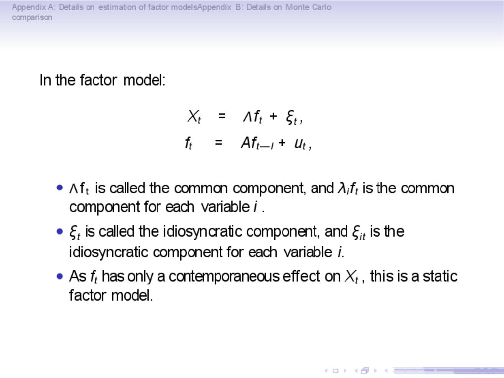
In the factor model:
Xt
=
Λ f t + ξt ,
ft
=
Af t—l + ut ,
● Λ f t is called the common component, and λ i f t is the common
component for each variable i .
● ξ t is called the idiosyncratic component, and ξ i t is the
idiosyncratic component for each variable i.
● As f t has only a contemporaneous effect on Xt , this is a static
factor model.
11.
Appendix A: Details on estimation of factor modelsAppendix B: Details on Monte Carlocomparison
● Additional lags of f t in the Xt equations can be easily allowed,
and we obtain a dynamic factor model. Additional lags in the
f t equations can be also easily allowed, as well as deterministic
components.
● If the variance covariance matrix of ξ t is diagonal (no
correlation at all among the idiosyncratic components), we
have a strict factor model. Otherwise, an approximate factor
model.
● As we have specified a model for the factors (VAR(1)), and
made specific assumption on the error structure (multivariate
white noise), we have a parametric factor model.
12.
Appendix A: Details on estimation of factor modelsAppendix B: Details on Monte Carlocomparison
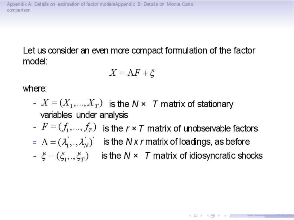
Let us consider an even more compact formulation of the factor
model:
X = LF + x
where:
- X = ( X 1 ,..., X T ) is the N × T matrix of stationary
variables under analysis
- F = ( f1 ,..., fT ) is the r × T matrix of unobservable factors
¢
¢ ¢
- L = (l1 ,., lN ) is the N x r matrix of loadings, as before
- x = (x1 ,., xT )
is the N × T matrix of idiosyncratic shocks
13. Identification
Appendix A: Details on estimation of factor modelsAppendix B: Details on Monte Carlocomparison
Identification
● Let us now consider two factor models:
X = LF + x , and
X = LP -1 PF + x = QG + x
where P is an r × r invertible matrix, Θ = ΛP — 1 and
G = PF .
● The two models for X are obervationally equivalent (same
likelihood), hence to uniquely identify the factors and the
loadings we need to impose a priori restrictions on Λ and/or
F.
● This is similar to the error correction model where the
cointegrating vectors and/or their loadings are properly
restricted to achieve identification.
14.
Appendix A: Details on estimation of factor modelsAppendix B: Details on Monte Carlocomparison
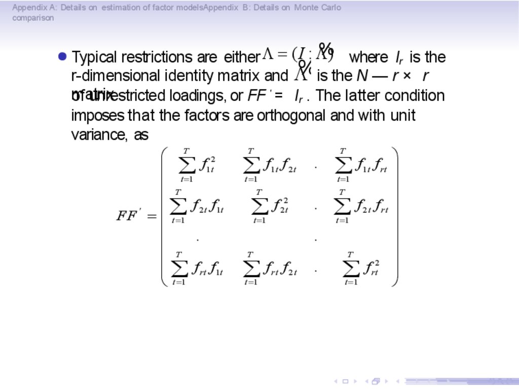
● Typical restrictions are either L
%) where l is the
= (I : L
r
%is the N — r × r
r-dimensional identity matrix and L
'
matrix
of unrestricted loadings, or FF = lr . The latter condition
imposes that the factors are orthogonal and with unit
variance, as
æ T
2
ç å f1t
t =1
ç
ç T
åf f
¢
FF = çç t =1 2t 1t
ç
.
ç T
ç
ç å f rt f1t
è t =1
T
t =1
1t
T
åf
t =1
f 2t
2
2t
.
.
.
T
åf
t =1
ö
f rt ÷
t =1
÷
T
÷
f 2 t f rt ÷
å
t =1
÷
÷
÷
T
2 ÷
f
å
rt
÷
t =1
ø
T
åf
rt
f 2t
.
åf
1t
15.
Appendix A: Details on estimation of factor modelsAppendix B: Details on Monte Carlocomparison
● The condition FF ' = lr is sufficient to get unique estimators for
the factors, but not to fully identify the model. For that
additional conditions are needed, such as Λ t Λ is diagonal
with distinct, decreasing diagonal elements. See, e.g.,
Lutkepohl (2014) for details.
16. Factor models and VARs
Appendix A: Details on estimation of factor modelsAppendix B: Details on Monte Carlocomparison
Factor models and VARs
An interesting question:
● Is there a VAR that is equivalent to a factor model (in the
sense of having the same likelihood)?
Unfortunately, in general no, at least not a finite order VAR.
However, it is possible to impose restrictions on a VAR to make it
"similar" to a factor model.
17.
Appendix A: Details on estimation of factor modelsAppendix B: Details on Monte Carlocomparison
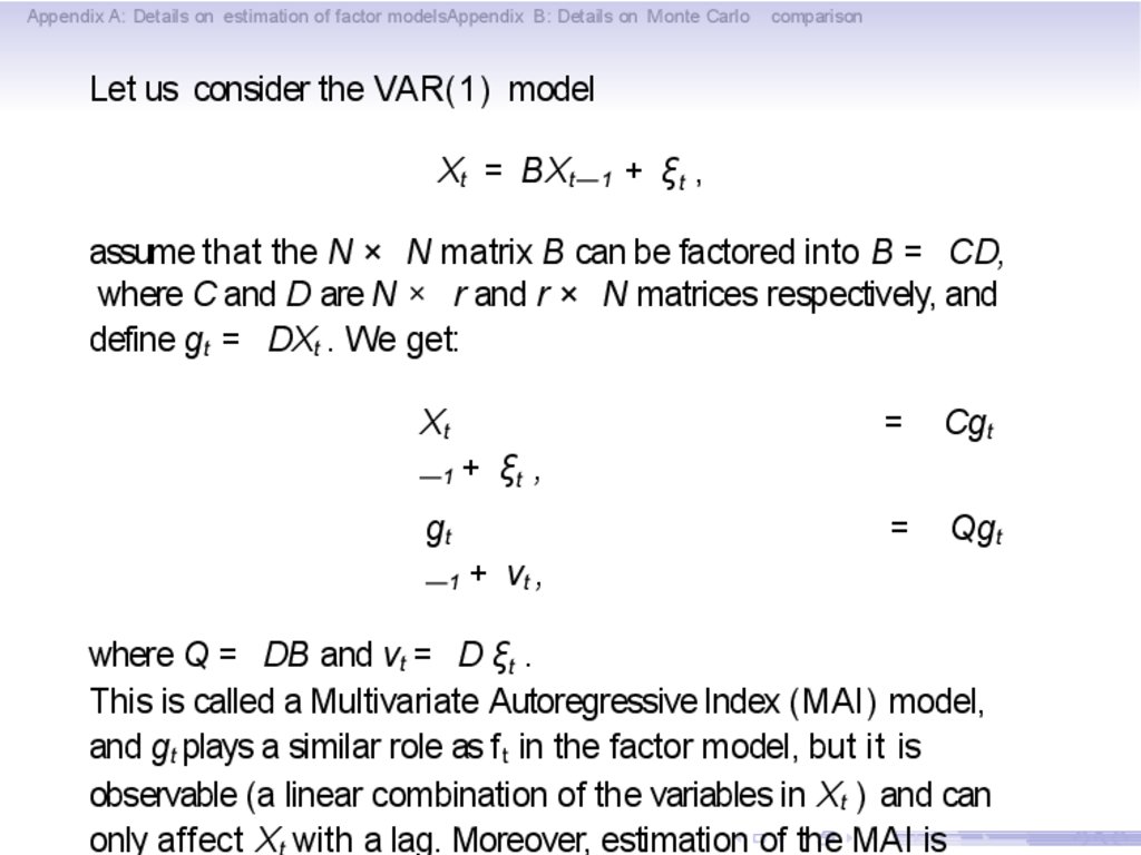
Let us consider the VAR(1) model
Xt = BX t—1 + ξ t ,
assume that the N × N matrix B can be factored into B = CD,
where C and D are N × r and r × N matrices respectively, and
define gt = DXt . We get:
Xt
—1
Cgt
=
Qgt
+ ξt ,
gt
—1
=
+ vt ,
where Q = DB and vt = D ξ t .
This is called a Multivariate Autoregressive Index (MAI) model,
and gt plays a similar role as f t in the factor model, but it is
observable (a linear combination of the variables in Xt ) and can
only affect X with a lag. Moreover, estimation of the MAI is
18. Estimation by the Kalman filter
Appendix A: Details on estimation of factor modelsAppendix B: Details on Monte Carlocomparison
Estimation by the Kalman filter
Let us consider again the factor model written as:
Xt
=
Λft
+
ξt ,
ft
ut .
=
Af t—1 +
In this formulation:
● the factors are unobservable states,
● Xt = Λ f t
+ ξ t are the observation equations (linking the
unobservable states to the observable variables),
● f t = Af t —1 + ut are the transition equations (governing the
evolution of the states).
19.
Appendix A: Details on estimation of factor modelsAppendix B: Details on Monte Carlocomparison
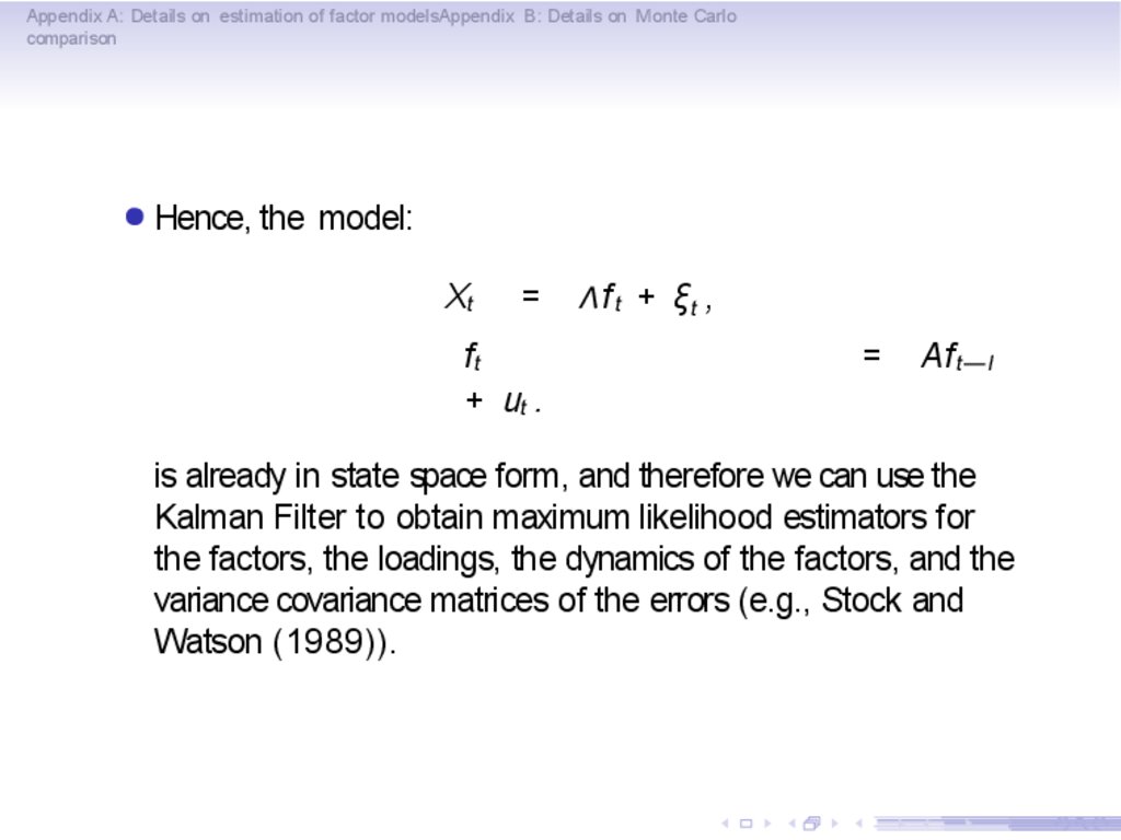
● Hence, the model:
Xt
=
ft
+ ut .
Λ f t + ξt ,
=
Af t—l
is already in state space form, and therefore we can use the
Kalman Filter to obtain maximum likelihood estimators for
the factors, the loadings, the dynamics of the factors, and the
variance covariance matrices of the errors (e.g., Stock and
Watson (1989)).
20.
Appendix A: Details on estimation of factor modelsAppendix B: Details on Monte Carlocomparison
However, there are a few problems:
● First, the method is computationally demanding, so that it is
traditionally considered applicable only when the number of
variables, N, is small.
● Second, with N finite, we cannot get consistent estimators for
the factors (as the latter are random variables, not
parameters).
● Finally, the approach requires to specify a model for the
factors, which can be difficult as the latter are not observable.
Hence, let us consider alternative estimation approaches.
21. Non-parametric, large N, factor models
Appendix A: Details on estimation of factor modelsAppendix B: Details on Monte Carlocomparison
Non-parametric, large N, factor models
● There are two competing approaches in the factor literature
that are non-parametric, allow for very large N (in theory
N →∞) and produce consistent estimators for the factors
and/or the common components. They were introduced by
Stock and Watson (2002a, 2002b, SW) and Forni, Hallin,
Lippi and Reichlin (2000, FHLR), and later refined and
extended in many other contributions, see e.g. Bai and Ng
(2008) for an overview.
● We will now review their main features and results, starting
with SW (which is simpler) and then moving to FHLR.
22. The SW approach - PCA
Appendix A: Details on estimation of factor modelsAppendix B: Details on Monte Carlocomparison
The SW approach - PCA
● The Stock and Watson (2002a,2002b) factor model is
Xt = Λ f t ‡ ξ t ,
where:
● Xt is N × 1 vector of stationary variables
● f t is r × 1 vector of common factors, can be correlated
over time
● Λ is N × r matrix of loadings
● ξ t is N × 1 vector of idiosyncratic disturbances, can be mildly
cross-sectionally and temporally correlated
● conditions on Λ and ξ t guarantee that the factors are
pervasive
(affect most variables) while idiosyncratic errors are not.
23. The SW approach - PCA
Appendix A: Details on estimation of factor modelsAppendix B: Details on Monte Carlocomparison
The SW approach - PCA
● Estimation of Λ and f t in the model Xt = Λ f t + ξ t is complex
because of nonlinearity (Λ f t ) and the fact that f t is a random
variable rather than a parameter.
● The minimization problem we want to solve is
T
min (Λå) (X t - Λft )' X t - f t
Λ, f1 , f 2 ,..., fT
t =1
● Under mild regularity conditions, it can be shown that the
(space spanned by the) factors can be consistently estimated
by the first r static principal components of X (PCA).
24. The SW approach - Choice of r
Appendix A: Details on estimation of factor modelsAppendix B: Details on Monte Carlocomparison
The SW approach - Choice of r
Choice of the number of factors, r :
● Fraction of explained variance of Xt : should be large (though
decreasing) for the first r principal components, very small for
the remaining ones
● Information criteria (Bai and Ng (2002): r should minize
properly defined information criteria (cannot use standard
ones as now not only T but also N can diverge)
● Testing: Kapetanios (2010) provides some statistics and
related distributions, not easy
25. The SW approach - Properties of PCA
Appendix A: Details on estimation of factor modelsAppendix B: Details on Monte Carlocomparison
The SW approach - Properties of PCA
● Need both N and T to grow large, and not too much cross-
correlation among idiosyncratic errors.
● As a basic example, consider case with one factor and
uncorrelated idiosyncratic errors (exact factor model):
(1)
xit = λ i f t + eit .
Then, use simple cross-sectional average as factor estimator:
1
N
æ1 N ö
1
x
=
x
=
t
å
it
ç N å li ÷ ft + N
i =1
è i =1 ø
lim x t = l f t
N
N
åe
it
i =1
N ®¥
And is consistent for x t (up to a scalar). We can also get
factor loadings by OLS regression of xit on x t and
l
lim lˆ i = i
T ®¥
l
So, if both N and T diverge lˆ i x t ® li f t .
26. The SW approach - Properties of PCA
Appendix A: Details on estimation of factor modelsAppendix B: Details on Monte Carlocomparison
The SW approach - Properties of PCA
● PCA are weighted rather than simple averages of the
variables, where weights depend on λ i and var(eit ).
● Under general conditions and with proper standardization,
PCA and estimated loadings have asymptotic Normal
distributions (Bai Ng (2006))
● If N grows faster than T (such that T 1 / 2 /N goes to zero),
the estimated factors can be treated as true factors when used
in second-step regressions (e.g. for forecasting, factor
augmented VARs, etc.). Namely, there are no generated
regressor problems.
● If the factor structure is weak (first factor explains little
percentage of overall variance), PCA is no longer consistent
(Onatski (2006)).
27. The SW approach - Properties of PCA based forecasts
Appendix A: Details on estimation of factor modelsAppendix B: Details on Monte Carlocomparison
The SW approach - Properties of PCA based forecasts
● Suppose the model is
Yt + 1
= ft β +
vt ,
Xt
+ ξt ,
=
Λft
then we can construct yˆat +1forecast
= fˆ t bˆ ,as
where fˆ t are the PCA factor estimators andbˆ the
OLS estimator of , obtained by regressing yt+1 on fˆ t .
• The asymptotic distribution of factor based forecasts is also
Normal, under general conditions, and its variance depends on the
variance of the loadings and on that of the factors, so you need both
and large to get a precise forecast (Bai and Ng (2006)). This results
can be used to derive interval and density factor based forecasts.
28. The FHLR approach - DPCA
Appendix A: Details on estimation of factor modelsAppendix B: Details on Monte Carlocomparison
The FHLR approach - DPCA
● The FHLR factor model is
Xt = B(L)u t + ξ t = χ t + ξ t ,
where:
● Xt is the N × 1 vector of stationary variables
● ut is the q × 1 vector of i.i.d. orthonormal common shocks.
These are the drivers of the common factors in the SW
formulation, but in FHLR the focus in on the common shocks
rather than the common factors)
● B(L) = 1 + B 1 L + B2 L2 + ... + Bp Lp
● χ t = B ( L ) u t is the N × 1 vector of common components. It
is estimated by Dynamic Principal Components (DPCA),
details in Appendix A.
● ξ t is the N × 1 vector of idiosyncratic shocks, can be mildly
correlated across units and over time
● Conditions on B(L) and ξ t guarantee that the factors are
29. The FHLR approach - static and dynamic factors
Appendix A: Details on estimation of factor modelsAppendix B: Details on Monte Carlocomparison
The FHLR approach - static and dynamic factors
● q can be different from r : the former is usually referred to as
the number of dynamic factors while r is the number of static
factors, with q ≤ r .
● Let us assume for simplicity that there is a single factor f t , but
it has both a contemporaneous and lagged effect on X t :
Xt
ξt ,
=
Λ 1 f t + Λ 2 ft — 1 +
We can define gtf t = (f', f' )' , Λ = ( Λ=1 , Λaf2 t—1
), and
+ uwrite
t.
t
t- l
model
in
static
form
the
as
Xt = Λg t + ξ t .
In this case we have r = 2 static factors (those in gt ), which
are all driven by q = 1 common shock (ut ). Typically, FHLR
focus on q (and the common shocks ut ), while SW on r (and
the common factors gt ). The distinction matters more for
structural analysis than for forecasting.
30. The FHLR approach - Choice of q
Appendix A: Details on estimation of factor modelsAppendix B: Details on Monte Carlocomparison
The FHLR approach - Choice of q
● Informal methods:
-Estimate recursively the spectral density matrix of a subset of
Xt , increasing the number of variables at each
the dynamic
eigenvalues for a grid of frequencies,lqx choose
step¡
calculate
q that when the number of variables increases the
so
average
over frequencies of the first q dynamic eigenvalues diverges,
while the average of the q + 1 t h does not.
-For the whole Xt there should be a big gap between the
variance of X t explained by the first q dynamic principal
components and that explained by the q + 1 t h
component.
● Formal methods:
-Information criteria: Hallin Liska (2007); Amengual and
Watson (2007)
31. The FHLR approach - Forecasting
Appendix A: Details on estimation of factor modelsAppendix B: Details on Monte Carlocomparison
The FHLR approach - Forecasting
● Consider now the model (direct estimation, the common
shocks have an h-period delay in effecting Xt ):
X t + h = B(L)u t + ξ t + h = χ t + ξ t + h .
In this context, an optimal linear forecast for Xt + h Is cˆ t
that can be obtained, as said, by
DPCA.
●A
problem with using this method for forecasting is the use of
future information in the computation of the DPCA. To
overcome this issue, which prevents a real time
implementation of the procedure, Forni, Hallin, Lippi and
Reichlin (2005) propose a modified one-sided estimator (which
is however too complex for implementation in EViews).
32. Parametric estimation - quasi MLE
Appendix A: Details on estimation of factor modelsAppendix B: Details on Monte Carlocomparison
Parametric estimation - quasi MLE
● Kalman filter produces (quasi-) ML estimators of the factors,
but considered not feasible for large N. No longer true: Doz,
Giannone, Reichlin (2011, 2012).
● Model has the form
Xt = Λ f t +
ξt ,
Ψ(L)f t = B
where q-dimensional vector ηt contains the orthogonal
ηt ,
dynamic shocks driving the r factors f t , and the matrix B is
(r × q)-dimensional, with q ≤ r .
● For given r and q, estimation proceeds in the following
steps:
(2)
(3)
33. Parametric estimation - quasi MLE
Appendix A: Details on estimation of factor modelsAppendix B: Details on Monte Carlocomparison
Parametric estimation - quasi MLE
34. Parametric estimation - Subspace algorithms (SSS)
Appendix A: Details on estimation of factor modelsAppendix B: Details on Monte Carlocomparison
Parametric estimation - Subspace algorithms (SSS)
● Let us now consider again the factor model:
Xt
=
Du
,
t
=
l
,
.
.
.
,
T
ft t =
Cft +
(4)
Af t-1 + Bu t-1
Kapetanios and Marcellino (2009, KM) show that (4) can be
written as regression of future on past, with particular reduced
rank restrictions on the coefficients (similar to reduced rank
VAR seen above):
(5)
X t f = OK X tp + EEt f
Where , f
'
'
'
p
'
'
X t = ( X t , X t +1 , X t + 2 ,...) ', X t = ( X t -1 , X t - 2 ,...),
Et = (ut' , ut' +1 ,...) '
f
p
f
• Note that (i) X t = OK X t + EEt and (ii) fˆt =p Kˆ X tp .
Hence, best linear predictor of future X isOKX t , and we need
ˆ ˆ p , ).
and estimator for K ( and for the loadings X t f = OKX
t
f
35. Parametric estimation - SSS
Appendix A: Details on estimation of factor modelsAppendix B: Details on Monte Carlocomparison
Parametric estimation - SSS
● KM show how to obtains the SSS factor estimates,
fˆt = Kˆ X tp .
See Appendix A for
● details.
Once estimates of the factors are available, estimates of the
other parameters (including the factor loadings, Oˆ ) can be
obtained by OLS.
● Choice of number of factors can be done by information
criteria, similar to those by Bai and Ng (2002) for PCA but
with different penalty function, see KM.
36. Parametric estimation - SSS forecasts
Appendix A: Details on estimation of factor modelsAppendix B: Details on Monte Carlocomparison
Parametric estimation - SSS forecasts
ˆ ˆ p , where Oˆ
X t f = OKX
t
is obtained
by
OLS regression on the estimated factors,
as in
● With
PCA. MLE forecasts are obtained by iterated method (VAR for
factors is iterated forward to produce forecasts for the factors,
which are then inserted into the static model for Xt ).
Forecasts obtained by PCA, DPCA and SSS use direct method
(variable of interest is regressed on the estimated factors
lagged h periods, and parameter estimates are combined with
current value of the estimated factors to produce h-step
ahead forecast of variable(s) of interest).
● If model is correctly specified, MLE plus iterated method
produces better (more efficient) forecasts. If there is
mis-specification, as it is often the case, the ranking is not
clear-cut, other factor estimation approaches plus direct
estimation can be better. See, e.g., Marcellino, Stock and
Watson (2006) for comparison of direct and iterated
forecasting with AR and VAR models.
● The SSS forecasts are
37. Factor estimation methods - Monte Carlo Comparison
Appendix A: Details on estimation of factor modelsAppendix B: Details on Monte Carlocomparison
Factor estimation methods - Monte Carlo Comparison
● Comparison of PCA, DPCA, MLE and SSS (based on
Kapetanios and Marcellino (2009, KM)).
● The DGP is:
xt = Cft + e t , t = 1,¼, T
A( L) ft = B ( L)ut
A( L) = I - A1 ( L) -¼- Ap ( L)
Where
B ( L) = I + B1 ( L) +¼+ Bq ( L)
,with (N,
(6)
T ) = (50,50),
(200,50).
MLE(100,50),
for (50,50)(100,100),
only, due to(50,500),
computational
(50,100),
burden.
(100,500)and
● Experiments differ for number of factors (one or several), A
and B matrices, choice of s (s = m or s = 1) , factor
loadings (static or dynamic), choice of number of factors
(true number or misspecified), properties of idiosyncratic
errors (uncorrelated or serially correlated), and the way C
matrix is generated (standard normal or uniform with non-zero
38. Factor estimation methods - MC Comparison, summary
Appendix A: Details on estimation of factor modelsAppendix B: Details on Monte Carlocomparison
Factor estimation methods - MC Comparison, summary
● Appendix B provides more details on the DGP and detailed
results. The main findings are the following:
● DPCA shows consistently lower correlation between true and
estimated common components than SSS and PCA. It shows,
in general, more evidence of serial correlation of idiosyncratic
components, although not to any significant extent.
● SSS beats PCA, but gains are rather small, in the range
5-10%, and require a careful choice of s.
● SSS beats MLE, which is only sligthly better than
PCA.
● All methods perform very well in recovering the common
components. As PCA is simpler, it seems reasonable to use
it.
39. Factor models - Forecasting performance
Appendix A: Details on estimation of factor modelsAppendix B: Details on Monte Carlocomparison
Factor models - Forecasting performance
● Really many papers on forecasting with factor models in the
past l5 years, starting with Stock and Watson (2002b) for the
USA and Marcellino, Stock and Watson (2003) for the euro
area. Banerjee, Marcellino and Masten (2006) provide results
for ten Eastern European countries. Eickmeier and Ziegler
(2008) provide nice summary (meta-analysis), see also Stock
and Watson (2006) for a survey of the earlier results.
● Recently used also for nowcasting, i.e., predicting current
economic conditions (before official data is released). More on
this in the next lecture.
40. Factor models - Forecasting performance
Appendix A: Details on estimation of factor modelsAppendix B: Details on Monte Carlocomparison
Factor models - Forecasting performance
Eickmeier and Ziegler (2008):
● "Our results suggest that factor models tend to outperform
small models, whereas factor forecasts are slightly worse than
pooled forecasts. Factor models deliver better predictions for
US variables than for UK variables, for US output than for
euro-area output and for euro-area inflation than for US infl
ation. The size of the dataset from which factors are
extracted positively affects the relative factor forecast
performance, whereas pre-selecting the variables included in
the dataset did not improve factor forecasts in the past.
Finally, the factor estimation technique may matter as
well."
41. Structural Factor Augmented VAR (FAVAR)
Appendix A: Details on estimation of factor modelsAppendix B: Details on Monte Carlocomparison
Structural Factor Augmented VAR (FAVAR)
● To illustrate the use of the FAVAR for structural analysis, we
take as starting point the FAVAR model as proposed by
Bernanke, Boivin and Eliasz (2005, BBE), see also Eickmeier,
Lemke and Marcellino (2015, ELM) for extensions and
Lutkepohl (2014), Stock and Watson (2015) for surveys.
● The model for a large set of stationary macroeconomic and
financial variables is:
(7)
x i,t = Λ 'i Ft + ei,t , i = 1 , . . .
N, are orthonormal (F 'F = l ) and uncorrelated
where the factors
with the idiosyncratic errors, and E (et ) = 0, E (et et') = R,
where R is a diagonal matrix. As we have seen, these
assumptions identify the model and are common in the FAVAR
literature.
● The dynamics of the factors are then modeled as a VAR(p),
Ft = B 1 F t — 1 + . . . Bp Ft—p +
wt ,
'
E (w t ) = 0, E (w t w
t ) =
(8)
W.
42. Structural FAVAR
Appendix A: Details on estimation of factor modelsAppendix B: Details on Monte Carlocomparison
Structural FAVAR
● The VAR equations in (8) can be interpreted as a
reduced-form representation of a system of the
form
PFt = K l F t — l + . . . K p Ft—p +
E (ut ) = 0, E (ut tu') =
(9)
S,
ut ,
where P is lower-triangular with ones on the main diagonal,
and S is a diagonal matrix.
● The relation to the reduced-form parameters in (8) is
Bi = P —1 K i and W = P—1 SP—1’ . This system of equations
is often referred to as a ‘structural VAR' (SVAR)
representation, obtained with Choleski identification.
● For the structural analysis, BBE assume that Xt is driven
by
G latent factors Ft* and the Federal Funds rate (i t ) as a
(G + 1) th observable factor, as they are interested in
measuring the effects of monetary policy shocks in the
economy. ELM use G = 5 factors, that provide a
43. Structural FAVAR - Monetary policy shock identification
Appendix A: Details on estimation of factor modelsAppendix B: Details on Monte Carlocomparison
Structural FAVAR - Monetary policy shock identification
● The space spanned by the factors can be estimated by PCA
using, as we have seen, the first G + 1 PCs of the data Xt
(BBE also consider other factor estimation methods).
● To remove the observable factor i t from the space spanned by
all G + 1 factors, dataset is split into slow-moving variables
(expected to move with delay after an interest rate shock),
and fast-moving variables (can move instantaneously).
Slow-moving variables comprise, e.g., real activity measures,
consumer and producer prices, deflators of GDP and its
components and wages, whereas fast-moving variables are
financial variables such as asset prices, interest rates or
commodity prices.
44. Structural FAVAR - Monetary policy shock identification
Appendix A: Details on estimation of factor modelsAppendix B: Details on Monte Carlocomparison
Structural FAVAR - Monetary policy shock identification
● In line with BBE, ELM estimate the first G PCs from the
set
of slow-moving variables, denoted by Fˆt slow .
● Then, they carry out a multiple regression of Ft
ˆ Fˆ t + eˆi ,t ,
on i t , i.e.
xi ,t = Λ'
i
Ft = a Fˆt slow t + bit +n t .
• An estimate of
Ft * is then given by aF
ˆ ˆt slow .
Fˆt slow and
45. Structural FAVAR - Monetary policy shock identification
Appendix A: Details on estimation of factor modelsAppendix B: Details on Monte Carlocomparison
Structural FAVAR - Monetary policy shock identification
● In the joint factor vectorFt
º [ Fˆt* , it ] the Federal Funds rate it
is ordered last. Given this ordering, the VAR representation
with lower-triangular contemporaneous-relation matrix P in
(8) directly identifies the monetary policy shock as the last
element of the innovation vector ut , say uint,t . Hence, the
shock identification works via a Cholesky decomposition,
which is here readily given by the lower triangular P — 1 .
● Naturally, the methodology also allows for other identification
approaches, such as short/long run or sign restrictions. These
*
can be just applied to the VAR for Ft º [ Fˆt , it ].
● Impulse responses of the factors to the monetary policy
shock,
∂F t+h /∂uint,t , are then computed inˆ theˆ usual fashion from
x = Λ'i F t + eˆi ,t ,
estimated
loading
equations,
the estimated
VAR,
and used ini ,t conjunction
with the
To get, ∂x i,t+ h /∂uint,t . Proper confidence bands for the
impulse response functions can be computed by using the
bootstrap method.
46. Structural FAVAR - Monetary policy (FFR) shock
Appendix A: Details on estimation of factor modelsAppendix B: Details on Monte Carlocomparison
Structural FAVAR - Monetary policy (FFR) shock
Impulse responses from constant parameter FAVAR (solid) and
time varying FAVAR (averages over all periods, dotted) for key
variables, taken from ELM (who developed the TV-FAVAR,
discussed in next lecture)
47. Structural FAVAR - Monetary policy (FFR) shock
Appendix A: Details on estimation of factor modelsAppendix B: Details on Monte Carlocomparison
Structural FAVAR - Monetary policy (FFR) shock
Impulse responses from FAVAR (solid) and TV-FAVAR (dotted)
48. Structural FAVAR - Monetary policy (FFR) shock
Appendix A: Details on estimation of factor modelsAppendix B: Details on Monte Carlocomparison
Structural FAVAR - Monetary policy (FFR) shock
Impulse responses from FAVAR (solid) and TV-FAVAR (dotted)
49. Structural FAVAR: Summary
Appendix A: Details on estimation of factor modelsAppendix B: Details on Monte Carlocomparison
Structural FAVAR: Summary
● Structural factor augmented VARs are a promising tool as
they address several issues with smaller scale VARs, such as
omitted variable bias, curse of dimensionality, possibility of
non-fundamental shocks, etc.
● FAVAR estimation and computation of the responses to
structural shocks is rather simple, though managing a large
dataset is not so simple
● Some problems in VAR analysis remain also in FAVARs, in
particular robustness to alternative identification schemes,
parameter instability, nonlinearities, etc.
● In the next lecture we will consider some extensions of the
basic model that will address some of these issues.
50. References
Appendix A: Details on estimation of factor modelsAppendix B: Details on Monte Carlocomparison
References
Amengual, D. and Watson, M.W. (2007), "Consistent
estimation of the number of dynamic factors in a large N and
T panel", Journal of Business and Economic Statistics, 25(l),
9l-96
Bai, J. and S. Ng (2002). "Determining the number of factors
in approximate factor models". Econometrica, 70, l9l-22l.
Bai, J. and Ng, S., (2006). "Confidence Intervals for Diffusion
Index Forecasts and Inference for Factor-Augmented
Regressions," Econometrica, 74(4), ll33-ll50.
Bai, J., and S. Ng (2008), “Large Dimensional Factor
Analysis,” Foundations and Trends in Econometrics, 3(2):
89-l63.
Bauer, D. (l998), Some Asymptotic Theory for the Estimation
of Linear Systems Using Maximum Likelihood Methods or
Subspace Algorithms, Ph.d. Thesis.
51.
Appendix A: Details on estimation of factor modelsAppendix B: Details on Monte Carlocomparison
Banerjee, A., Marcellino, M.and I. Masten (2006).
“Forecasting macroeconomic variables for the accession
countries”, in Artis, M., Banerjee, A. and Marcellino, M.
(eds.), The European Enlargement: Prospects and Challenges,
Cambridge: Cambridge University Press.
Bernanke, B.S., Boivin, J. and P. Eliasz (2005). "Measuring
the e"ects of monetary policy: a factor-augmented vector
autoregressive (favar) approach", The Quarterly Journal of
Economics, l20(l), 387–422.
Carriero, A., Kapetanios, G. and Marcellino, M. (20ll),
“Forecasting Large Datasets with Bayesian Reduced Rank
Multivariate Models”, Journal of Applied Econometrics, 26,
736-76l.
Carriero, A., Kapetanios, G. and Marcellino, M. (20l6),
"Structural Analysis with Classical and Bayesian Large
Reduced Rank VARs", Journal of Econometrics,
forthcoming.
52.
Appendix A: Details on estimation of factor modelsAppendix B: Details on Monte Carlocomparison
Doz, C., Giannone, D. and L. Reichlin (20ll). "A two-step
estimator for large approximate dynamic factor models based
on Kalman filtering," Journal of Econometrics, l64(l),
l88-205.
Doz, C., Giannone, D. and L. Reichlin (20l2). "A Quasi–
Maximum Likelihood Approach for Large, Approximate
Dynamic Factor Models," The Review of Economics and
Statistics, 94(4), l0l4-l024.
Eickmeier, S., W. Lemke, M. Marcellino, (20l4). "Classical
time-varying FAVAR models - estimation, forecasting and
structural analysis", Journal of the Royal Statistical Society,
forthcoming.
Eickmeier, S. and Ziegler, C. (2008). "How successful are
dynamic factor models at forecasting output and inflation? A
meta-analytic approach", Journal of Forecasting, (27),
237-265.
53.
Appendix A: Details on estimation of factor modelsAppendix B: Details on Monte Carlocomparison
Forni, M., Hallin, M., Lippi, M. and L. Reichlin (2000), “The
generalised factor model: identification and estimation”, The
Review of Economic and Statistics, 82, 540-554.
Forni, M., M. Hallin, M. Lippi, L. Reichlin (2005), "The
Generalized Dynamic Factor Model: One-sided estimation and
forecasting", Journal of the American Statistical Association,
l00, 830-840.
Hallin, M., and Liška, R., (2007), “The Generalized Dynamic
Factor Model: Determining the Number of Factors,” Journal
of the American Statistical Association, l02, 603-6l7
Kapetanios, G. (20l0), "A Testing Procedure for Determining
the Number of Factors in Approximate Factor Models With
Large Datasets". Journal of Business and Economic Statistics,
28(3), 397-409.
Kapetanios, G., Marcellino, M. (2009). "A parametric
estimation method for dynamic factor models of large
dimensions". Journal of Time Series Analysis 30, 208-238.
54.
Appendix A: Details on estimation of factor modelsAppendix B: Details on Monte Carlocomparison
Lutkepohl, H. (20l4), "Structural vector autoregressive
analysis in a data rich environment", DIW WP.
Marcellino, M., J.H. Stock and M.W. Watson (2003),
“Macroeconomic forecasting in the Euro area: country specific
versus euro wide information”, European Economic Review,
47, l-l8.
Marcellino, M., J. Stock and M.W. Watson, (2006), “A
Comparison of Direct and Iterated AR Methods for Forecasting
Macroeconomic Series h-Steps Ahead”, Journal of
Econometrics, l35, 499-526.
Onatski, A. (2006). "Asymptotic Distribution of the Principal
Components Estimator of Large Factor Models when Factors
are Relatively Weak". Mimeo.
Stock, J.H and M.W. Watson (l989), “New indexes of
coincident and leading economic indicators.” In NBER
Macroeconomics Annual, 35l–393, Blanchard, O. and S.
Fischer (eds). MIT Press, Cambridge, MA.
55.
Appendix A: Details on estimation of factor modelsAppendix B: Details on Monte Carlocomparison
Stock, J.H and M.W. Watson (2002a), “Forecasting using
Principal Components from a Large Number of Predictors”,
Journal of the American Statistical Association, 97, ll67ll79.
Stock, J. H. and Watson, M. W. (2002b), “Macroeconomic
Forecasting Using Di"usion Indexes, Journal of Business and
Economic Statistics 20(2), l47-l62.
Stock, J.H., and M.W. Watson (2006), “Forecasting with
Many Predictors,” ch. 6 in Handbook of Economic
Forecasting, ed. by Graham Elliott, Clive W.J. Granger, and
Allan Timmermann, Elsevier, 5l5-554.
Stock, J. H. and Watson, M. W. (20ll), Dynamic Factor
Models, in Clements, M.P. and Hendry, D.F. (eds), Oxford
Handbook of Forecasting, Oxford: Oxford University
Press.
56. Stock, J.H. and Watson, M. W. (20l5), “Factor Models for Macroeconomics," in J. B. Taylor and H. Uhlig (eds), Handbook of Macroeconomics, Vol. 2, North Holland.
Appendix A: Details on estimation of factor modelsAppendix B: Details on Monte Carlocomparison
Stock, J.H. and Watson, M. W. (20l5), “Factor Models for
Macroeconomics," in J. B. Taylor and H. Uhlig (eds),
Handbook of Macroeconomics, Vol. 2, North Holland.
57. The FHLR approach - DPCA
Appendix A: Details on estimation of factor modelsAppendix B: Details on Monte Carlocomparison
The FHLR approach - DPCA
● The FHLR estimation procedure (assuming q known) is based
on the so-called Dynamic Principal Components (DPC) and
can be summarized as follows:
-Estimate the spectral density matrix of X t by
periodogram-smoothing:
M
Σ T (θh )
=
∑
k=—
ik h
Γ T ω e—
,
θ
k
k
M
θh = 2πh/(2M + 1 ) , h = 0, ...,
2M,
where M is the window width, ωk are kernel weights and Γ kT
is an estimator of E (X t — X , Xt—k — X )
-Calculate the first q eigenvectors of Σ T
j = 1 , ..., q, for h = 0, ...,
(θh ), pT (θh ),
2M.
j
58. The FHLR approach - DPCA
Appendix A: Details on estimation of factor modelsAppendix B: Details on Monte Carlocomparison
The FHLR approach - DPCA
-Define pjT (L) as
- pTj (L)x t , j = 1 , .., q, are the first q dynamic
principal
components of xt .
-Regress xt on present, past, and future pjT (L)x t . The
fitted
value is the estimated common component of
59. Parametric estimation - Subspace algorithms (SSS)
Appendix A: Details on estimation of factor modelsAppendix B: Details on Monte Carlocomparison
Parametric estimation - Subspace algorithms (SSS)
60. Parametric estimation - SSS, T asymptotics
Appendix A: Details on estimation of factor modelsAppendix B: Details on Monte Carlocomparison
Parametric estimation - SSS, T asymptotics
● p must increase at a rate greater than ln(T ) α , for some
α > 1 , but Np at a rate lower than T 1 / 3 . N is fixed for
the moment. A range of α between l.05 and l.5 provides a
satisfactory performance.
● s is required to satisfy sN > m. As N is large this restriction
is not binding, s = 1 is enough.
ˆ tp , then ˆft converges to (the
● If we define fˆt = KX
space
spanned by) f t . The speed of convergence is between
and
T l / 2T l / 3 because p grows. Note that consistency is possible
because f t depends on u t—1 . If f t depends on ut , fˆt
to Af t- 1 .
converges
61. Parametric estimation - SSS, T and N asymptotics
Appendix A: Details on estimation of factor modelsAppendix B: Details on Monte Carlocomparison
Parametric estimation - SSS, T and N asymptotics
● With a proper standardization, fˆt remains asymptotically
normal
● Choice of number of factors can be done by information
criteria, similar to those by Bai and Ng (2002) for PCA but
with different penalty function.
62. Factor estimation methods - MC Comparison
Appendix A: Details on estimation of factor modelsAppendix B: Details on Monte Carlocomparison
Factor estimation methods - MC Comparison
● First set of experiments: a single VARMA factor with di"erent
specifications:
1 a 1 = 0.2, b 1 = 0.4¡
2 a 1 = 0.7, b l = 0.2¡
3 a 1 = 0.3, a2 =
0.1, b 1 = 0.15, b2
= 0.15¡
4 a 1 = 0.5, a2 =
0.3, b 1 = 0.2, b2 =
0.2¡
5 a 1 = 0.2, b 1 = —
0.4¡
6 a 1 = 0.7, b 1 = —
0.2¡
63. Factor estimation methods - MC Comparison
Appendix A: Details on estimation of factor modelsAppendix B: Details on Monte Carlocomparison
Factor estimation methods - MC Comparison
● Second group of experiments: as in 1 - 1 0 but with each
idiosyncratic error being an AR(1) process with coefficient 0.2
(exp. 11-20). Experiments with cross correlation yield similar
ranking of methods.
● Third group of experiments: 3 dimensional VAR(1) for the
factors with diagonal matrix with elements equal to 0.5 (exp.
21).
● Fourth group of experiments: as 1 - 2 1 but the C matrix
is U(0,1) rather than N(0,1).
● Fifth group of experiments: as 1 - 2 1 but using s =
1 instead of s = m.
64. Factor estimation methods - MC Comparison
Appendix A: Details on estimation of factor modelsAppendix B: Details on Monte Carlocomparison
Factor estimation methods - MC Comparison
● KM compute the correlation between true and estimated
common component and the spectral coherency for selected
frequencies. They also report the rejection probabilities of an
LM(4) test for no correlation in the idiosyncratic component.
The values are averages over all series and over all
replications.
● Detailed results are in paper: for exp. 1-21, groups 1-3,
see Tables 1-7¡ for exp. 1-21, group 4, see Table 8 for
(N=50, T=50)¡ for exp. 1-21, group 5, see Tables 911.
65. Factor estimation methods - MC Comparison, N=T=50
Appendix A: Details on estimation of factor modelsAppendix B: Details on Monte Carlocomparison
Factor estimation methods - MC Comparison, N=T=50
● Single ARMA factor (exp. 1-8): looking at correlations, SSS
clearly outperforms PCA and DPCA. Gains wrt PCA rather
limited, 5-10%, but systematic. Larger gains wrt DPCA,
about 20%. Little evidence of correlation of idiosyncratic
component , but rejection probabilities of LM(4) test
systematically larger for DPCA.
● Serially correlated idiosyncratic errors (exp. 11 - 1 8 ) : no
major changes. Low rejection rate of LM(4) test due to low
power for T = 50.
● Dynamic effect of factor (exp. 9 and l9): serious deterioration
of SSS, a drop of about 25% in the correlation values. DPCA
improves but it is still beaten by PCA. Choice of s matters:
for s = 1 SSS becomes comparable with PCA (Table 9).
66. Factor estimation methods - MC Comparison, N=T=50
Appendix A: Details on estimation of factor modelsAppendix B: Details on Monte Carlocomparison
Factor estimation methods - MC Comparison, N=T=50
● Misspecified number of factors (exp. 10 and 20): no major
changes, actually slight increase in correlation. Due to
reduced estimation uncertainty.
● Three autoregressive factors: (exp. 21): gap PCA-DPCA
shrinks, higher correlation values than for one single factor.
SSS deteriorates substantially, but improves and becomes
comparable to PCA when s = 1 (Table 11 ) .
● Full MLE gives very similar and only very slightly better
results than PCA, and is dominated clearly by SSS.
67. Factor estimation methods - MC Comparison, other results
Appendix A: Details on estimation of factor modelsAppendix B: Details on Monte Carlocomparison
Factor estimation methods - MC Comparison, other
results● Larger temporal dimension (N=50, T=100,500)¸ Correlation
between true and estimated common component increases
monotonically for all the methods, ranking of methods across
experiments not affected. Performance of LM tests for serial
correlation gets closer and closer to the theoretical one. (Tab
2,3)
● Larger cross-sectional dimension (N=100, 200, T=50)¸ SSS is
not affected (important, N > T ), PCA and DPCA improve
systematically, but SSS still yields the highest correlation in all
cases, except exp. 9, 19, 21. (Tab 4,7).
● Larger temporal and cross-sectional dimension
(N=100,T=100 or N=100,T=500)¸ The performance of
all methods improves, more so for PCA and DPCA that
benefit more for the larger value of N. SSS is in general the
best in terms of correlation(Tab 5,6).
● Uniform loading matrix¸ No major changes (Tab 8)
● Choice of s¸ PCA and SSS perform very similarly (Tab 9-