Capital Market History and Risk & Return

1.

CLASS NOTE A
A1. Capital Market History and Risk & Return
Returns
The Historical Record
Average Returns: The First Lesson
The Variability of Returns: The Second Lesson
Capital Market Efficiency

2.

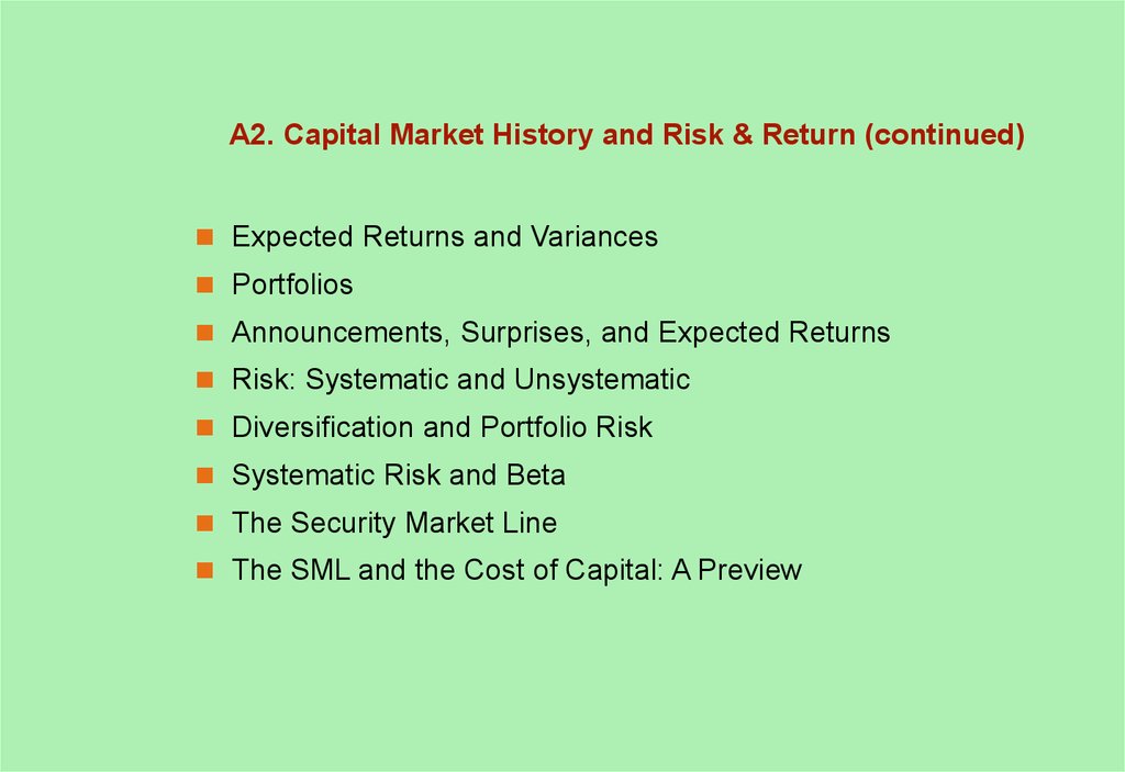
A2. Capital Market History and Risk & Return (continued)
Expected Returns and Variances
Portfolios
Announcements, Surprises, and Expected Returns
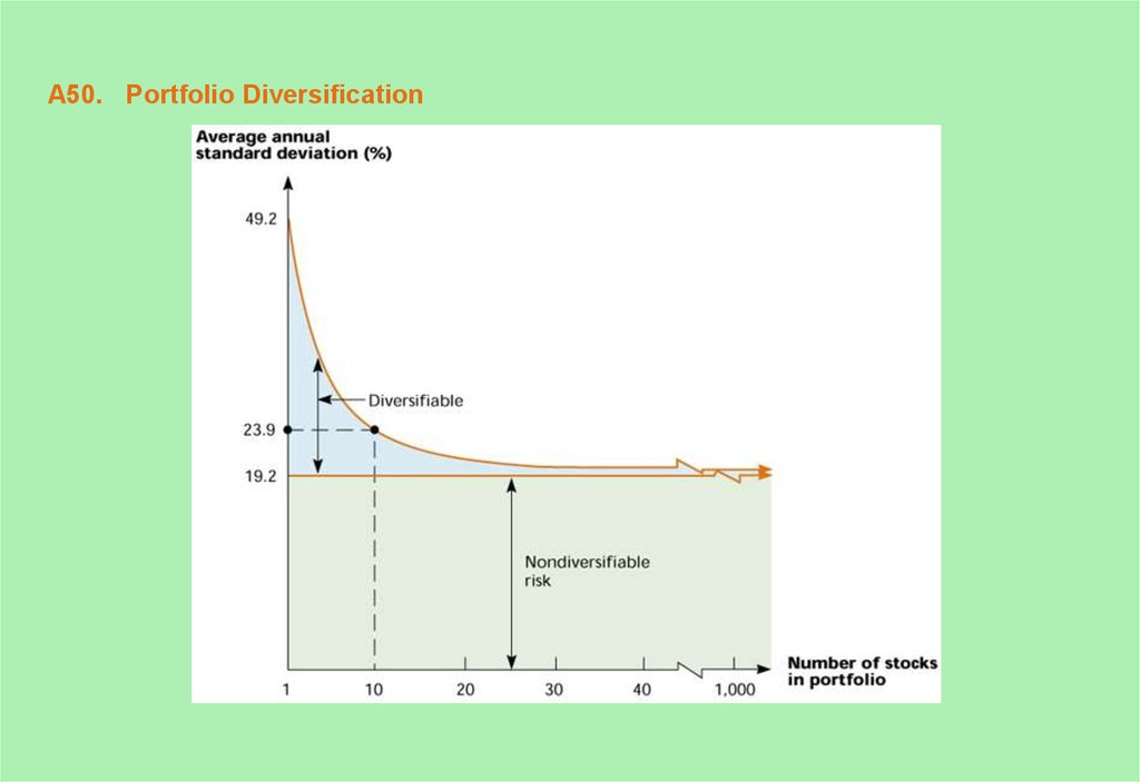
Risk: Systematic and Unsystematic
Diversification and Portfolio Risk
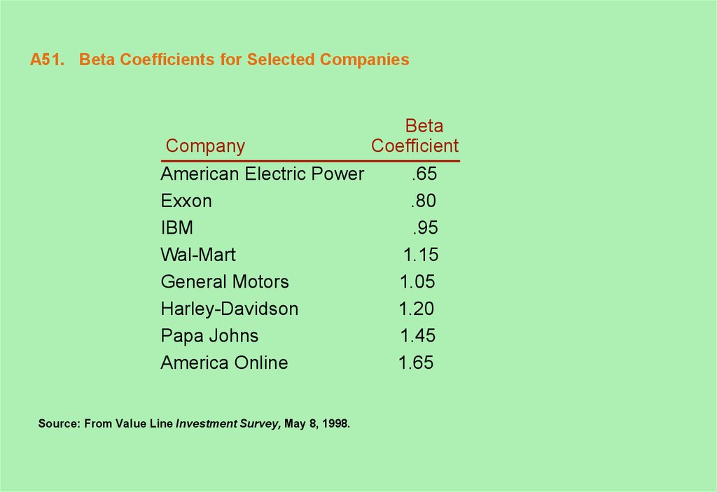
Systematic Risk and Beta
The Security Market Line
The SML and the Cost of Capital: A Preview

3. A3. Risk, Return, and Financial Markets

“. . . Wall Street shapes Main Street. Financial markets
transform factories, department stores, banking assets, film
companies, machinery, soft-drink bottlers, and power lines from
parts of the production process . . . into something easily
convertible into money. Financial markets . . . not only make a
hard asset liquid, they price that asset so as to promote it most
productive use.”
Peter Bernstein, in his book, Capital Ideas

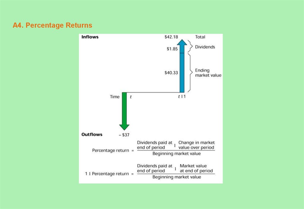
4. A4. Percentage Returns

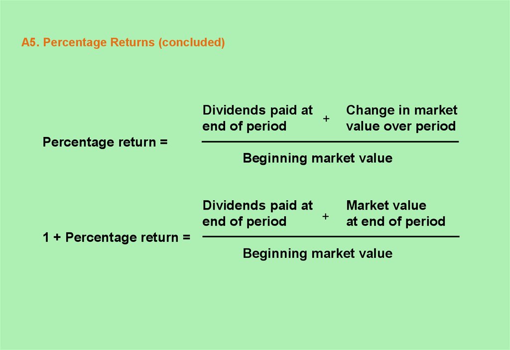
5. A5. Percentage Returns (concluded)

Dividends paid at
+
end of period
Change in market
value over period
Percentage return =
Beginning market value
Dividends paid at
+
end of period
Market value
at end of period
1 + Percentage return =
Beginning market value

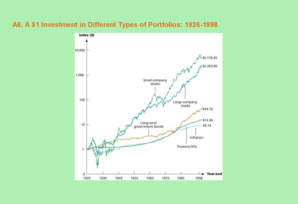
6. A6. A $1 Investment in Different Types of Portfolios: 1926-1998

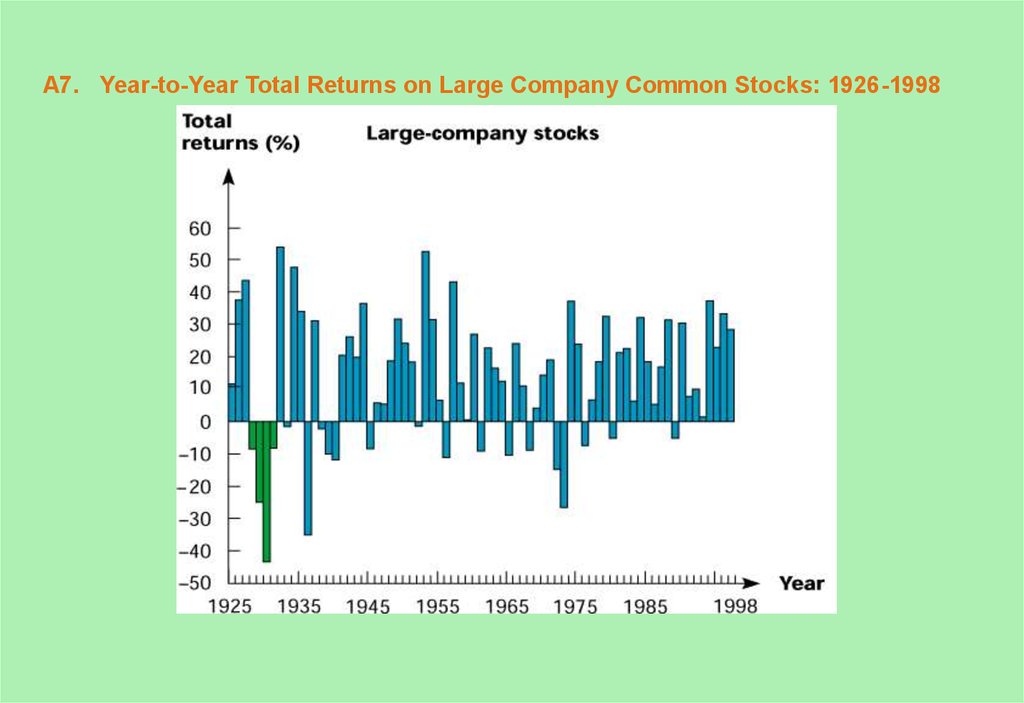
7. A7. Year-to-Year Total Returns on Large Company Common Stocks: 1926-1998

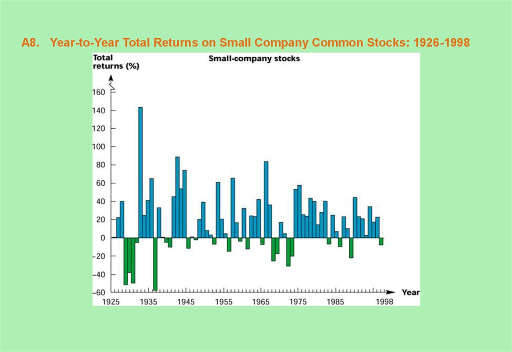
8. A8. Year-to-Year Total Returns on Small Company Common Stocks: 1926-1998

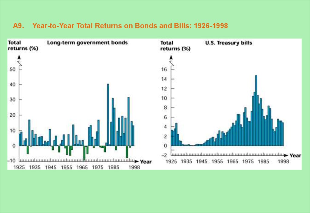
9. A9. Year-to-Year Total Returns on Bonds and Bills: 1926-1998

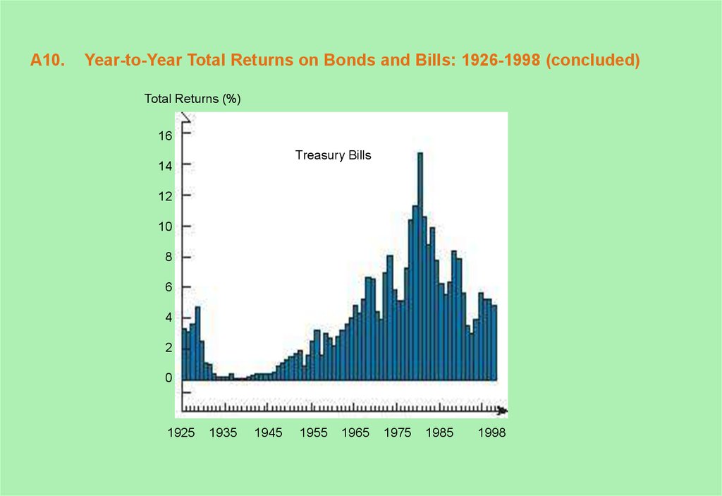
10. A10. Year-to-Year Total Returns on Bonds and Bills: 1926-1998 (concluded)

Total Returns (%)
16
Treasury Bills
14
12
10
8
6
4
2
0
1925
1935
1945
1955
1965
1975
1985
1998

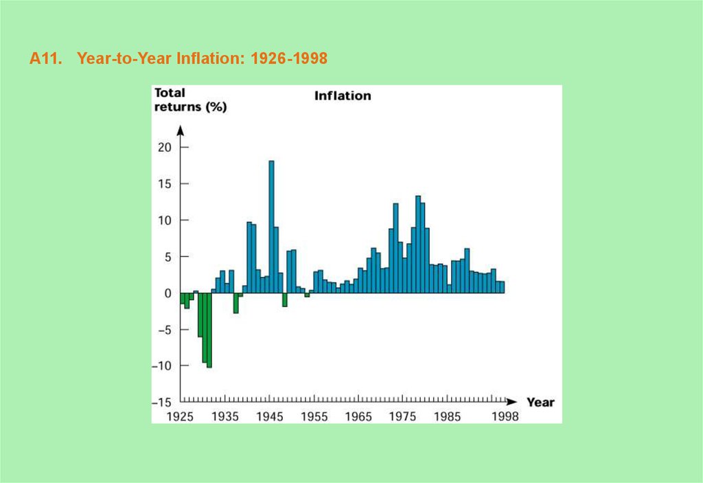
11. A11. Year-to-Year Inflation: 1926-1998

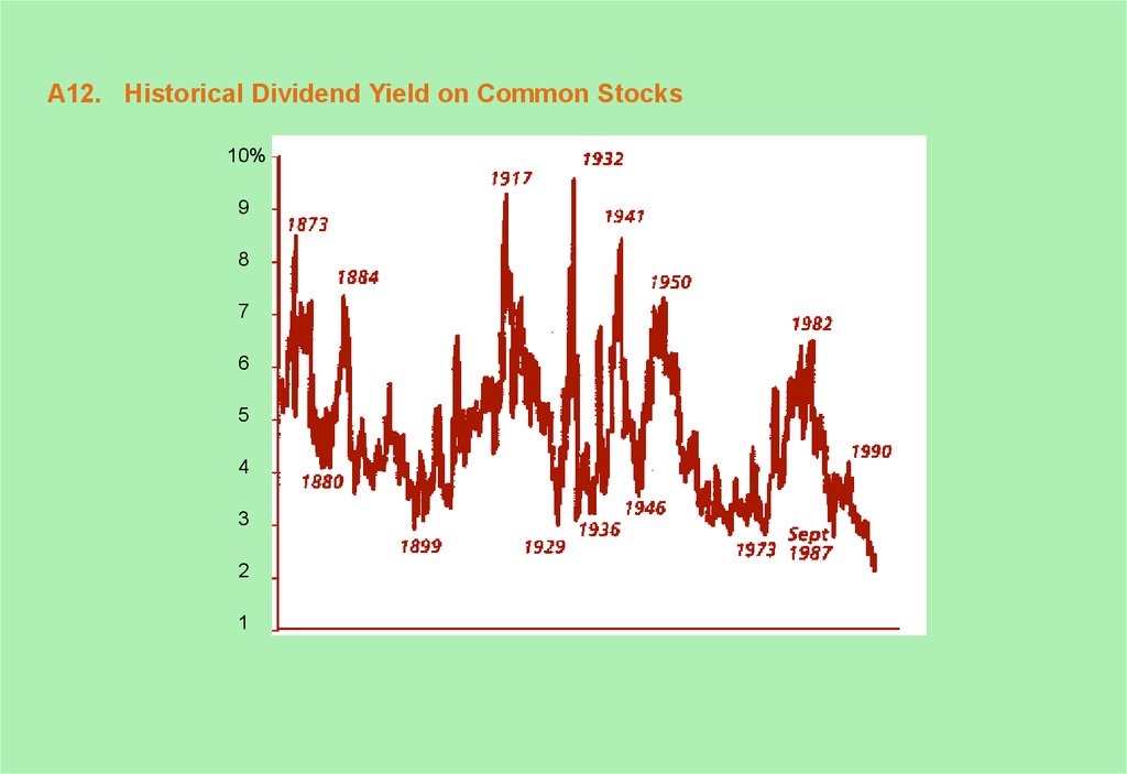
12. A12. Historical Dividend Yield on Common Stocks

10%
9
8
7
6
5
4
3
2
1

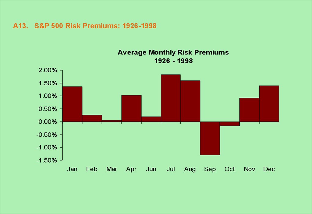
13. A13. S&P 500 Risk Premiums: 1926-1998

A13. S&P 500 Risk Premiums: 1926-1998
Average Monthly Risk Premiums
1926 - 1998
2.00%
1.50%
1.00%
0.50%
0.00%
-0.50%
-1.00%
-1.50%
Jan
Feb
Mar
Apr
Jun
Jul
Aug
Sep
Oct
Nov
Dec

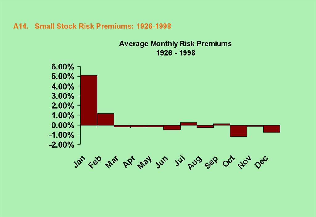
14. A14. Small Stock Risk Premiums: 1926-1998

Average Monthly Risk Premiums
1926 - 1998
D
ec
Ju
l
A
ug
Se
p
O
ct
N
ov
Ju
n
Ja
n
Fe
b
M
ar
A
pr
M
ay
6.00%
5.00%
4.00%
3.00%
2.00%
1.00%
0.00%
-1.00%
-2.00%

15. A15. Using Capital Market History

Now let’s use our knowledge of capital market history to make
some financial decisions. Consider these questions:
Suppose the current T-bill rate is 5%. An investment has
“average” risk relative to a typical share of stock. It offers a
10% return. Is this a good investment?
Suppose an investment is similar in risk to buying small
company equities. If the T-bill rate is 5%, what return would
you demand?

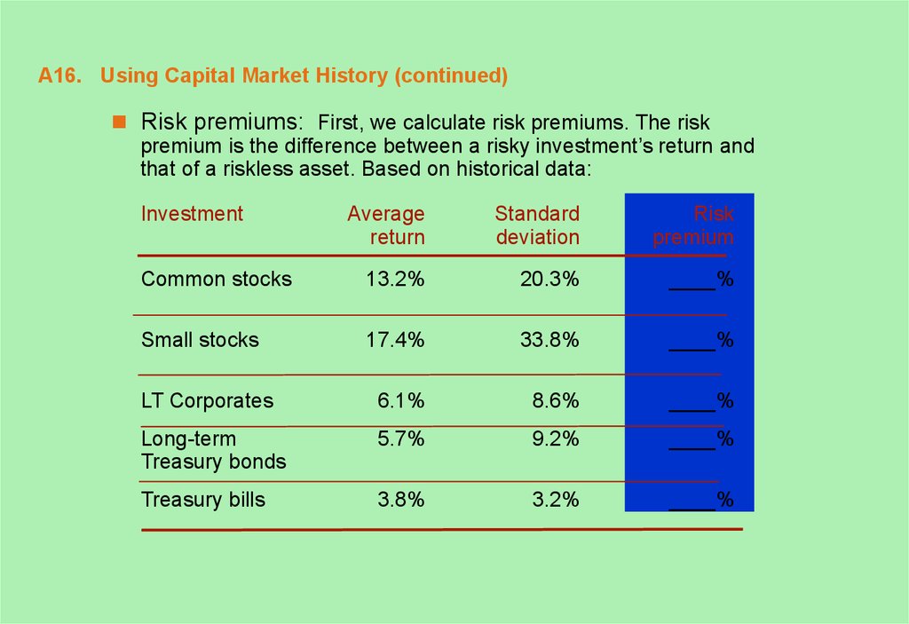
16. A16. Using Capital Market History (continued)

Risk premiums: First, we calculate risk premiums. The risk
premium is the difference between a risky investment’s return and
that of a riskless asset. Based on historical data:
Investment
Average
return
Standard
deviation
Risk
premium
Common stocks
13.2%
20.3%
____%
Small stocks
17.4%
33.8%
____%
LT Corporates
6.1%
8.6%
____%
Long-term
Treasury bonds
5.7%
9.2%
____%
Treasury bills
3.8%
3.2%
____%

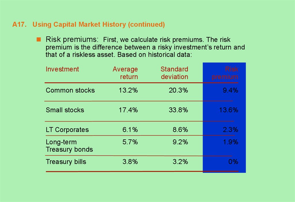
17. A17. Using Capital Market History (continued)

Risk premiums: First, we calculate risk premiums. The risk
premium is the difference between a risky investment’s return and
that of a riskless asset. Based on historical data:
Investment
Average
return
Standard
deviation
Risk
premium
Common stocks
13.2%
20.3%
9.4%
Small stocks
17.4%
33.8%
13.6%
LT Corporates
6.1%
8.6%
2.3%
Long-term
Treasury bonds
5.7%
9.2%
1.9%
Treasury bills
3.8%
3.2%
0%

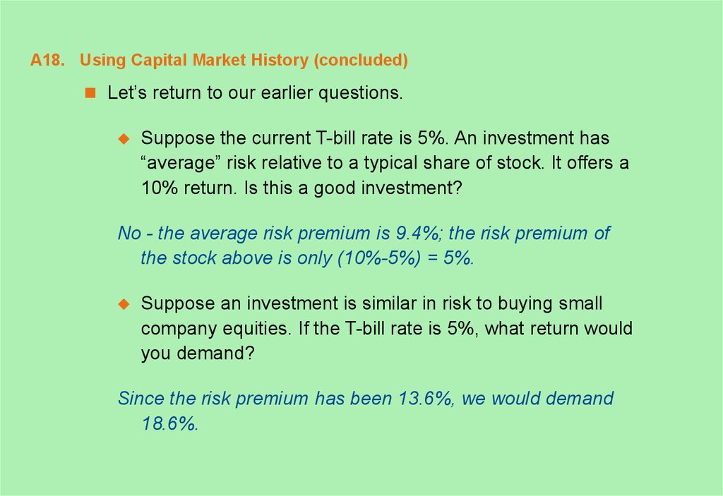
18. A18. Using Capital Market History (concluded)

Let’s return to our earlier questions.
Suppose the current T-bill rate is 5%. An investment has
“average” risk relative to a typical share of stock. It offers a
10% return. Is this a good investment?
No - the average risk premium is 9.4%; the risk premium of
the stock above is only (10%-5%) = 5%.
Suppose an investment is similar in risk to buying small
company equities. If the T-bill rate is 5%, what return would
you demand?
Since the risk premium has been 13.6%, we would demand
18.6%.

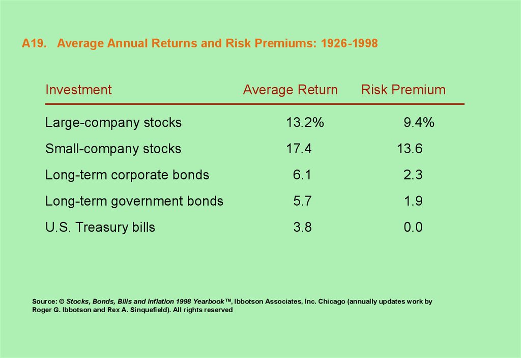
19. A19. Average Annual Returns and Risk Premiums: 1926-1998

Investment
Average Return
Risk Premium
Large-company stocks
13.2%
9.4%
Small-company stocks
17.4
13.6
Long-term corporate bonds
6.1
2.3
Long-term government bonds
5.7
1.9
U.S. Treasury bills
3.8
0.0
Source: © Stocks, Bonds, Bills and Inflation 1998 Yearbook™, Ibbotson Associates, Inc. Chicago (annually updates work by
Roger G. Ibbotson and Rex A. Sinquefield). All rights reserved

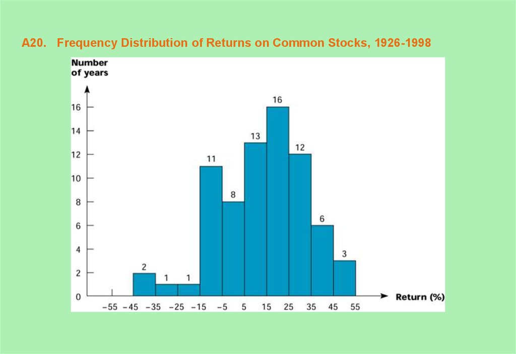
20. A20. Frequency Distribution of Returns on Common Stocks, 1926-1998

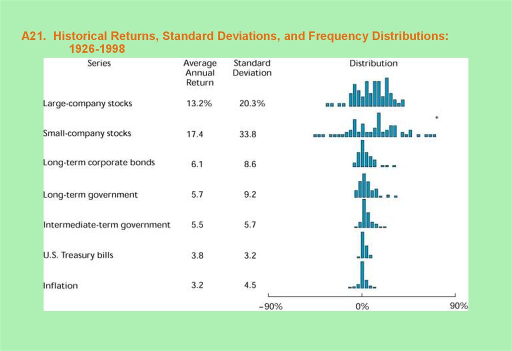
21. A21. Historical Returns, Standard Deviations, and Frequency Distributions: 1926-1998

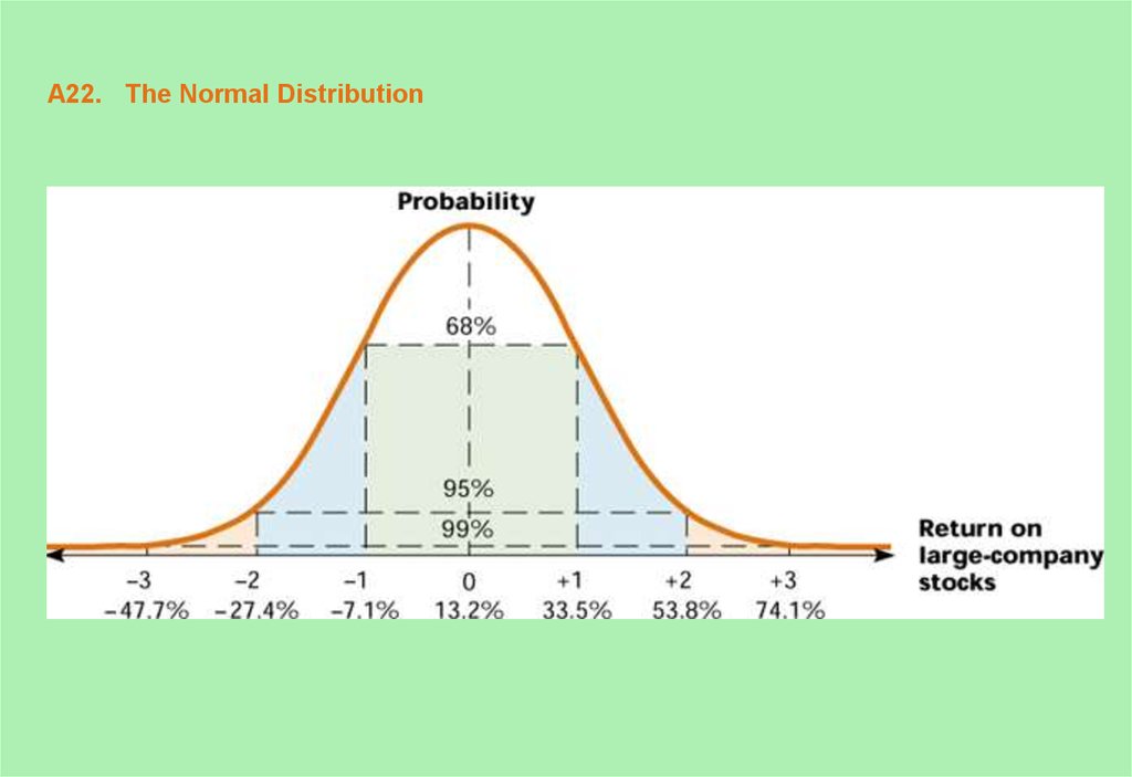
22. A22. The Normal Distribution

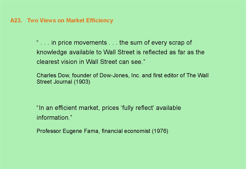
23. A23. Two Views on Market Efficiency

“ . . . in price movements . . . the sum of every scrap of
knowledge available to Wall Street is reflected as far as the
clearest vision in Wall Street can see.”
Charles Dow, founder of Dow-Jones, Inc. and first editor of The Wall
Street Journal (1903)
“In an efficient market, prices ‘fully reflect’ available
information.”
Professor Eugene Fama, financial economist (1976)

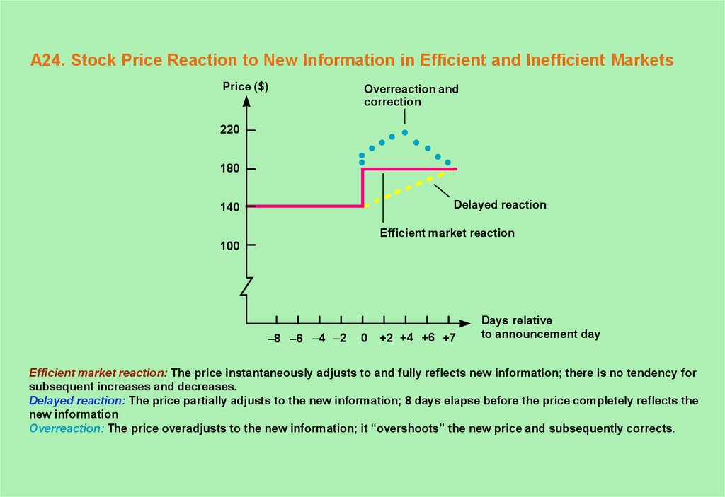
24. A24. Stock Price Reaction to New Information in Efficient and Inefficient Markets

Price ($)
Overreaction and
correction
220
180
Delayed reaction
140
Efficient market reaction
100
–8 –6 –4 –2
0
+2 +4 +6 +7
Days relative
to announcement day
Efficient market reaction: The price instantaneously adjusts to and fully reflects new information; there is no tendency for
subsequent increases and decreases.
Delayed reaction: The price partially adjusts to the new information; 8 days elapse before the price completely reflects the
new information
Overreaction: The price overadjusts to the new information; it “overshoots” the new price and subsequently corrects.

25. A25. A Quick Quiz

Here are three questions that should be easy to answer (if you’ve
been paying attention, that is).
1. How are average annual returns measured?
2. How is volatility measured?
3. Assume your portfolio has had returns of 11%, -8%, 20%, and 10% over the last four years. What is the average annual return?

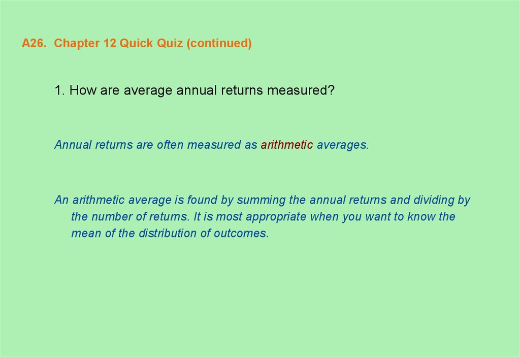
26. A26. Chapter 12 Quick Quiz (continued)

1. How are average annual returns measured?
Annual returns are often measured as arithmetic averages.
An arithmetic average is found by summing the annual returns and dividing by
the number of returns. It is most appropriate when you want to know the
mean of the distribution of outcomes.

27. A27. Chapter 12 Quick Quiz (continued)

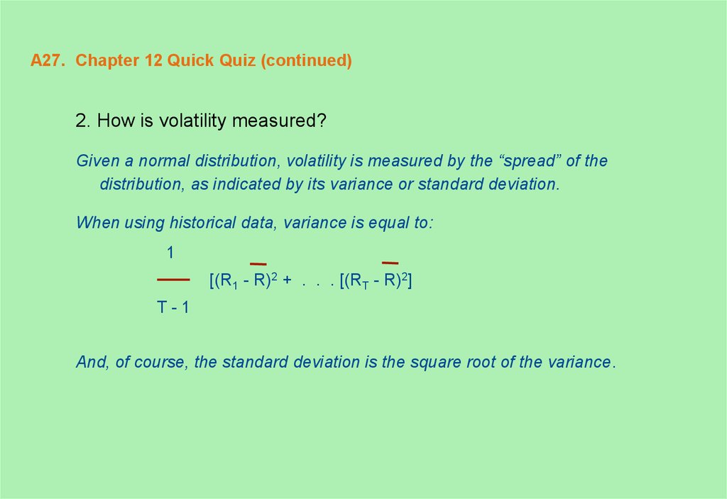
2. How is volatility measured?
Given a normal distribution, volatility is measured by the “spread” of the
distribution, as indicated by its variance or standard deviation.
When using historical data, variance is equal to:
1
[(R1 - R)2 + . . . [(RT - R)2]
T-1
And, of course, the standard deviation is the square root of the variance.

28. A28. Chapter 12 Quick Quiz (concluded)

3. Assume your portfolio has had returns of 11%, -8%, 20%, and
-10% over the last four years. What is the average annual return?
Your average annual return is simply:
[.11 + (-.08) + .20 + (-.10)]/4 = .0325 = 3.25% per year.

29. A29. A Few Examples

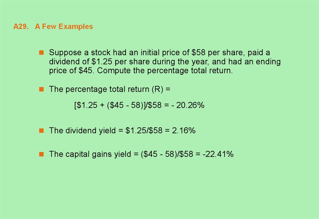
Suppose a stock had an initial price of $58 per share, paid a
dividend of $1.25 per share during the year, and had an ending
price of $45. Compute the percentage total return.
The percentage total return (R) =
[$1.25 + ($45 - 58)]/$58 = - 20.26%
The dividend yield = $1.25/$58 = 2.16%
The capital gains yield = ($45 - 58)/$58 = -22.41%

30. A30. A Few Examples (continued)

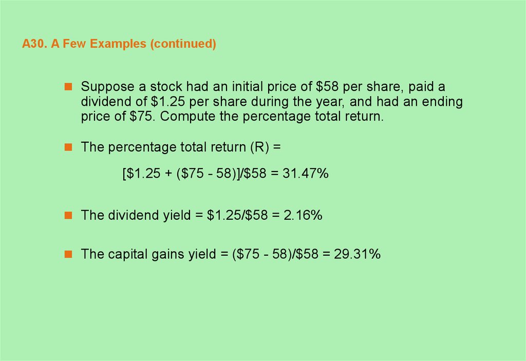
Suppose a stock had an initial price of $58 per share, paid a
dividend of $1.25 per share during the year, and had an ending
price of $75. Compute the percentage total return.
The percentage total return (R) =
[$1.25 + ($75 - 58)]/$58 = 31.47%
The dividend yield = $1.25/$58 = 2.16%
The capital gains yield = ($75 - 58)/$58 = 29.31%

31. A31. A Few Examples (continued)

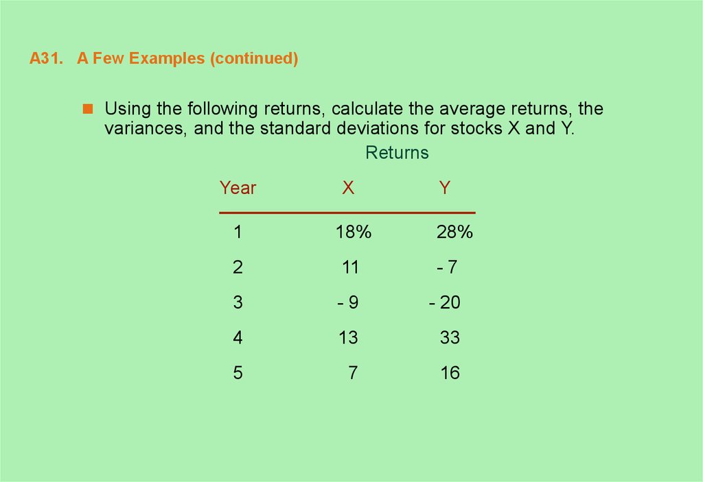
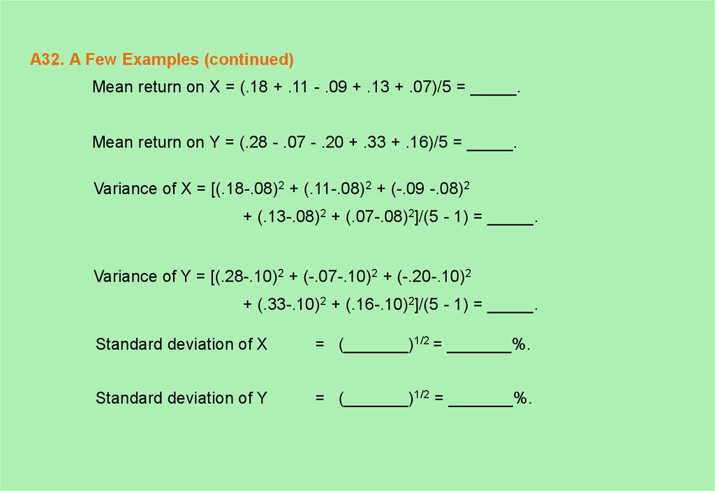
Using the following returns, calculate the average returns, the
variances, and the standard deviations for stocks X and Y.
Returns
Year
X
Y
1
18%
2
11
-7
3
-9
- 20
4
13
33
5
7
16
28%

32. A32. A Few Examples (continued)

Mean return on X = (.18 + .11 - .09 + .13 + .07)/5 = _____.
Mean return on Y = (.28 - .07 - .20 + .33 + .16)/5 = _____.
Variance of X = [(.18-.08)2 + (.11-.08)2 + (-.09 -.08)2
+ (.13-.08)2 + (.07-.08)2]/(5 - 1) = _____.
Variance of Y = [(.28-.10)2 + (-.07-.10)2 + (-.20-.10)2
+ (.33-.10)2 + (.16-.10)2]/(5 - 1) = _____.
Standard deviation of X
= (_______)1/2 = _______%.
Standard deviation of Y
= (_______)1/2 = _______%.

33. A33. A Few Examples (concluded)

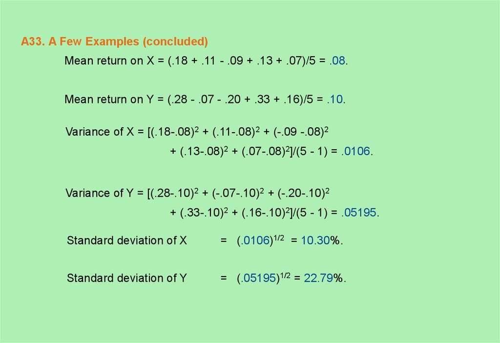
Mean return on X = (.18 + .11 - .09 + .13 + .07)/5 = .08.
Mean return on Y = (.28 - .07 - .20 + .33 + .16)/5 = .10.
Variance of X = [(.18-.08)2 + (.11-.08)2 + (-.09 -.08)2
+ (.13-.08)2 + (.07-.08)2]/(5 - 1) = .0106.
Variance of Y = [(.28-.10)2 + (-.07-.10)2 + (-.20-.10)2
+ (.33-.10)2 + (.16-.10)2]/(5 - 1) = .05195.
Standard deviation of X
= (.0106)1/2 = 10.30%.
Standard deviation of Y
= (.05195)1/2 = 22.79%.

34. A34. Expected Return and Variance: Basic Ideas

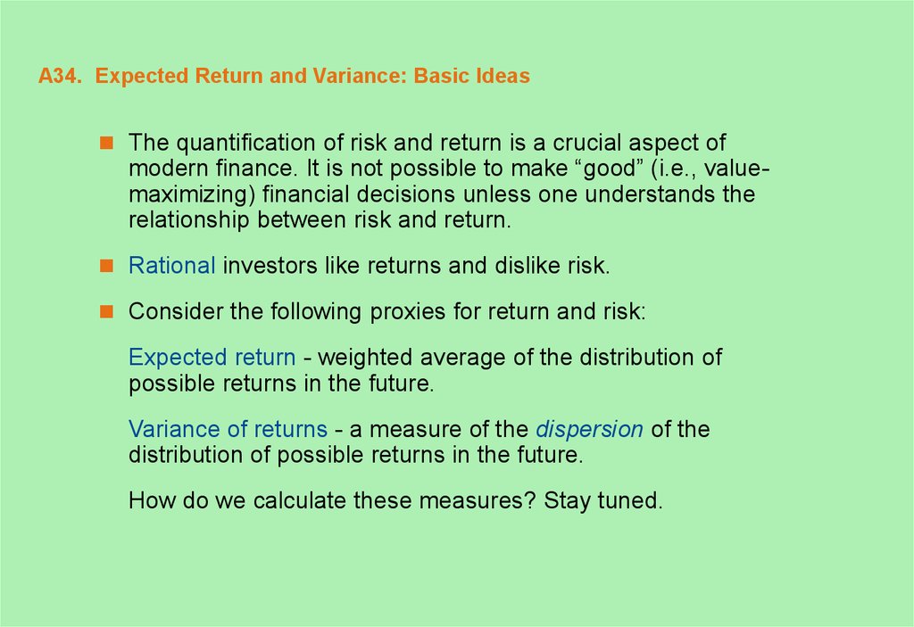
The quantification of risk and return is a crucial aspect of
modern finance. It is not possible to make “good” (i.e., valuemaximizing) financial decisions unless one understands the
relationship between risk and return.
Rational investors like returns and dislike risk.
Consider the following proxies for return and risk:
Expected return - weighted average of the distribution of
possible returns in the future.
Variance of returns - a measure of the dispersion of the
distribution of possible returns in the future.
How do we calculate these measures? Stay tuned.

35. A35. Example: Calculating the Expected Return

pi
Probability
of state i
Ri
Return in
state i
+1% change in GNP
.25
-5%
+2% change in GNP
.50
15%
+3% change in GNP
.25
35%
State of Economy

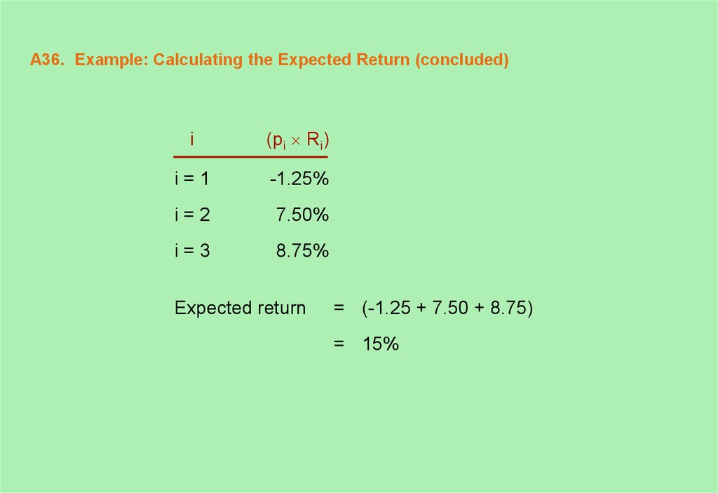
36. A36. Example: Calculating the Expected Return (concluded)

i
(pi Ri)
i=1
-1.25%
i=2
7.50%
i=3
8.75%
Expected return
= (-1.25 + 7.50 + 8.75)
= 15%

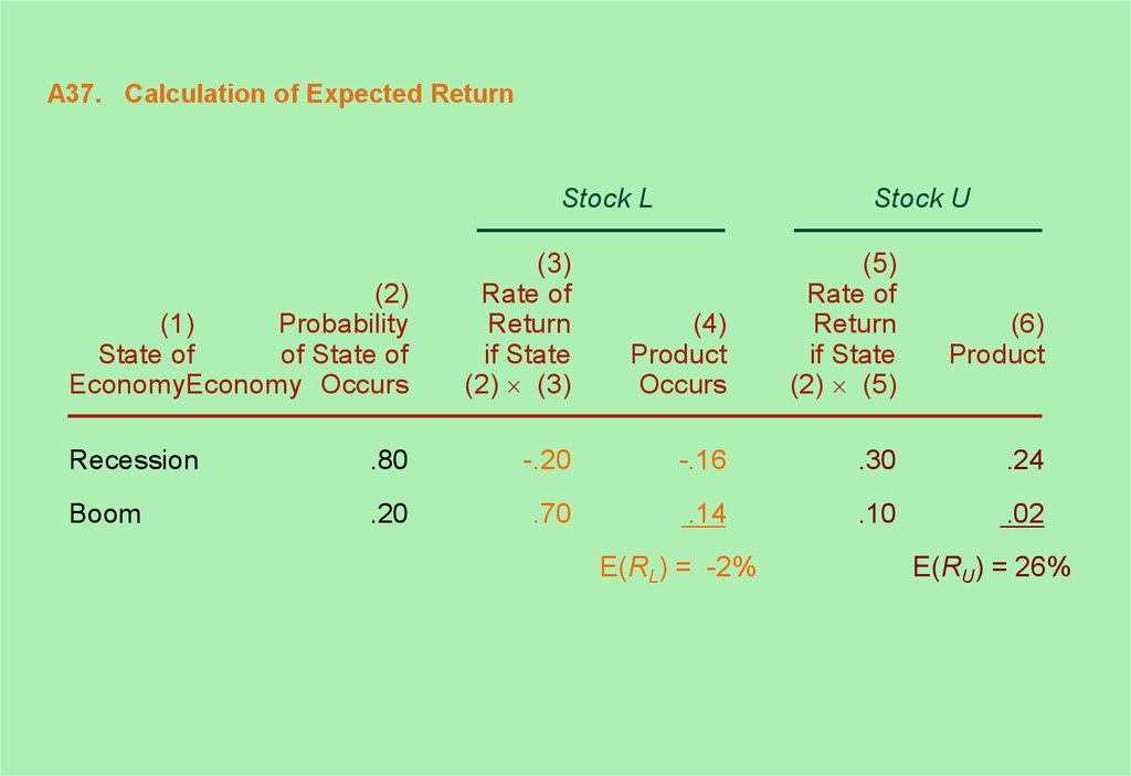
37. A37. Calculation of Expected Return

Stock L
(2)
(1)
Probability
State of
of State of
EconomyEconomy Occurs
Stock U
(3)
Rate of
Return
if State
(2) (3)
(4)
Product
Occurs
(5)
Rate of
Return
if State
(2) (5)
(6)
Product
Recession
.80
-.20
-.16
.30
.24
Boom
.20
.70
.14
.10
.02
E(RL) = -2%
E(RU) = 26%

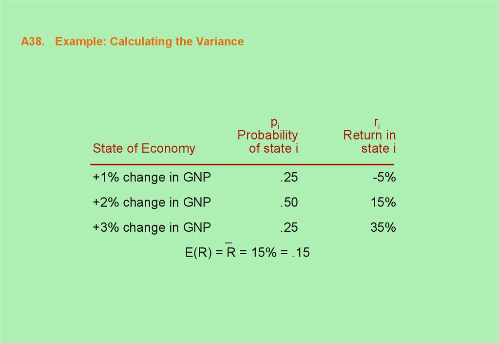
38. A38. Example: Calculating the Variance

pi
Probability
of state i
ri
Return in
state i
+1% change in GNP
.25
-5%
+2% change in GNP
.50
15%
+3% change in GNP
.25
35%
State of Economy
E(R) = R = 15% = .15

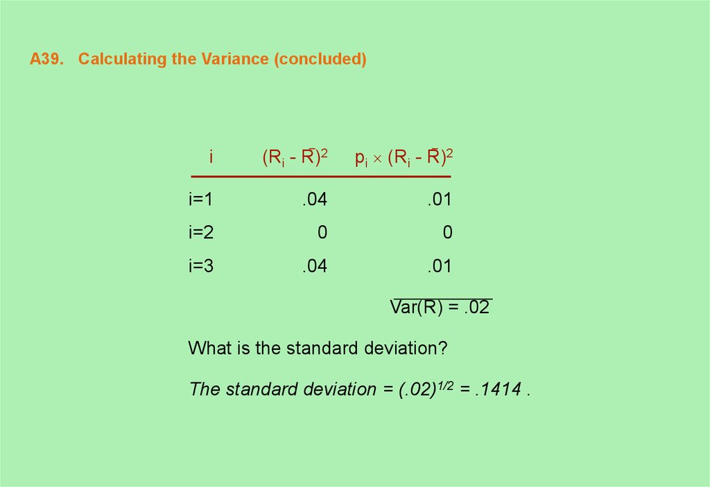
39. A39. Calculating the Variance (concluded)

i
(Ri - R)2
pi (Ri - R)2
i=1
.04
.01
i=2
0
0
i=3
.04
.01
Var(R) = .02
What is the standard deviation?
The standard deviation = (.02)1/2 = .1414 .

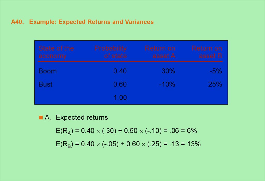
40. A40. Example: Expected Returns and Variances

State of the
economy
Probability
of state
Return on
asset A
Return on
asset B
Boom
0.40
30%
-5%
Bust
0.60
-10%
25%
1.00
A. Expected returns
E(RA) = 0.40 (.30) + 0.60 (-.10) = .06 = 6%
E(RB) = 0.40 (-.05) + 0.60 (.25) = .13 = 13%

41. A41. Example: Expected Returns and Variances (concluded)

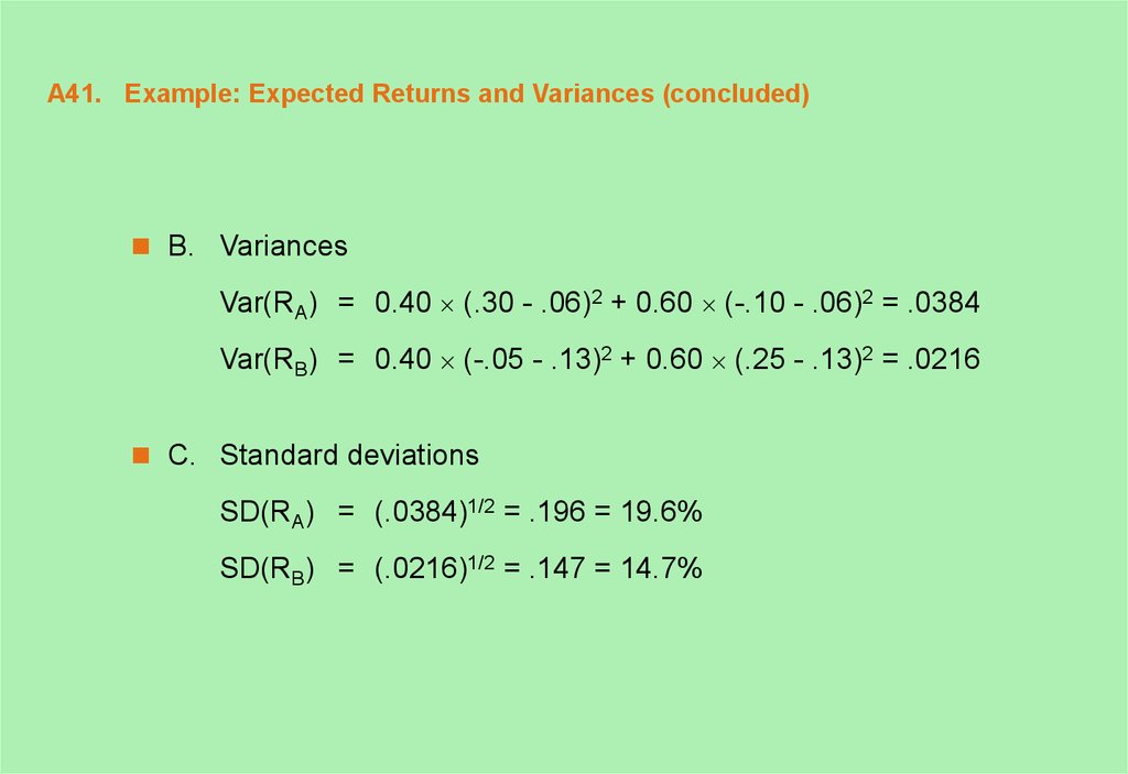
B. Variances
Var(RA) = 0.40 (.30 - .06)2 + 0.60 (-.10 - .06)2 = .0384
Var(RB) = 0.40 (-.05 - .13)2 + 0.60 (.25 - .13)2 = .0216
C. Standard deviations
SD(RA) = (.0384)1/2 = .196 = 19.6%
SD(RB) = (.0216)1/2 = .147 = 14.7%

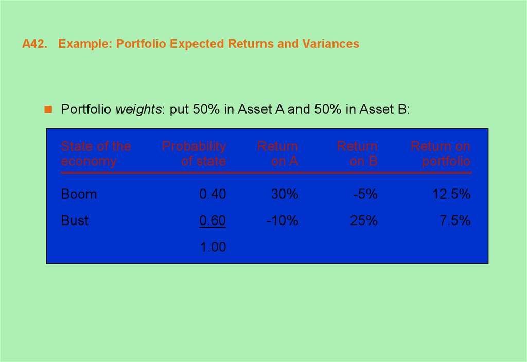
42. A42. Example: Portfolio Expected Returns and Variances

Portfolio weights: put 50% in Asset A and 50% in Asset B:
State of the
economy
Probability
of state
Return
on A
Return
on B
Return on
portfolio
Boom
0.40
30%
-5%
12.5%
Bust
0.60
-10%
25%
7.5%
1.00

43. A43. Example: Portfolio Expected Returns and Variances (continued)

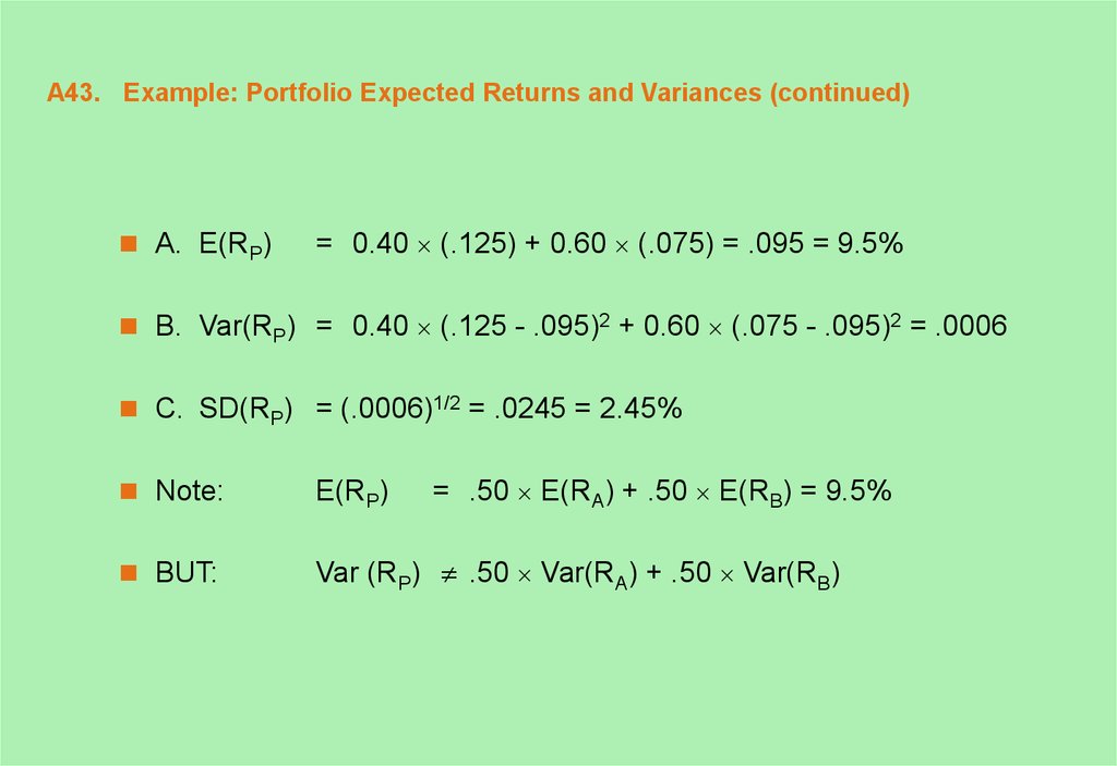
A. E(RP)
= 0.40 (.125) + 0.60 (.075) = .095 = 9.5%
B. Var(RP) = 0.40 (.125 - .095)2 + 0.60 (.075 - .095)2 = .0006
C. SD(RP) = (.0006)1/2 = .0245 = 2.45%
= .50 E(RA) + .50 E(RB) = 9.5%
Note:
E(RP)
BUT:
Var (RP) .50 Var(RA) + .50 Var(RB)

44. A44. Example: Portfolio Expected Returns and Variances (concluded)

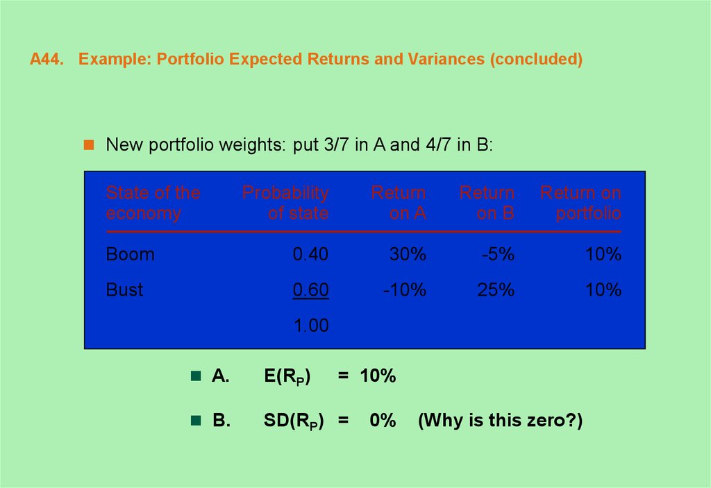
New portfolio weights: put 3/7 in A and 4/7 in B:
State of the
economy
Probability
of state
Return
on A
Return
on B
Return on
portfolio
Boom
0.40
30%
-5%
10%
Bust
0.60
-10%
25%
10%
1.00
A.
E(RP)
B.
SD(RP) =
= 10%
0%
(Why is this zero?)

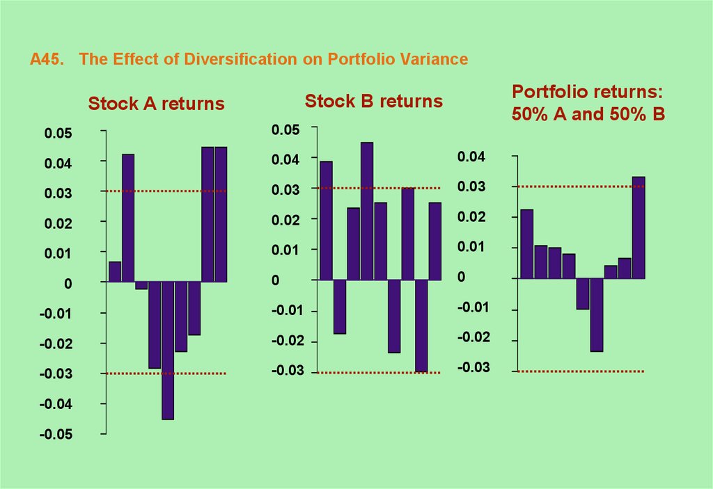
45. A45. The Effect of Diversification on Portfolio Variance

Portfolio returns:
50% A and 50% B
Stock B returns
Stock A returns
0.05
0.05
0.04
0.04
0.04
0.03
0.03
0.03
0.02
0.02
0.02
0.01
0.01
0.01
0
0
-0.01
-0.01
-0.01
-0.02
-0.02
-0.02
-0.03
-0.03
-0.03
0
-0.04
-0.05

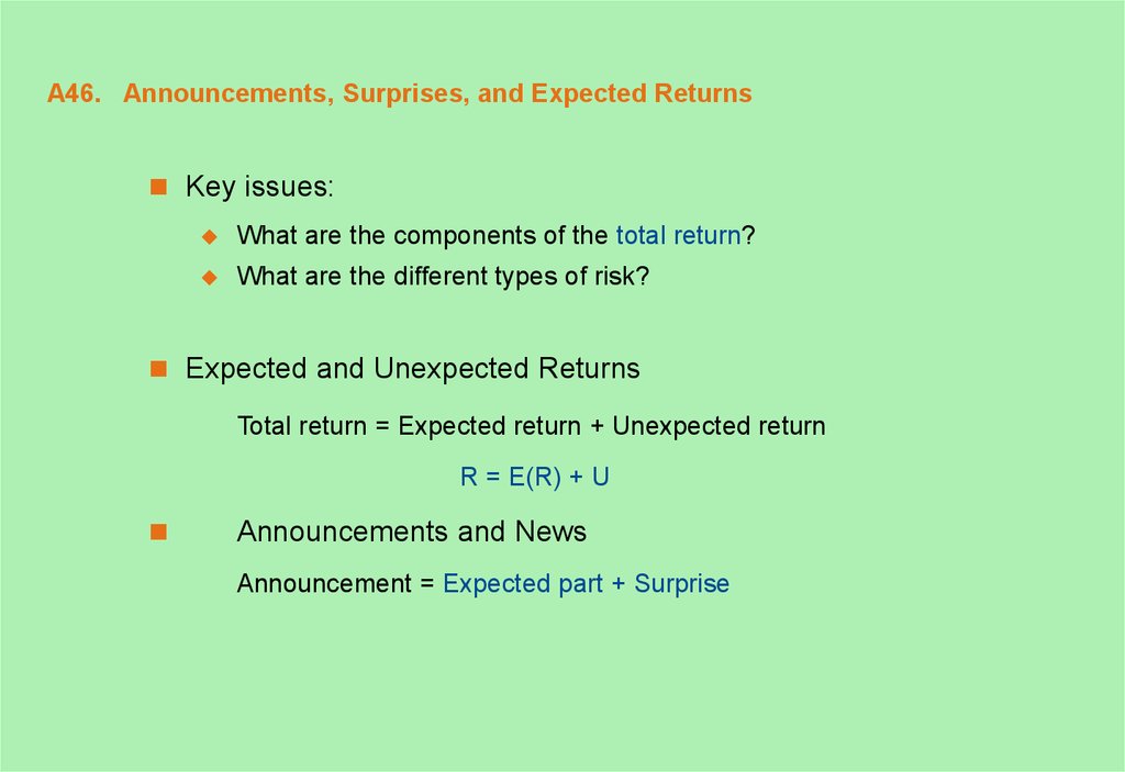
46. A46. Announcements, Surprises, and Expected Returns

Key issues:
What are the components of the total return?
What are the different types of risk?
Expected and Unexpected Returns
Total return = Expected return + Unexpected return
R = E(R) + U
Announcements and News
Announcement = Expected part + Surprise

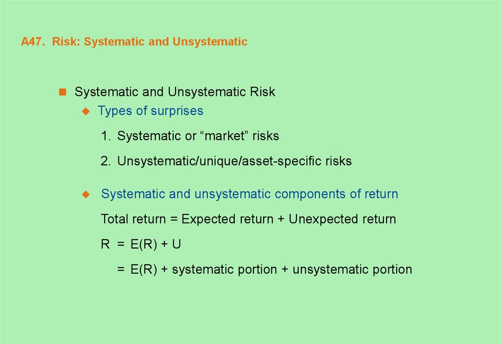
47. A47. Risk: Systematic and Unsystematic

Systematic and Unsystematic Risk
Types of surprises
1. Systematic or “market” risks
2. Unsystematic/unique/asset-specific risks
Systematic and unsystematic components of return
Total return = Expected return + Unexpected return
R = E(R) + U
= E(R) + systematic portion + unsystematic portion

48. A48. Peter Bernstein on Risk and Diversification

“Big risks are scary when you cannot diversify them, especially
when they are expensive to unload; even the wealthiest
families hesitate before deciding which house to buy. Big risks
are not scary to investors who can diversify them; big risks are
interesting. No single loss will make anyone go broke . . . by
making diversification easy and inexpensive, financial markets
enhance the level of risk-taking in society.”
Peter Bernstein, in his book, Capital Ideas

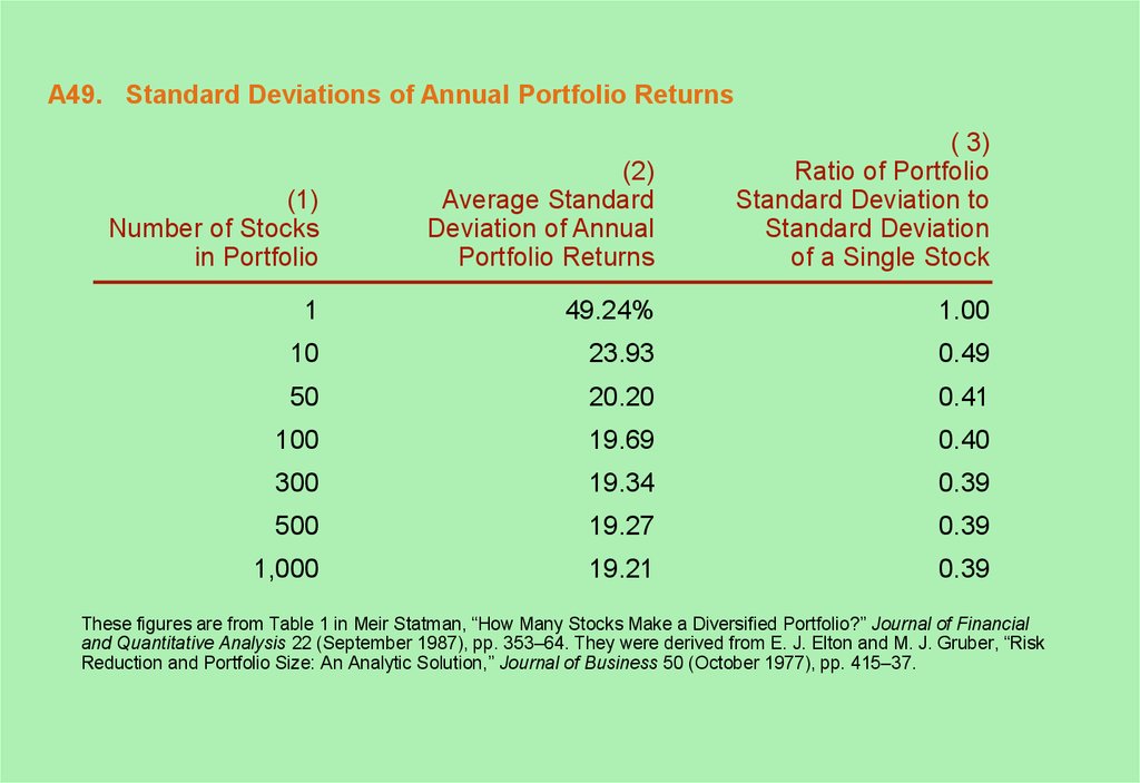
49. A49. Standard Deviations of Annual Portfolio Returns

(1)
Number of Stocks
in Portfolio
(2)
Average Standard
Deviation of Annual
Portfolio Returns
( 3)
Ratio of Portfolio
Standard Deviation to
Standard Deviation
of a Single Stock
1
49.24%
1.00
10
23.93
0.49
50
20.20
0.41
100
19.69
0.40
300
19.34
0.39
500
19.27
0.39
1,000
19.21
0.39
These figures are from Table 1 in Meir Statman, “How Many Stocks Make a Diversified Portfolio?” Journal of Financial
and Quantitative Analysis 22 (September 1987), pp. 353–64. They were derived from E. J. Elton and M. J. Gruber, “Risk
Reduction and Portfolio Size: An Analytic Solution,” Journal of Business 50 (October 1977), pp. 415–37.

50. A50. Portfolio Diversification

51. A51. Beta Coefficients for Selected Companies

Beta
Company
Coefficient
American Electric Power
.65
Exxon
.80
IBM
.95
Wal-Mart
1.15
General Motors
1.05
Harley-Davidson
1.20
Papa Johns
1.45
America Online
1.65
Source: From Value Line Investment Survey, May 8, 1998.

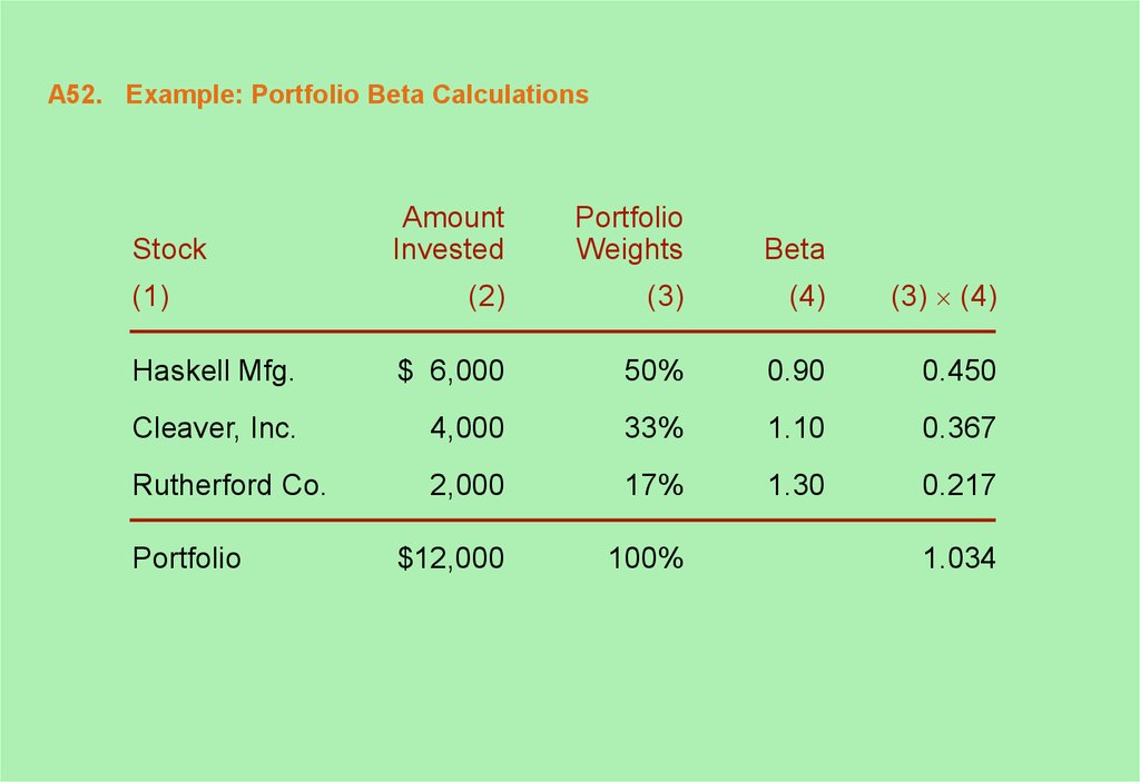
52. A52. Example: Portfolio Beta Calculations

Amount
Invested
Portfolio
Weights
Beta
(2)
(3)
(4)
(3) (4)
Haskell Mfg.
$ 6,000
50%
0.90
0.450
Cleaver, Inc.
4,000
33%
1.10
0.367
Rutherford Co.
2,000
17%
1.30
0.217
$12,000
100%
Stock
(1)
Portfolio
1.034

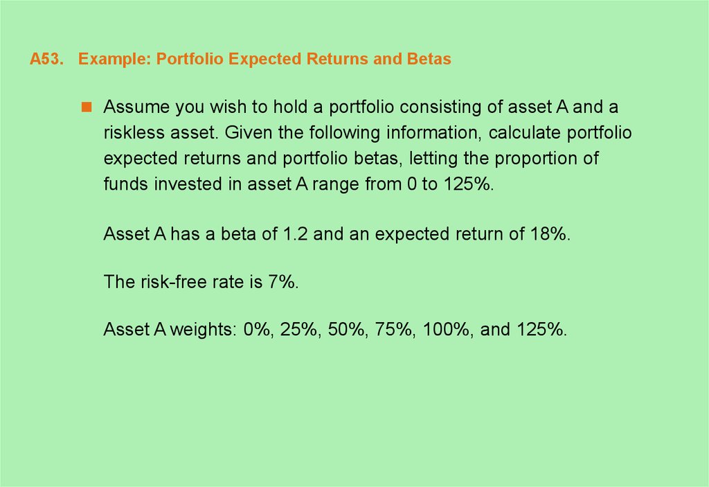
53. A53. Example: Portfolio Expected Returns and Betas

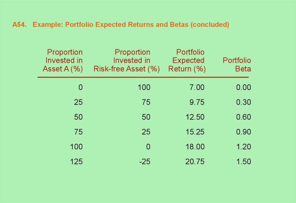
Assume you wish to hold a portfolio consisting of asset A and a
riskless asset. Given the following information, calculate portfolio
expected returns and portfolio betas, letting the proportion of
funds invested in asset A range from 0 to 125%.
Asset A has a beta of 1.2 and an expected return of 18%.
The risk-free rate is 7%.
Asset A weights: 0%, 25%, 50%, 75%, 100%, and 125%.

54. A54. Example: Portfolio Expected Returns and Betas (concluded)

Proportion
Invested in
Asset A (%)
Proportion
Invested in
Risk-free Asset (%)
Portfolio
Expected
Return (%)
Portfolio
Beta
0
100
7.00
0.00
25
75
9.75
0.30
50
50
12.50
0.60
75
25
15.25
0.90
100
0
18.00
1.20
125
-25
20.75
1.50

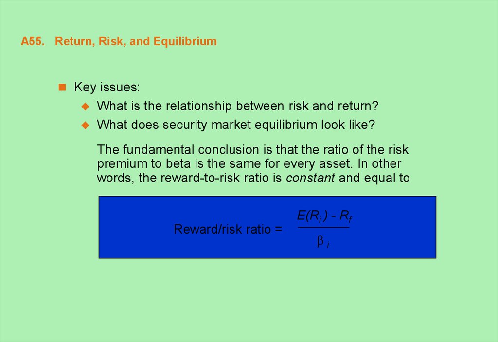
55. A55. Return, Risk, and Equilibrium

Key issues:
What is the relationship between risk and return?
What does security market equilibrium look like?
The fundamental conclusion is that the ratio of the risk
premium to beta is the same for every asset. In other
words, the reward-to-risk ratio is constant and equal to
Reward/risk ratio =
E(Ri ) - Rf
i

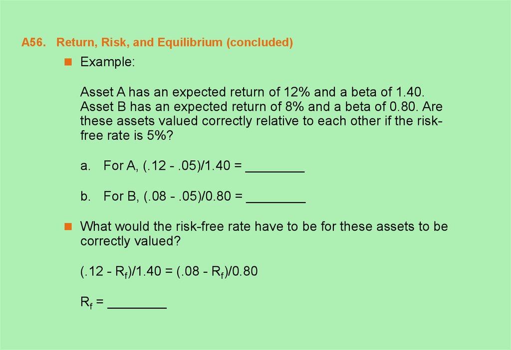
56. A56. Return, Risk, and Equilibrium (concluded)

Example:
Asset A has an expected return of 12% and a beta of 1.40.
Asset B has an expected return of 8% and a beta of 0.80. Are
these assets valued correctly relative to each other if the riskfree rate is 5%?
a. For A, (.12 - .05)/1.40 = ________
b. For B, (.08 - .05)/0.80 = ________
What would the risk-free rate have to be for these assets to be
correctly valued?
(.12 - Rf)/1.40 = (.08 - Rf)/0.80
Rf = ________

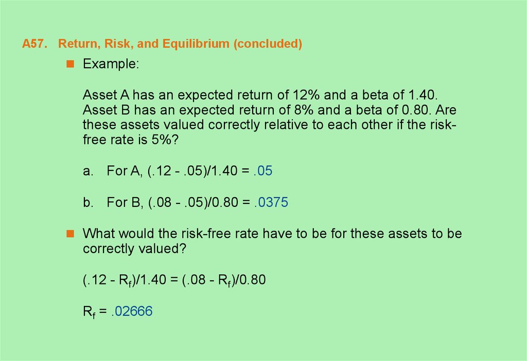
57. A57. Return, Risk, and Equilibrium (concluded)

Example:
Asset A has an expected return of 12% and a beta of 1.40.
Asset B has an expected return of 8% and a beta of 0.80. Are
these assets valued correctly relative to each other if the riskfree rate is 5%?
a. For A, (.12 - .05)/1.40 = .05
b. For B, (.08 - .05)/0.80 = .0375
What would the risk-free rate have to be for these assets to be
correctly valued?
(.12 - Rf)/1.40 = (.08 - Rf)/0.80
Rf = .02666

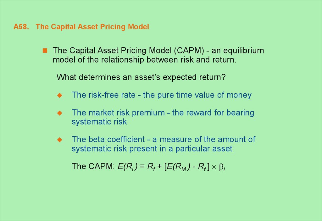
58. A58. The Capital Asset Pricing Model

The Capital Asset Pricing Model (CAPM) - an equilibrium
model of the relationship between risk and return.
What determines an asset’s expected return?
The risk-free rate - the pure time value of money
The market risk premium - the reward for bearing
systematic risk
The beta coefficient - a measure of the amount of
systematic risk present in a particular asset
The CAPM: E(Ri ) = Rf + [E(RM ) - Rf ] i

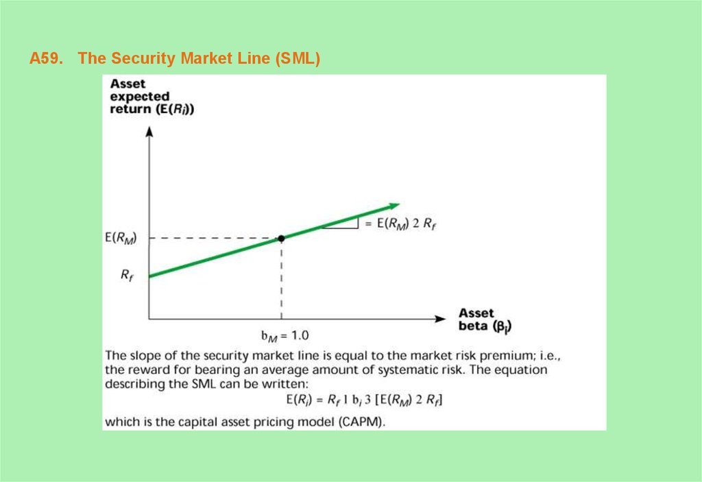
59. A59. The Security Market Line (SML)

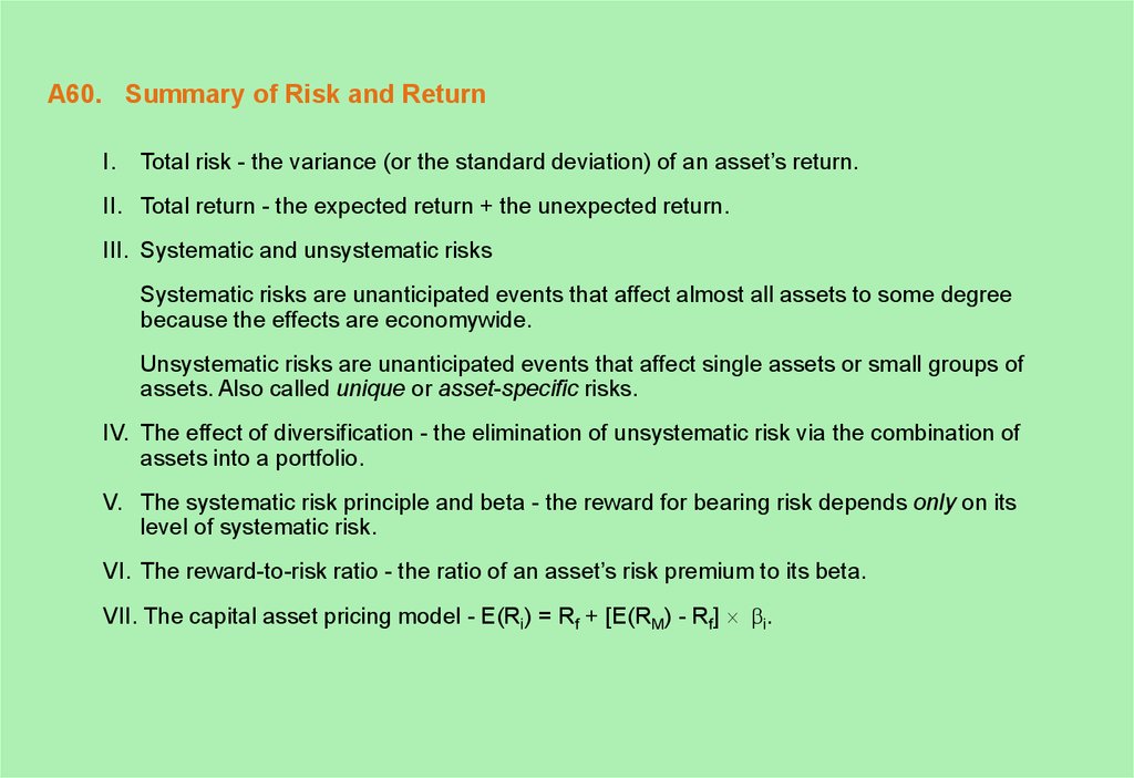
60. A60. Summary of Risk and Return

I.
Total risk - the variance (or the standard deviation) of an asset’s return.
II. Total return - the expected return + the unexpected return.
III. Systematic and unsystematic risks
Systematic risks are unanticipated events that affect almost all assets to some degree
because the effects are economywide.
Unsystematic risks are unanticipated events that affect single assets or small groups of
assets. Also called unique or asset-specific risks.
IV. The effect of diversification - the elimination of unsystematic risk via the combination of
assets into a portfolio.
V. The systematic risk principle and beta - the reward for bearing risk depends only on its
level of systematic risk.
VI. The reward-to-risk ratio - the ratio of an asset’s risk premium to its beta.
VII. The capital asset pricing model - E(Ri) = Rf + [E(RM) - Rf] i.

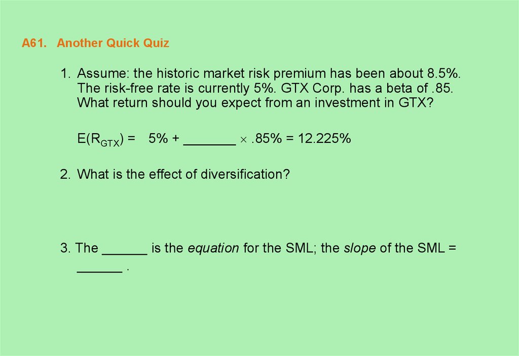
61. A61. Another Quick Quiz

1. Assume: the historic market risk premium has been about 8.5%.
The risk-free rate is currently 5%. GTX Corp. has a beta of .85.
What return should you expect from an investment in GTX?
E(RGTX) = 5% + _______ .85% = 12.225%
2. What is the effect of diversification?
3. The ______ is the equation for the SML; the slope of the SML =
______ .

62. A62. Another Quick Quiz (continued)

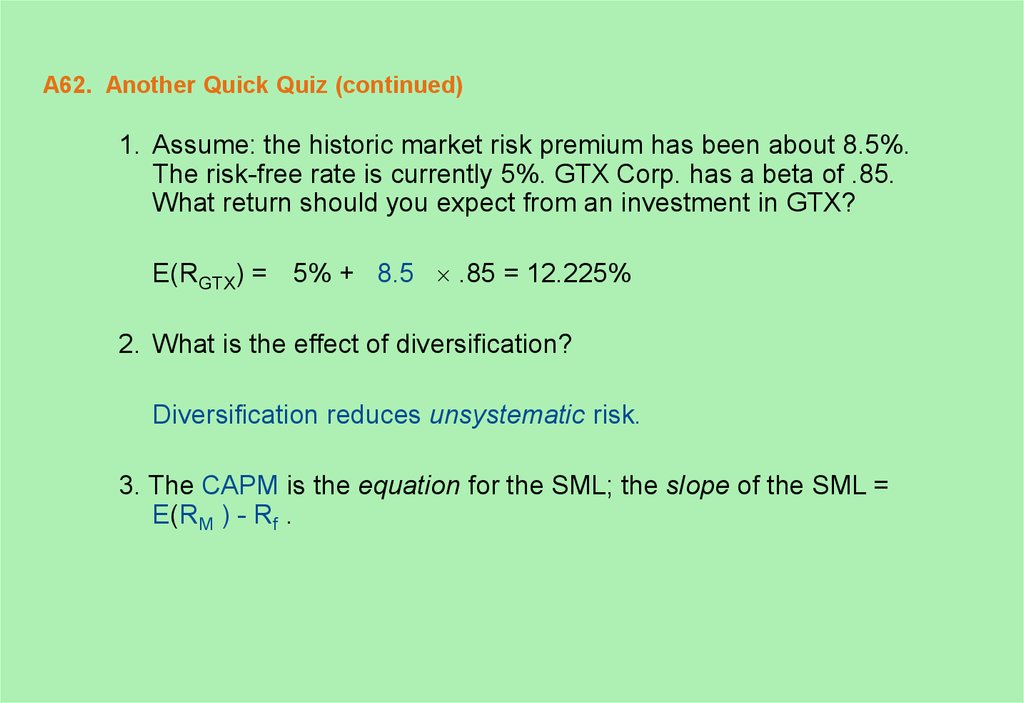
1. Assume: the historic market risk premium has been about 8.5%.
The risk-free rate is currently 5%. GTX Corp. has a beta of .85.
What return should you expect from an investment in GTX?
E(RGTX) = 5% + 8.5 .85 = 12.225%
2. What is the effect of diversification?
Diversification reduces unsystematic risk.
3. The CAPM is the equation for the SML; the slope of the SML =
E(RM ) - Rf .

63. A63. An Example

Consider the following information:
State of
Economy
Prob. of State
of Economy
Stock A
Return
Stock B
Return
Stock C
Return
Boom
0.35
0.14
0.15
0.33
Bust
0.65
0.12
0.03
-0.06
What is the expected return on an equally weighted portfolio of these
three stocks?
What is the variance of a portfolio invested 15 percent each in A and B,
and 70 percent in C?

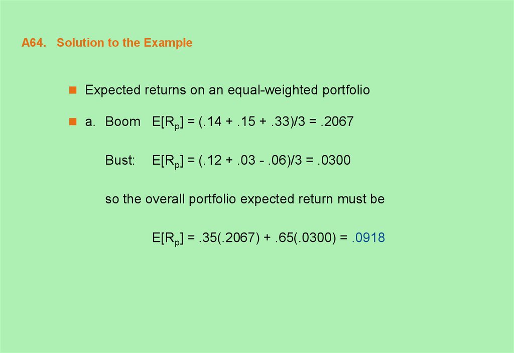
64. A64. Solution to the Example

Expected returns on an equal-weighted portfolio
a. Boom E[Rp] = (.14 + .15 + .33)/3 = .2067
Bust:
E[Rp] = (.12 + .03 - .06)/3 = .0300
so the overall portfolio expected return must be
E[Rp] = .35(.2067) + .65(.0300) = .0918

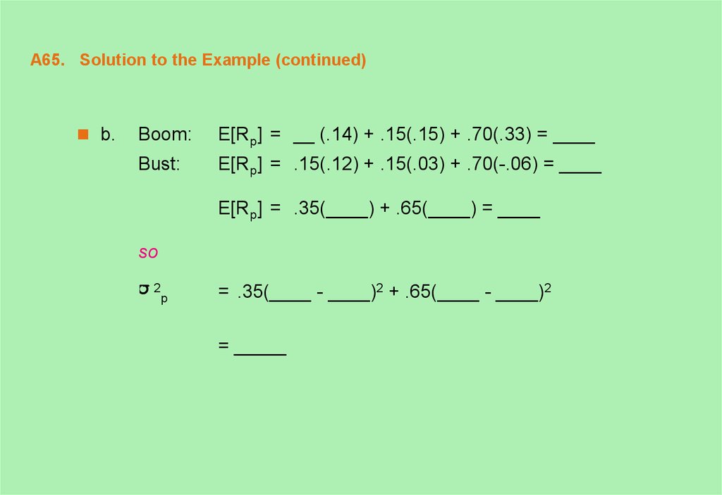
65. A65. Solution to the Example (continued)

b.
Boom:
E[Rp] = __ (.14) + .15(.15) + .70(.33) = ____
Bust:
E[Rp] = .15(.12) + .15(.03) + .70(-.06) = ____
E[Rp] = .35(____) + .65(____) = ____
so
2
p
= .35(____ - ____)2 + .65(____ - ____)2
= _____

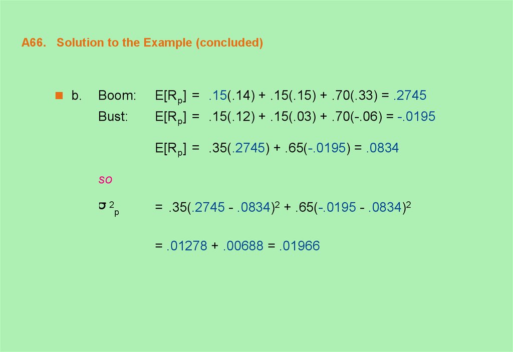
66. A66. Solution to the Example (concluded)

b.
Boom:
E[Rp] = .15(.14) + .15(.15) + .70(.33) = .2745
Bust:
E[Rp] = .15(.12) + .15(.03) + .70(-.06) = -.0195
E[Rp] = .35(.2745) + .65(-.0195) = .0834
so
2
p
= .35(.2745 - .0834)2 + .65(-.0195 - .0834)2
= .01278 + .00688 = .01966

67. A67. Another Example

Using information from capital market history, determine the
return on a portfolio that was equally invested in largecompany stocks and long-term government bonds.
What was the return on a portfolio that was equally invested in
small company stocks and Treasury bills?

68. A68. Solution to the Example

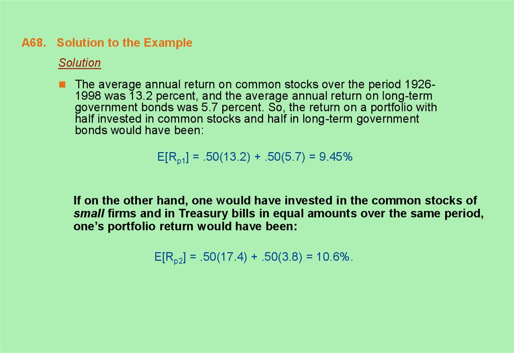
Solution
The average annual return on common stocks over the period 1926-
1998 was 13.2 percent, and the average annual return on long-term
government bonds was 5.7 percent. So, the return on a portfolio with
half invested in common stocks and half in long-term government
bonds would have been:
E[Rp1] = .50(13.2) + .50(5.7) = 9.45%
If on the other hand, one would have invested in the common stocks of
small firms and in Treasury bills in equal amounts over the same period,
one’s portfolio return would have been:
E[Rp2] = .50(17.4) + .50(3.8) = 10.6%.