1.45M

Category: $mathematics$ mathematics

Probability theory. Probability Distributions Statistical Entropy

1.

MEPhI General Physics
Molecular Physics. Statistics
Lecture 08
Probability theory.
Probability Distributions
Statistical Entropy

Thermodynamics and Physical Statistics
Thermodynamic Approach
- defines correlations between the
observed physical quantities
(macroscopic),
- relies mostly on the
experimentally established
dependencies
- allows generally to consider the
physical essence of the problem - does not require precise
information about the microscopic
structure of matter.

3.

Thermodynamics and Physical Statistics
Statistical Approach
Thermodynamic Approach
- defines correlations between the observed physical quantities
(macroscopic),
- relies mostly on the
experimentally established
dependencies
- allows generally to consider the
physical essence of the problem - does not require precise
information about the microscopic
structure of matter.
Based on certain models of the
micro-structure of matter
defines correlations between the
observed physical quantities,
starting from the laws of motion of
molecules using the methods of
probability theory and mathematical
statistics
allows to understand the random
fluctuations of macroscopic
parameters.

4.

5.

Probabilities
Probability = the quantitative measure of possibility for certain event to occur.
EXAMPLE 1. Eagle and Tails Game:
Test = throw of a coin;
Results of a test (events); eagle.
or tail
If the game is honest – possibilities to obtain each result must be equal.
Quantitative measure of possibility = probability: Pe=0,5 – eagle; Pt=0,5 - tail.
P = 1 is the probability of a “valid” event, which will occur for sure.
Pe + Pt=1 – either eagle or tail will fall out for sure (if rib is excluded ).
The rule of adding probabilities P (1 OR 2) = P(1) + P(2)
The normalization rule: the sum of probabilities for all possible results of a test
is evidently valid and thus is equal to 1.

6.

Probabilities
Probability = he quantitative measure of possibility for certain event to occur.
EXAMPLE 2. Dice game. Test = throw of a dice;
Results of a test (events); 1, 2, 3, 4, 5, 6
If the game is “honest”: P(1) = P(2) = P(3) = P(4) = P(5) = P(6) = 1/6.
Example 2.1: Probability to obtain the odd number as the result of a test:
P(1) + P(3) + P(5) = 1/6 + 1/6 + 1/6 = 1/2
Example 2.2: Probability to obtain “double 6”: from the first throw P(6) = 1/6,
and then – out of this probability only 1/6 of chances that 6 will occur again.
Finally P( 6 AND 6) = P(6)P(6) = 1/6*1/6 = 1/36
The rule of multiplying probabilities P (1 AND 2) = P(1)P(2)

7.

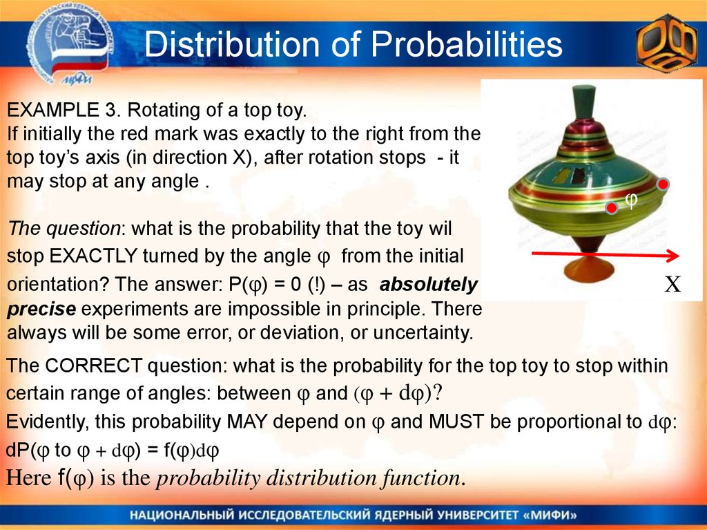
Distribution of Probabilities
EXAMPLE 3. Rotating of a top toy.
If initially the red mark was exactly to the right from the
top toy’s axis (in direction X), after rotation stops - it
may stop at any angle .
The question: what is the probability that the toy wil
stop EXACTLY turned by the angle φ from the initial
orientation? The answer: P(φ) = 0 (!) – as absolutely
precise experiments are impossible in principle. There
always will be some error, or deviation, or uncertainty.
φ
X
The CORRECT question: what is the probability for the top toy to stop within
certain range of angles: between φ and (φ + dφ)?
Evidently, this probability MAY depend on φ and MUST be proportional to dφ:
dP(φ to φ + dφ) = f(φ)dφ
Here f(φ) is the probability distribution function.

8.

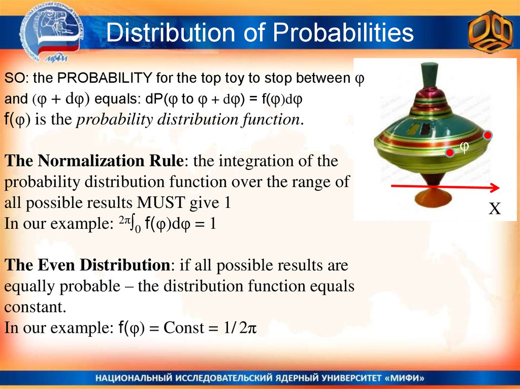
Distribution of Probabilities
SO: the PROBABILITY for the top toy to stop between φ
and (φ + dφ) equals: dP(φ to φ + dφ) = f(φ)dφ
f(φ) is the probability distribution function.
φ
The Normalization Rule: the integration of the
probability distribution function over the range of
all possible results MUST give 1
In our example: 2π∫0 f(φ)dφ = 1
The Even Distribution: if all possible results are
equally probable – the distribution function equals
constant.
In our example: f(φ) = Const = 1/ 2π
X

9.

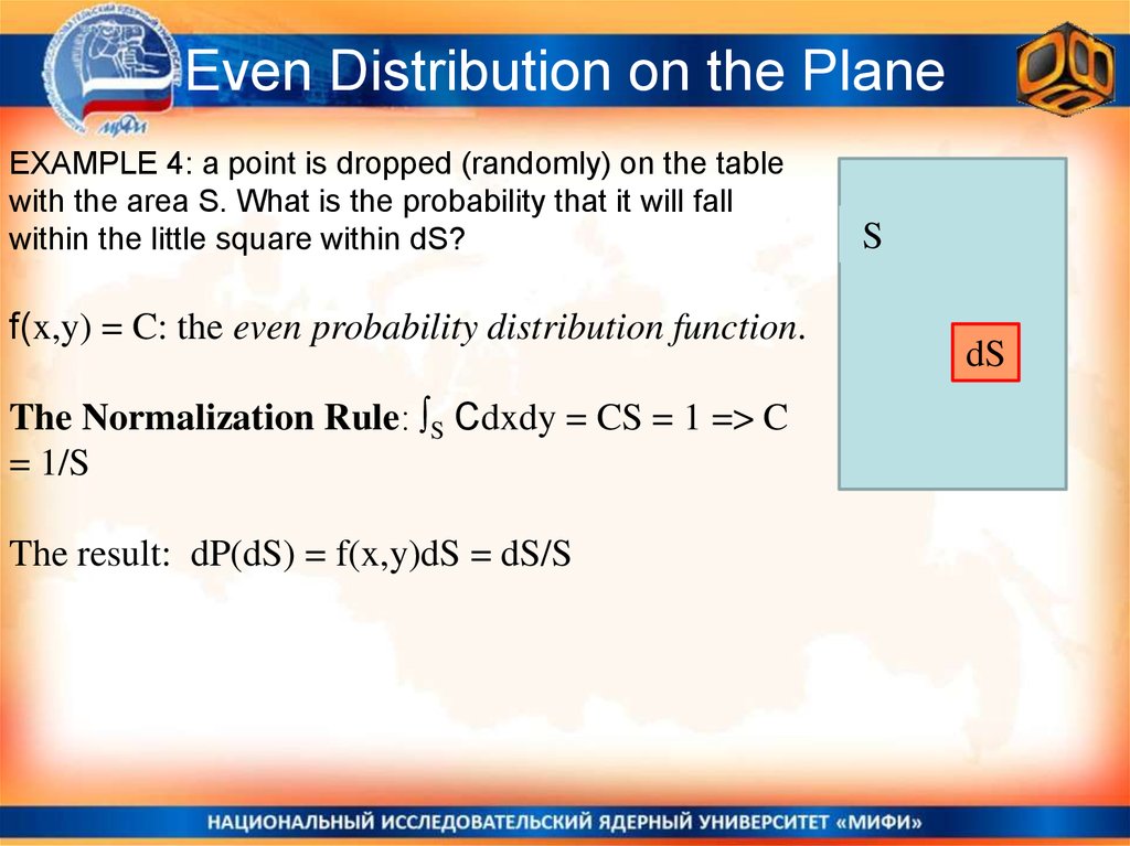
Even Distribution on the Plane
EXAMPLE 4: a point is dropped (randomly) on the table
with the area S. What is the probability that it will fall
within the little square within dS?
f(x,y) = C: the even probability distribution function.
The Normalization Rule: ∫S Cdxdy = CS = 1 => C
= 1/S
The result: dP(dS) = f(x,y)dS = dS/S
S
dS

10.

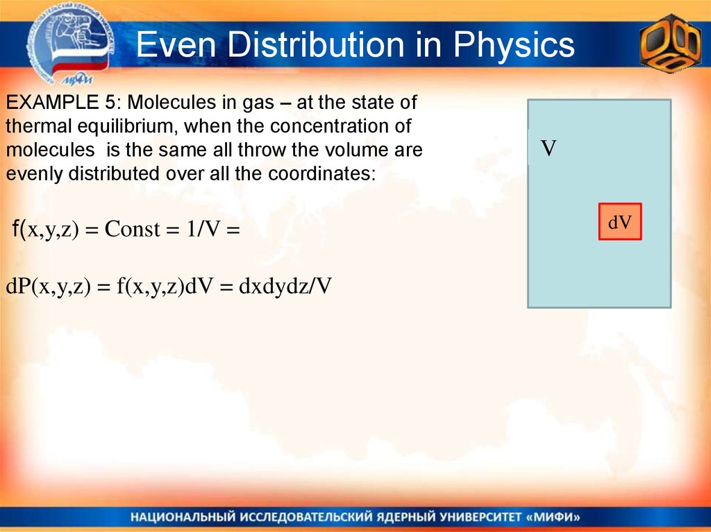
Even Distribution in Physics
EXAMPLE 5: Molecules in gas – at the state of
thermal equilibrium, when the concentration of
molecules is the same all throw the volume are
evenly distributed over all the coordinates:
f(x,y,z) = Const = 1/V =
dP(x,y,z) = f(x,y,z)dV = dxdydz/V
V
dV

11.

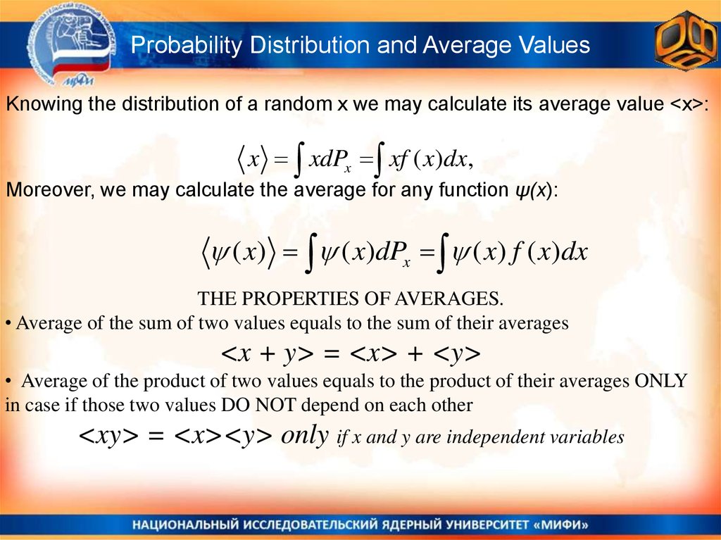
Probability Distribution and Average Values
Knowing the distribution of a random x we may calculate its average value <x>:
x xdPx xf ( x)dx,
Moreover, we may calculate the average for any function ψ(x):
( x) ( x)dPx ( x) f ( x)dx
THE PROPERTIES OF AVERAGES.
• Average of the sum of two values equals to the sum of their averages
<x + y> = <x> + <y>
• Average of the product of two values equals to the product of their averages ONLY
in case if those two values DO NOT depend on each other
<xy> = <x><y> only if x and y are independent variables

12.

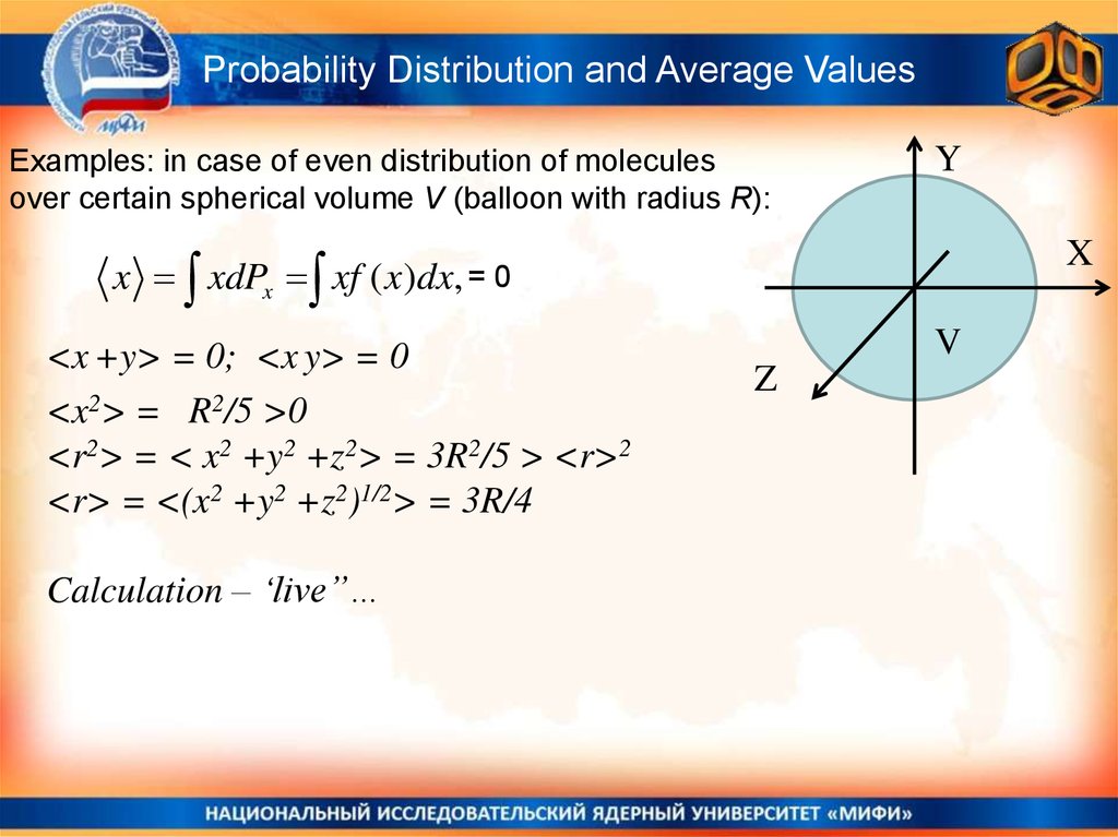
Probability Distribution and Average Values
Examples: in case of even distribution of molecules
over certain spherical volume V (balloon with radius R):
Y
X
x xdPx xf ( x)dx, = 0
<x +y> = 0; <x y> = 0
<x2> = R2/5 >0
<r2> = < x2 +y2 +z2> = 3R2/5 > <r>2
<r> = <(x2 +y2 +z2)1/2> = 3R/4
Calculation – ‘live”…
V
Z

13.

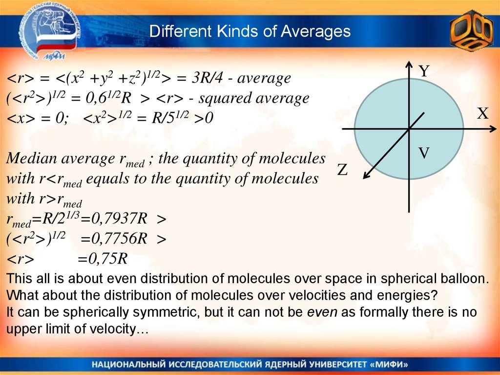
Different Kinds of Averages
<r> = <(x2 +y2 +z2)1/2> = 3R/4 - average
(<r2>)1/2 = 0,61/2R > <r> - squared average
<x> = 0; <x2>1/2 = R/51/2 >0
Y
Median average rmed ; the quantity of molecules
with r<rmed equals to the quantity of molecules Z
with r>rmed
rmed=R/21/3=0,7937R >
(<r2>)1/2 =0,7756R >
<r>
=0,75R
V
X
This all is about even distribution of molecules over space in spherical balloon.
What about the distribution of molecules over velocities and energies?
It can be spherically symmetric, but it can not be even as formally there is no
upper limit of velocity…

14.

Normal Distribution
Eagle and Tails game

15.

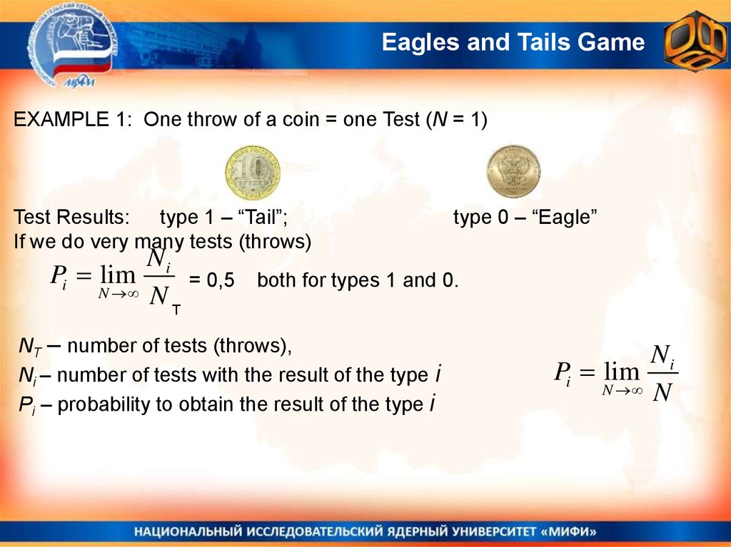
Eagles and Tails Game
EXAMPLE 1: One throw of a coin = one Test (N = 1)
Test Results: type 1 – “Tail”;
If we do very many tests (throws)
Ni
Pi lim
N N
T
= 0,5
type 0 – “Eagle”
both for types 1 and 0.
NT – number of tests (throws),
Ni – number of tests with the result of the type i
Рi – probability to obtain the result of the type i
Ni
Pi lim
N N

16.

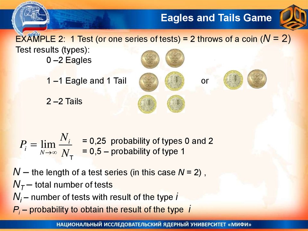
Eagles and Tails Game
EXAMPLE 2: 1 Test (or one series of tests) = 2 throws of a coin (N = 2)
Test results (types):
0 –2 Eagles
1 –1 Eagle and 1 Tail
or
2 –2 Tails
Ni
Pi lim
N N
T
= 0,25 probability of types 0 and 2
= 0,5 – probability of type 1
N – the length of a test series (in this case N = 2) ,
NT – total number of tests
Ni – number of tests with result of the type i
Рi – probability to obtain the result of the type i

17.

SOME MATHEMATICS
The product of probabilities:
The first test – the probability of result “1” - P1
The second test – the probability of result “2” = P2.
The probability to obtain the result ‘1’ at first attempt and then to obtain result
‘2’ at second attempt equals to the product of probabilities
P(1 AND 2) = P(1 ∩ 2) = P1P2
EXAMPLE: Eagle AND Tail = ½ * ½ = ¼
The SUM of probabilities:
One test – the probability of result “1” - P1; the probability of result “2” = P2.
The probability to obtain the result ‘1’ OR ‘2’ equals to the SUM of
probabilities: P(1TOR 2) = P(1 U 2) = P1 + P2
EXAMPLE: Eagle OR Tail = ½ + ½ = 1
EXAMPLE 2: (Eagle AND Tail) OR (Tail AND Eagle) = ¼ + ¼ = ½

18.

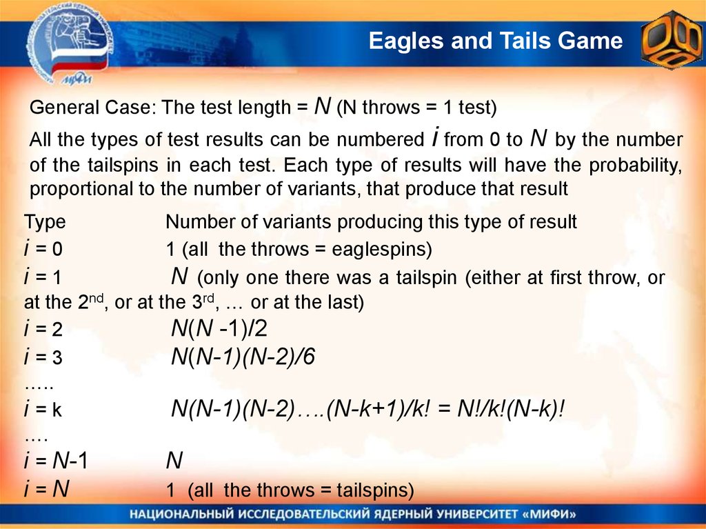
Eagles and Tails Game
General Case: The test length = N (N throws = 1 test)
All the types of test results can be numbered i from 0 to N by the number
of the tailspins in each test. Each type of results will have the probability,
proportional to the number of variants, that produce that result
Type
Number of variants producing this type of result
i=0
1 (all the throws = eaglespins)
i=1
N (only one there was a tailspin (either at first throw, or
at the 2nd, or at the 3rd, … or at the last)
i=2
N(N -1)/2
i=3
N(N-1)(N-2)/6
…..
i=k
N(N-1)(N-2)….(N-k+1)/k! = N!/k!(N-k)!
….
i = N-1
N
i=N
1 (all the throws = tailspins)

19.

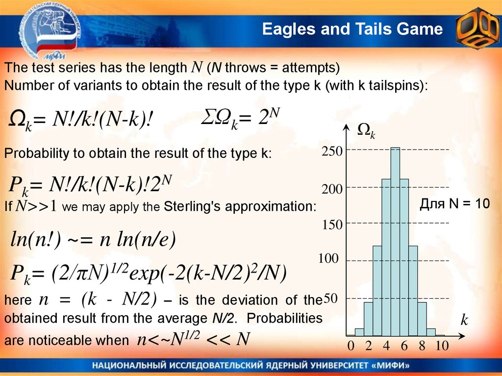
Eagles and Tails Game
The test series has the length N (N throws = attempts)
Number of variants to obtain the result of the type k (with k tailspins):
Ωk= N!/k!(N-k)!
ΣΩk= 2N
k
Probability to obtain the result of the type k:
250
Pk= N!/k!(N-k)!2N
200
If N>>1 we may apply the Sterling's approximation:
ln(n!) ~= n ln(n/e)
Pk= (2/πN)1/2exp(-2(k-N/2)2/N)
Для N = 10
150
100
here n = (k - N/2) – is the deviation of the 50
obtained result from the average N/2. Probabilities
are noticeable when
n<~N1/2 << N
k
0 2 4 6 8 10

20.

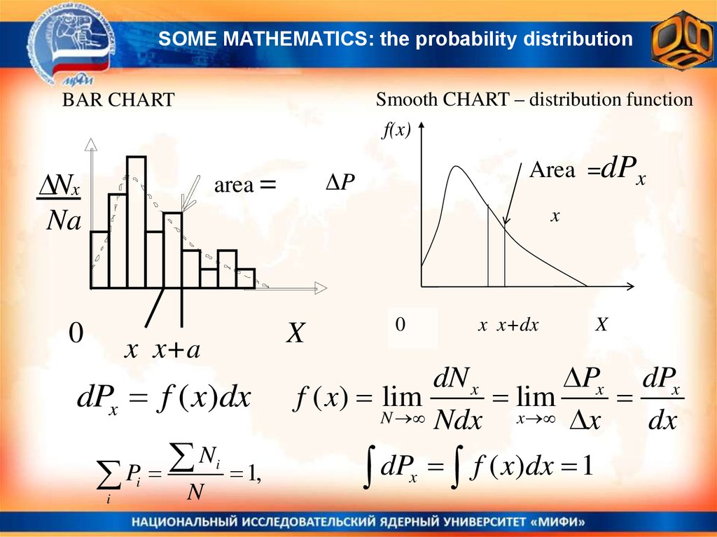
SOME MATHEMATICS: the probability distribution
Smooth CHART – distribution function
f(x)
BAR CHART
Nx
Na
Area =dPx
ΔP
area =
x
0
X
x x+a
dPx f ( x)dx
N
P
i
i
N
i
1,
0
x x+dx
X
dN x
Px dPx
f ( x) lim
lim
N Ndx
x x
dx
dP f ( x)dx 1
x

21.

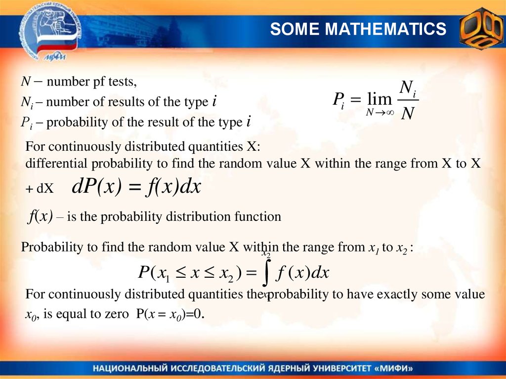
SOME MATHEMATICS
N – number pf tests,
Ni – number of results of the type i
Рi – probability of the result of the type i
Ni
Pi lim
N N
For continuously distributed quantities X:
differential probability to find the random value X within the range from X to X
+ dX
dP(x) = f(x)dx
f(x) – is the probability distribution function
Probability to find the random value X within
x2 the range from x1 to x2 :
P( x1 x x2 )
f ( x)dx
For continuously distributed quantities thex1probability to have exactly some value
x0, is equal to zero P(x = x0)=0.

22.

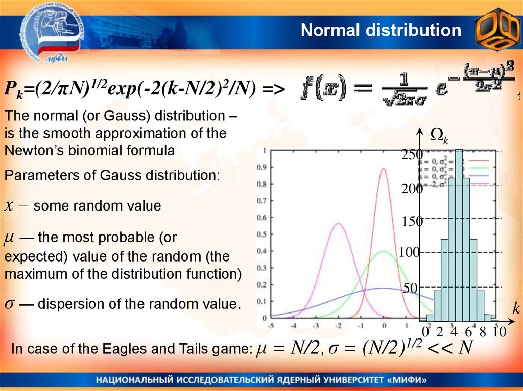
Normal distribution
Pk=(2/πN)1/2exp(-2(k-N/2)2/N) =>
The normal (or Gauss) distribution –
is the smooth approximation of the
Newton’s binomial formula
k
250
Parameters of Gauss distribution:
x – some random value
μ — the most probable (or
expected) value of the random (the
maximum of the distribution function)
σ — dispersion of the random value.
In case of the Eagles and Tails game: μ
200
150
100
50
k
0 2 4 6 8 10
= N/2, σ = (N/2)1/2 << N

23.

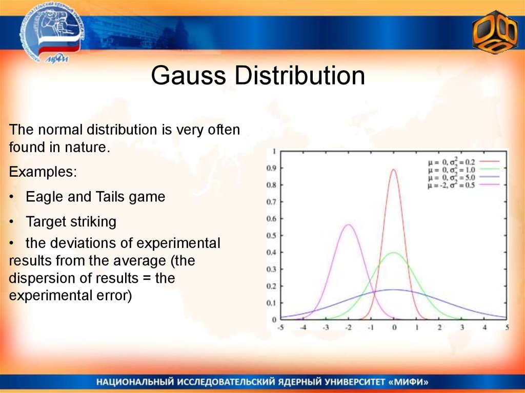
Gauss Distribution
The normal distribution is very often
found in nature.
Examples:
• Eagle and Tails game
• Target striking
• the deviations of experimental
results from the average (the
dispersion of results = the
experimental error)

24.

MEPhI General Physics
Normal (Gauss) Distribution
and Entropy

25.

Normal Distribution.
EXAMPLE: Eagles and Tails Game
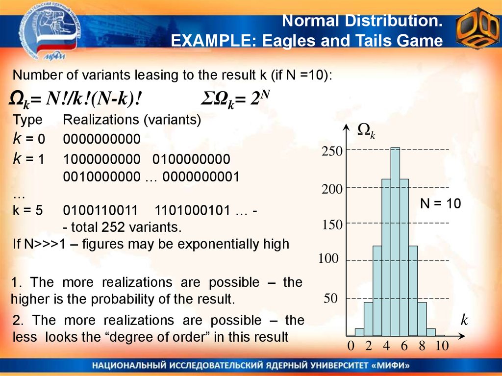
Number of variants leasing to the result k (if N =10):
Ωk= N!/k!(N-k)!
Type
k=0
k=1
ΣΩk= 2N
Realizations (variants)
0000000000
1000000000 0100000000
0010000000 … 0000000001
…
k=5
0100110011 1101000101 … - total 252 variants.
If N>>>1 – figures may be exponentially high
k
250
200
N = 10
150
100
1. The more realizations are possible – the
higher is the probability of the result.
2. The more realizations are possible – the
less looks the “degree of order” in this result
50
k
0 2 4 6 8 10

26.

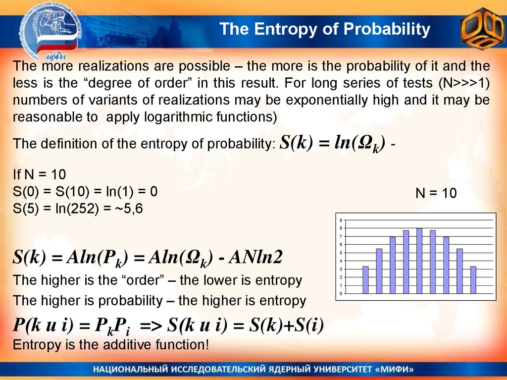
The Entropy of Probability
The more realizations are possible – the more is the probability of it and the
less is the “degree of order” in this result. For long series of tests (N>>>1)
numbers of variants of realizations may be exponentially high and it may be
reasonable to apply logarithmic functions)
The definition of the entropy of probability: S(k)
= ln(Ωk) -
If N = 10
S(0) = S(10) = ln(1) = 0
S(5) = ln(252) = ~5,6
N = 10
9
8
7
6
S(k) = Aln(Pk) = Aln(Ωk) - ANln2
The higher is the “order” – the lower is entropy
The higher is probability – the higher is entropy
P(k и i) = PkPi => S(k и i) = S(k)+S(i)
Entropy is the additive function!
5
4
3
2
1
0

27.

Entropy in Informatics
Type of result
k=0
k=1
k=5
Realizations
0000000000
1000000000 0100000000 ...
0100110011 1101000101 …
Any information or communication can be coded as a string of zeroes and
units: 0110010101110010010101111110001010111…. (binary code)
To any binary code with length N (consisting of N digits, k of which are
units and (N-k) – are zeroes) we may assign a value of entropy:
S(N,k) = ln(ΩN,k), where ΩN,k – is the number of variants how we may
compose a string out of k units and (N-k) zeroes
• Communications, looking like 00000000.. 111111111… S = 0
• Communications with equal number of units and zeroes have maximal
entropy .
• Entropy of 2 communications equals to the sum of their entropies.

28.

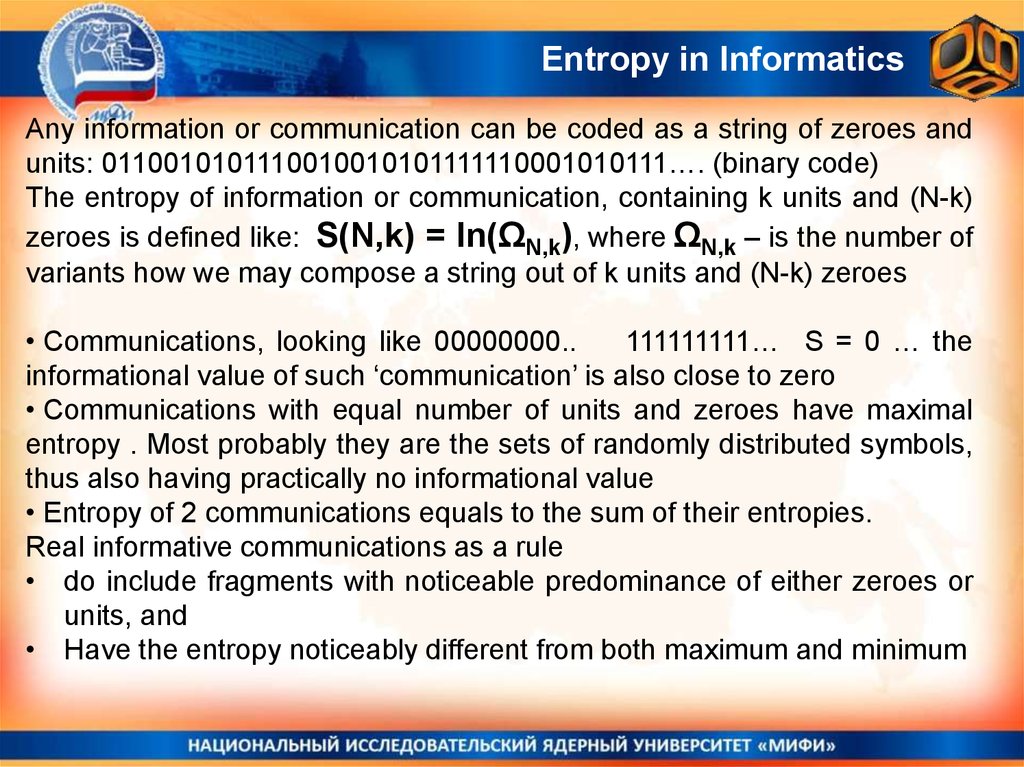
Entropy in Informatics
Any information or communication can be coded as a string of zeroes and
units: 0110010101110010010101111110001010111…. (binary code)
The entropy of information or communication, containing k units and (N-k)
zeroes is defined like: S(N,k) = ln(ΩN,k), where ΩN,k – is the number of
variants how we may compose a string out of k units and (N-k) zeroes
• Communications, looking like 00000000..
111111111… S = 0 … the
informational value of such ‘communication’ is also close to zero
• Communications with equal number of units and zeroes have maximal
entropy . Most probably they are the sets of randomly distributed symbols,
thus also having practically no informational value
• Entropy of 2 communications equals to the sum of their entropies.
Real informative communications as a rule
• do include fragments with noticeable predominance of either zeroes or
units, and
• Have the entropy noticeably different from both maximum and minimum

29.

Entropy in Informatics
The deffinition of entropy as the measure of
disorder (or the measure of informational
value) in informatics was first introduced by
Claude Shannon in his article «A
Mathematical Theory of Communication»,
published in Bell System Technical Journal
in 1948
Those ideas still serve as the base for the
theory of connunications, tmethods on
encoding and decoding, are used in
linguistics etc…
Claude Elwood Shannon
1916 - 2001

30.

MEPhI General Physics
Statistical Entropy in Physics

31.

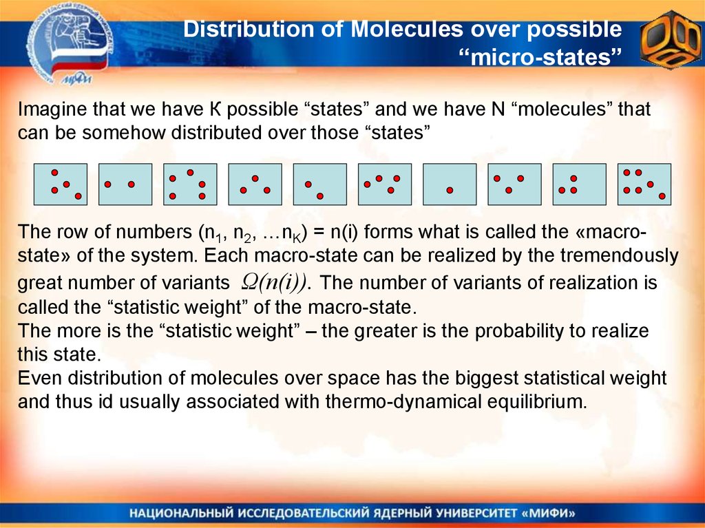
Distribution of Molecules over possible
“micro-states”
Imagine that we have К possible “states” and we have N “molecules” that
can be somehow distributed over those “states”
The row of numbers (n1, n2, …nK) = n(i) forms what is called the «macrostate» of the system. Each macro-state can be realized by the tremendously
great number of variants Ω(n(i)). The number of variants of realization is
called the “statistic weight” of the macro-state.
The more is the “statistic weight” – the greater is the probability to realize
this state.
Even distribution of molecules over space has the biggest statistical weight
and thus id usually associated with thermo-dynamical equilibrium.

32.

Statistical Entropy in Physics.
Statistical Entropy in Molecular Physics: the logarithm of the number of
possible micro-realizations of a state with certain macro-parameters,
multiplied by the Boltzmann constant.
S k ln J/K
1.
2.
3.
4.
5.
In the state of thermodynamic equilibrium, the entropy of a closed
system has the maximum possible value (for a given energy).
If the system (with the help of external influence)) is derived from the
equilibrium state - its entropy can become smaller. BUT…
If a nonequilibrium system is left to itself - it relaxes into an equilibrium
state and its entropy increases
The entropy of an isolated system for any processes does not
decrease, i.e. ΔS > 0 , as the spontaneous transitions from more
probable (less ordered) to less probable (more ordered) states in
molecular systems have negligibly low probability
The entropy is the measure of disorder in molecular systems.

33.

Statistical Entropy in Physics.
For the state of the molecular system with certain macroscopic parameters
we may introduce the definition of Statistical Entropy as the logarithm of the
number of possible micro-realizations (the statistical weight of a state Ώ) of a this state, multiplied by the Boltzmann constant.
S k ln J/К
Entropy is the additive quantity.
2
1
i
3
p p1 p2 ... pN
pi
i
1 2 ... N
N
S k ln k ln 1 ln 2 ... ln N
S Si
i 1

34.

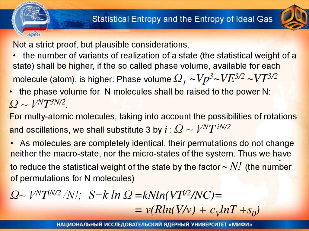
Statistical Entropy and the Entropy of Ideal Gas
Not a strict proof, but plausible considerations.
• the number of variants of realization of a state (the statistical weight of a
state) shall be higher, if the so called phase volume, available for each
molecule (atom), is higher: Phase volume Ω1 ~Vp3~VE3/2 ~VT3/2
• the phase volume for N molecules shall be raised to the power N:
Ω ~ VNT3N/2.
For multy-atomic molecules, taking into account the possibilities of rotations
and oscillations, we shall substitute 3 by i : Ω
~ VNT iN/2
• As molecules are completely identical, their permutations do not change
neither the macro-state, nor the micro-states of the system. Thus we have
to reduce the statistical weight of the state by the factor ~ N! (the number
of permutations for N molecules)
Ω~ VNTiN/2 /N!; S=k ln Ω =kNln(VTi/2/NC)=
= v(Rln(V/v) + cVlnT +s0)

35.

Statistical Entropy and the Entropy of Ideal Gas
Ω~ VNTiN/2 /N!; S=k ln Ω =kNln(VTi/2/NC)=
= v(Rln(V/v) + cVlnT +s0)
The statistical entropy proves to be the same physical quantity, as was
earlier defined in thermodynamics without even referring to the molecular
structure of matter and heat!

36.

2nd Law of Thermodynamics and the ‘Time arrow’
“The increase of disorder, or the
increase of the Entropy, of the
Universe over time is one of the possibilities to define the
so-called “Time arrow”, that is the
direction of time, or the ability to
distinguish the past from the future,
Stephen Hawking
(1942-2018)

37.

MEPhI General Physics
The Distributions of Molecules
over Velocities and Energies
Maxwell and Boltzmann Distributions
That will be the Focus of the next lecture!

38.

Thank You for Attention!

English Русский Rules