541.37K

Category: $mathematics$ mathematics

Normal Probability Distributions

1.

Chapter 6
Normal Probability Distributions
The Standard Normal Distribution
Applications of Normal Distributions
The Central Limit Theorem
Normal as Approximation to Binomial
Copyright © 2010, 2007, 2004 Pearson Education, Inc.
6.1 - 1

2.

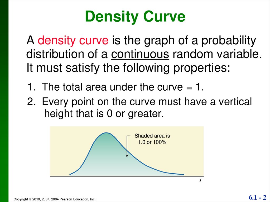
Density Curve
A density curve is the graph of a probability
distribution of a continuous random variable.
It must satisfy the following properties:
1. The total area under the curve = 1.
2. Every point on the curve must have a vertical
height that is 0 or greater.
Shaded area is
1.0 or 100%
x
Copyright © 2010, 2007, 2004 Pearson Education, Inc.
6.1 - 2

3.

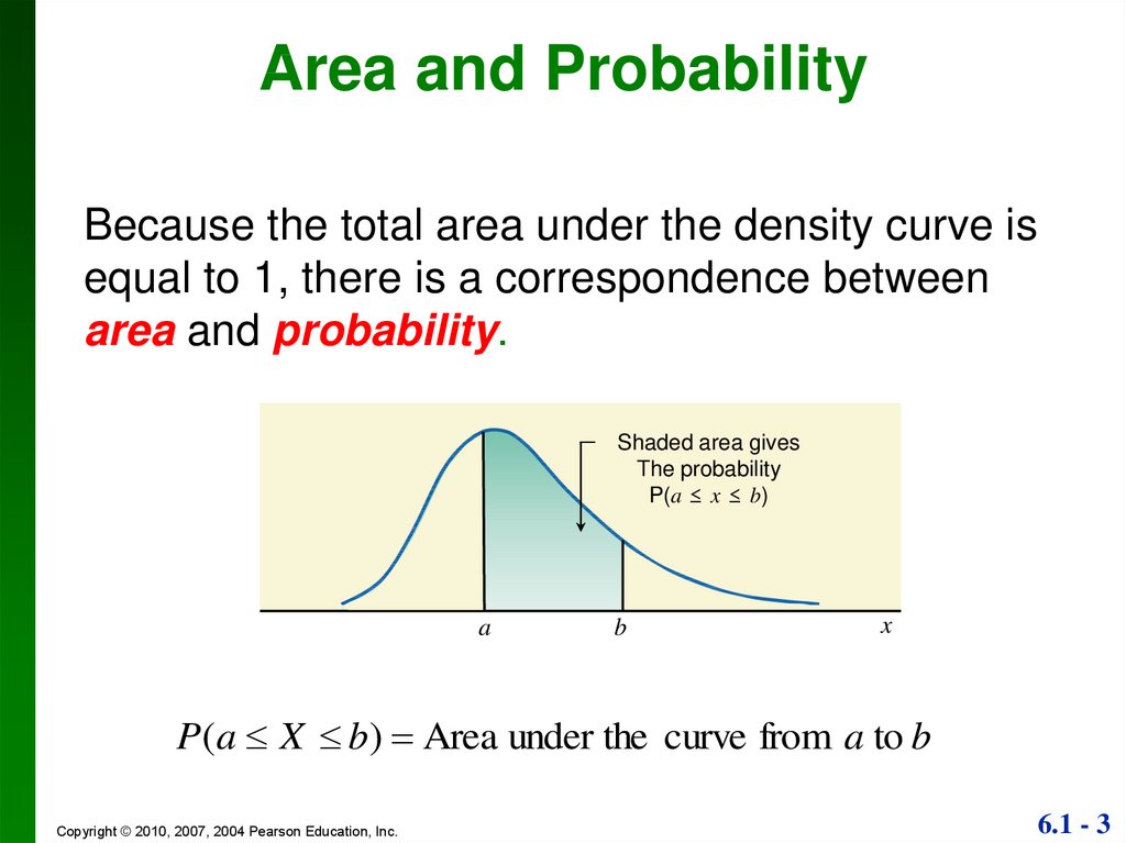
Area and Probability
Because the total area under the density curve is
equal to 1, there is a correspondence between
area and probability.
Shaded area gives
The probability
P(a ≤ x ≤ b)
a
b
x
P(a X b) Area under the curve from a to b
Copyright © 2010, 2007, 2004 Pearson Education, Inc.
6.1 - 3

4.

Uniform Distribution
(Definition) A continuous random variable has a
uniform distribution if its values are spread evenly
over the given range of an interval.
Note : the graph of a uniform distribution results in a
rectangular shape.
Copyright © 2010, 2007, 2004 Pearson Education, Inc.
6.1 - 4

5.

(Example) A power company provides electricity
with voltage levels between 123.0 volts and 125.0
volts, and all of the possible values are equally
likely. Then, the voltage levels are uniformly
distributed between 123.0 volts and 125.0 volts.
Find the probability that a randomly selected voltage
level is greater than 124.5 volts.
P(x)
0.5
0
123.0 123.5
Area = 0.5 x 0.5
= 0.25
124 124.5 125.0
Voltage
Copyright © 2010, 2007, 2004 Pearson Education, Inc.
x
6.1 - 5

6.

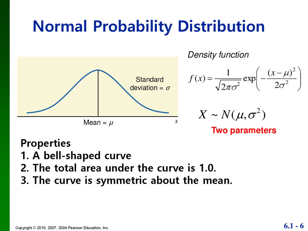
Normal Probability Distribution
Density function
( x )2
f ( x)
exp
2
2
2
2
1
Standard
deviation = σ
X ~ N ( , )
2
Mean = μ
x
Two parameters
Properties
1. A bell-shaped curve
2. The total area under the curve is 1.0.
3. The curve is symmetric about the mean.
Copyright © 2010, 2007, 2004 Pearson Education, Inc.
6.1 - 6

7.

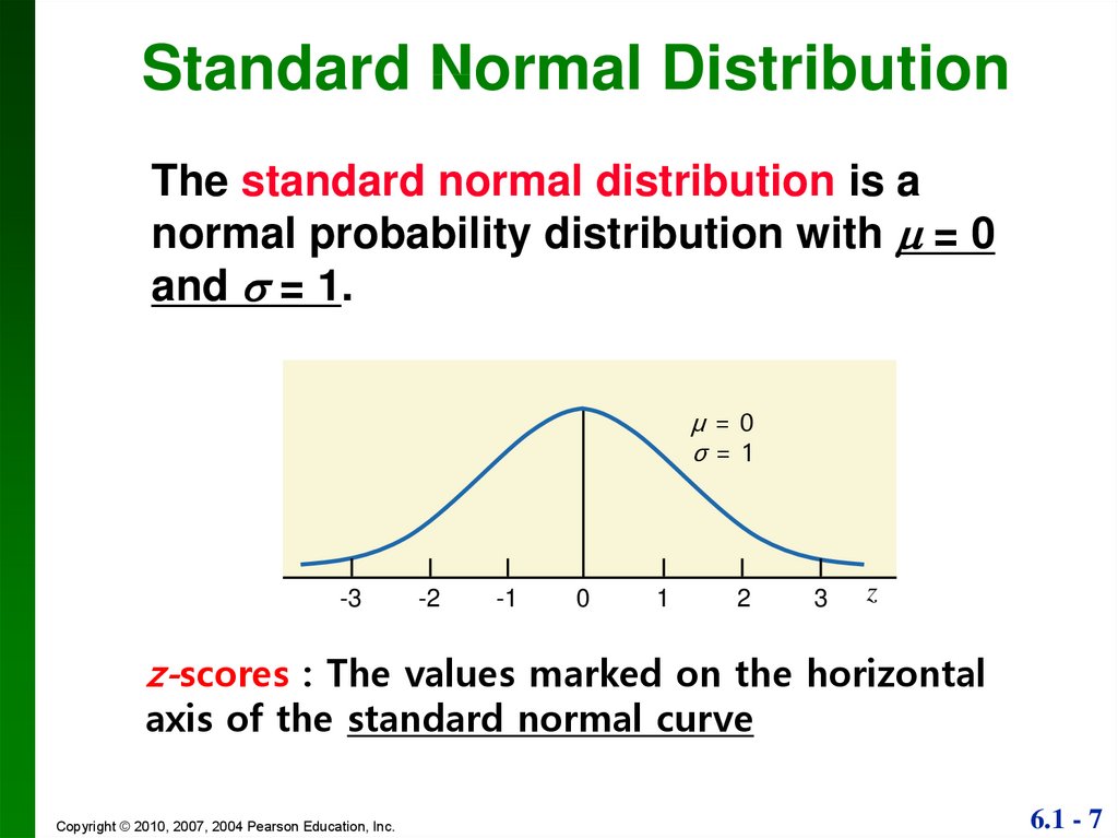
Standard Normal Distribution
The standard normal distribution is a
normal probability distribution with = 0
and = 1.
μ=0
σ=1
-3
-2
-1
0
1
2
3
z
z-scores : The values marked on the horizontal
axis of the standard normal curve
Copyright © 2010, 2007, 2004 Pearson Education, Inc.
6.1 - 7

8.

Finding probability
when z-scores are given
P(a < Z < b) = probability that the z-score is between a
and b.
P(Z > a) = probability that the z-score is greater than a.
P(Z < a) = probability that the z-score is less than a.
To find the above probabilities,
we can use R, Excel or Statistical Table
Copyright © 2010, 2007, 2004 Pearson Education, Inc.
6.1 - 8

9.

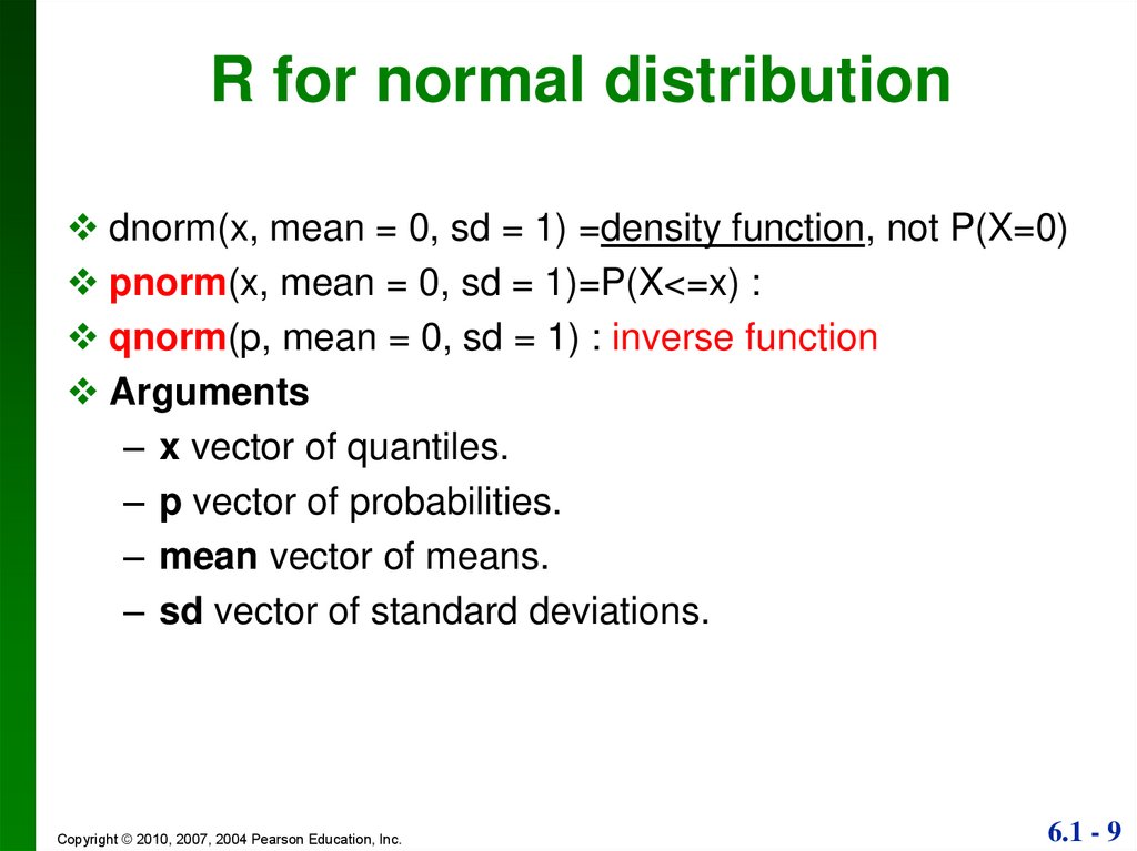
R for normal distribution
dnorm(x, mean = 0, sd = 1) =density function, not P(X=0)
pnorm(x, mean = 0, sd = 1)=P(X<=x) :
qnorm(p, mean = 0, sd = 1) : inverse function
Arguments
– x vector of quantiles.
– p vector of probabilities.
– mean vector of means.
– sd vector of standard deviations.
Copyright © 2010, 2007, 2004 Pearson Education, Inc.
6.1 - 9

10.

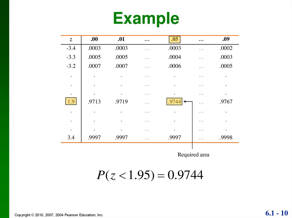
Example
z
.00
.01
…
.05
…
.09
-3.4
.0003
.0003
…
.0003
…
.0002
-3.3
.0005
.0005
…
.0004
…
.0003
-3.2
.0007
.0007
…
.0006
…
.0005
.
.
.
…
.
…
.
.
.
.
…
.
…
.
.
.
.
…
.
…
.
1.9
.9713
.9719
…
.9744
…
.9767
.
.
.
…
.
…
.
.
.
.
…
.
…
.
.
.
.
…
.
…
.
3.4
.9997
.9997
…
.9997
…
.9998
Required area
P( z 1.95) 0.9744
Copyright © 2010, 2007, 2004 Pearson Education, Inc.
6.1 - 10

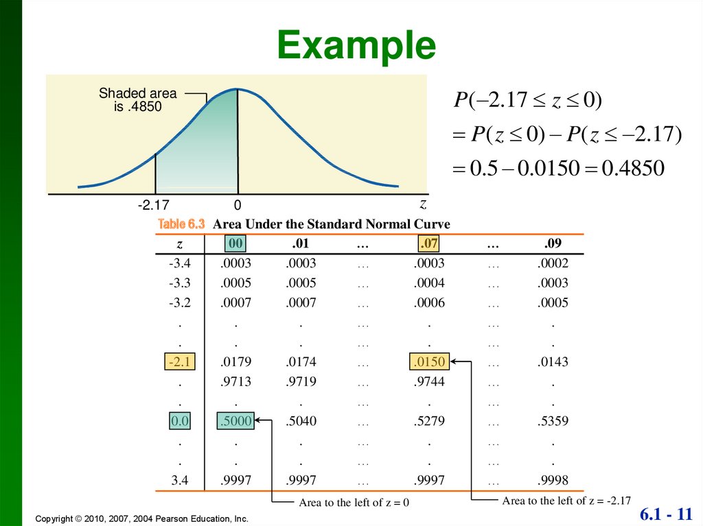
11.

Example
P( 2.17 z 0)
P( z 0) P( z 2.17)
Shaded area
is .4850
0.5 0.0150 0.4850
z
-2.17
0
Table 6.3 Area Under the Standard Normal Curve
z
00
.01
…
.07
-3.4
.0003
.0003
…
.0003
-3.3
.0005
.0005
…
.0004
-3.2
.0007
.0007
…
.0006
.
.
.
…
.
.
.
.
…
.
-2.1
.0179
.0174
…
.0150
.
.9713
.9719
…
.9744
.
.
.
…
.
0.0
.5000
.5040
…
.5279
.
.
.
…
.
.
.
.
…
.
3.4
.9997
.9997
…
.9997
Area to the left of z = 0
Copyright © 2010, 2007, 2004 Pearson Education, Inc.
…
…
…
…
…
…
…
…
…
…
…
…
…
.09
.0002
.0003
.0005
.
.
.0143
.
.
.5359
.
.
.9998
Area to the left of z = -2.17
6.1 - 11

12.

Example I
Assume that the readings of a thermometer are normally
distributed with the mean 0ºC and the standard deviation
1.00ºC. If one thermometer is randomly selected,
find the probability that, at the freezing point of water (0º),
the reading is less than 1.27º.
pnorm(1.27,0,1)
Copyright © 2010, 2007, 2004 Pearson Education, Inc.
6.1 - 12

13.

Example I
P(Z < 1.27) = ??
TABLE A-2
(Continued) Cumulative Area from the LEFT
z
.00
.01
.02
.03
.04
.05
.06
.07
0.0
.5000
.5040
.5080
.5120
.5160
.5199
.5239
.5279
0.1
.5398
.5438
.5478
.5517
.5557
.5596
.5636
.5675
0.2
.5793
.5382
.5871
.5910
.5948
.5987
.6026
.6064
1.0
.8413
.8438
.8461
.8485
.8508
.8531
.8554
.8577
1.1
.8643
.8665
.8686
.8708
.8729
.8749
.8770
.8790
1.2
.8849
.8869
.8888
.8907
.8925
.8944
.8962
.8980
1.3
.9032
.9049
.9066
.9082
.9099
.9115
.9131
.9147
1.4
.9192
.9207
.9222
.9236
.9251
.9265
.9279
.9292
Copyright © 2010, 2007, 2004 Pearson Education, Inc.
P (Z < 1.27) = 0.8980
The probability of randomly
selecting a thermometer with
a reading less than 1.27º is
0.8980.
6.1 - 13

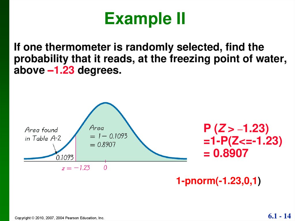
14.

Example II
If one thermometer is randomly selected, find the
probability that it reads, at the freezing point of water,
above –1.23 degrees.
P (Z > –1.23)
=1-P(Z<=-1.23)
= 0.8907
1-pnorm(-1.23,0,1)
Copyright © 2010, 2007, 2004 Pearson Education, Inc.
6.1 - 14

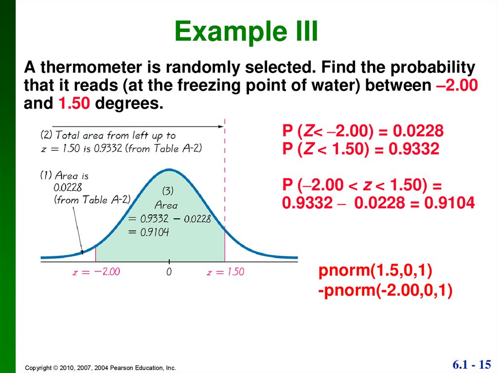
15.

Example III
A thermometer is randomly selected. Find the probability
that it reads (at the freezing point of water) between –2.00
and 1.50 degrees.
P (Z< –2.00) = 0.0228
P (Z < 1.50) = 0.9332
P (–2.00 < z < 1.50) =
0.9332 – 0.0228 = 0.9104
pnorm(1.5,0,1)
-pnorm(-2.00,0,1)
Copyright © 2010, 2007, 2004 Pearson Education, Inc.
6.1 - 15

16.

Finding z Scores
When Given Probabilities
– Inverse problem
5% or 0.05
Finding the 95th Percentile
qnorm(0.95, mean = 0, sd = 1)=1.645
Copyright © 2010, 2007, 2004 Pearson Education, Inc.
6.1 - 16

17.

Applications of Normal
Distributions
Copyright © 2010, 2007, 2004 Pearson Education, Inc.
6.1 - 17

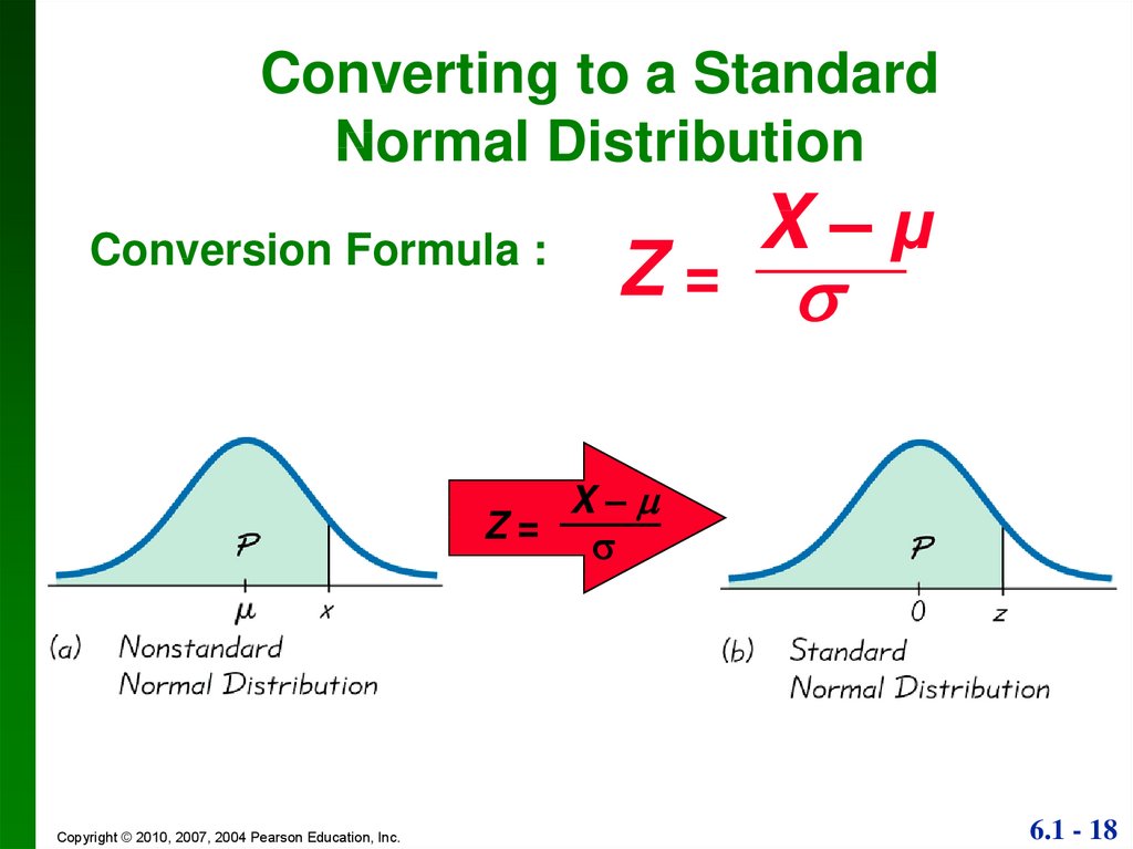
18.

Converting to a Standard
Normal Distribution
Conversion Formula :
X–µ
Z=
X–
Z=
Copyright © 2010, 2007, 2004 Pearson Education, Inc.
6.1 - 18

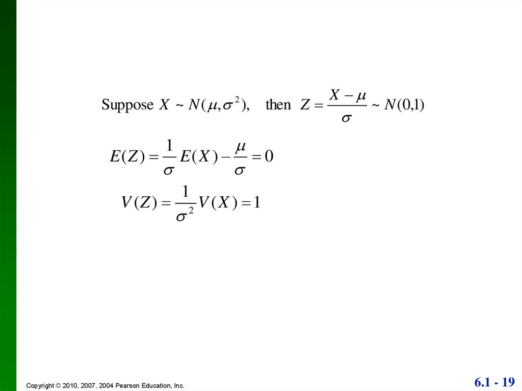
19.

Suppose X ~ N ( , 2 ), then Z
E (Z )
1
V (Z )
E( X )
1
Copyright © 2010, 2007, 2004 Pearson Education, Inc.
2
X
~ N (0,1)
0
V (X ) 1
6.1 - 19

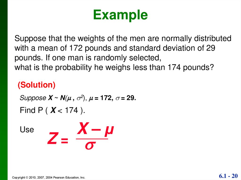
20.

Example
Suppose that the weights of the men are normally distributed
with a mean of 172 pounds and standard deviation of 29
pounds. If one man is randomly selected,
what is the probability he weighs less than 174 pounds?
(Solution)
Suppose X ~ N( , 2), = 172, = 29.
Find P ( X < 174 ).
Use
X–µ
Z=
Copyright © 2010, 2007, 2004 Pearson Education, Inc.
6.1 - 20

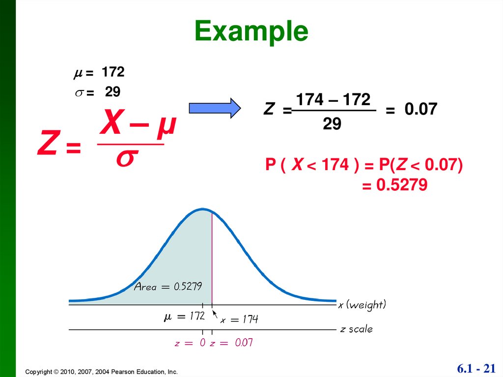
21.

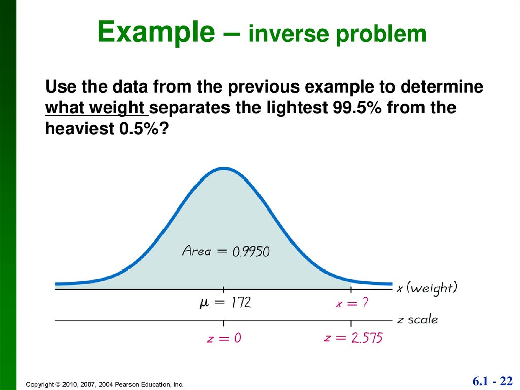
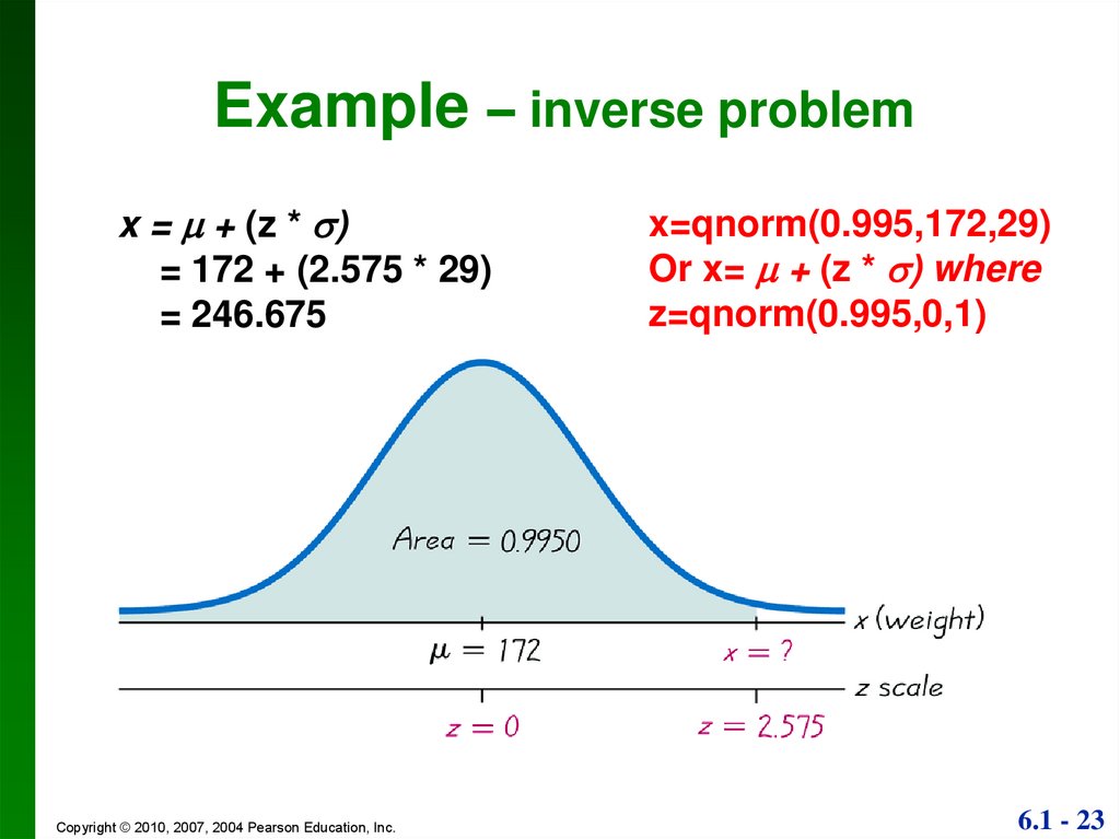
22.

Example – inverse problem
Use the data from the previous example to determine
what weight separates the lightest 99.5% from the
heaviest 0.5%?
Copyright © 2010, 2007, 2004 Pearson Education, Inc.
6.1 - 22

23.

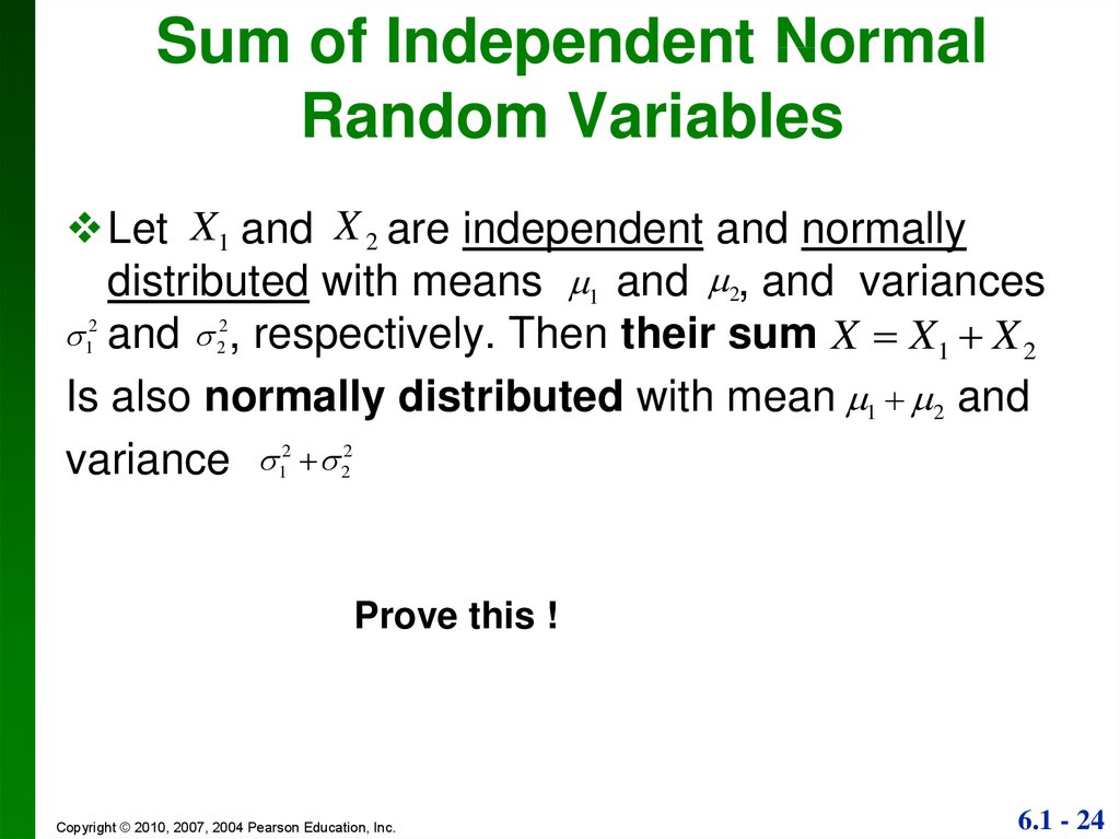
24.

Sum of Independent Normal
Random Variables
Let X1 and X 2 are independent and normally
distributed with means 1 and 2, and variances
12 and 22 , respectively. Then their sum X X1 X 2
Is also normally distributed with mean 1 2 and
variance 12 22
Prove this !
Copyright © 2010, 2007, 2004 Pearson Education, Inc.
6.1 - 24

25.

26.

Key Concept
The Central Limit Theorem tells us that for a
population with any distribution, the
distribution of the sample means approaches
a normal distribution as the sample size
increases.
The procedure in this section form the
foundation for estimating population
parameters and hypothesis testing.
Copyright © 2010, 2007, 2004 Pearson Education, Inc.
6.1 - 26

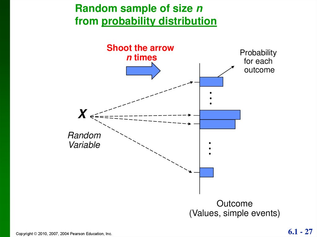
27.

Random sample of size n
from probability distribution
Shoot the arrow
n times
Probability
for each
outcome
X
Random
Variable
Outcome
(Values, simple events)
Copyright © 2010, 2007, 2004 Pearson Education, Inc.
6.1 - 27

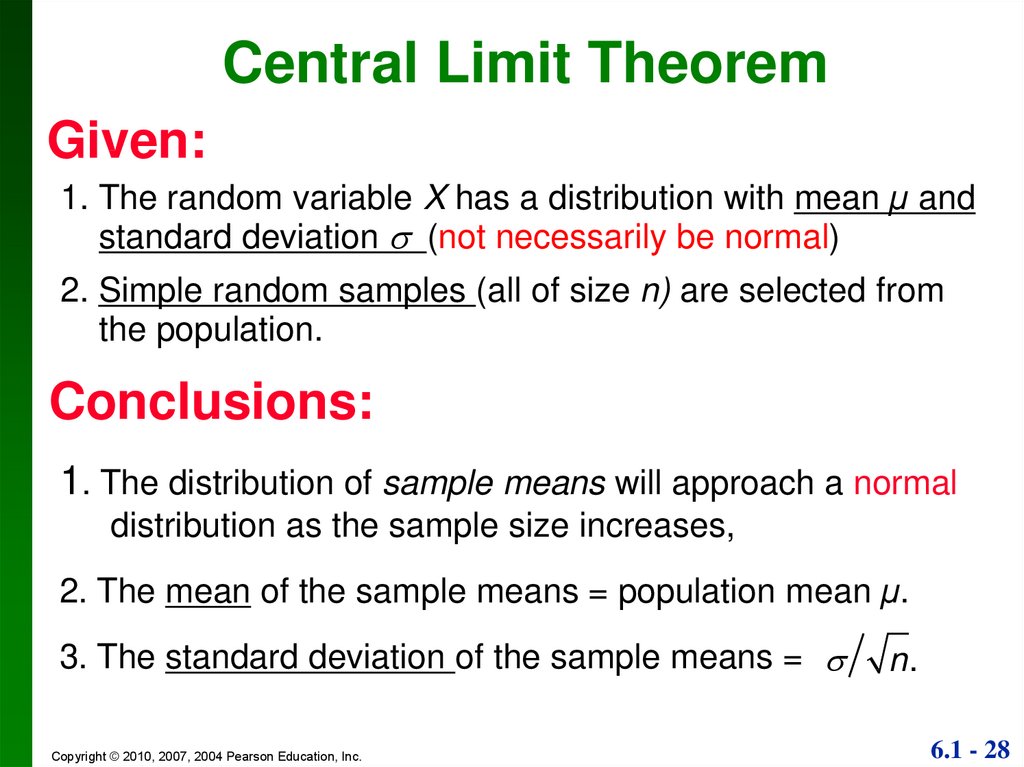
28.

Central Limit Theorem
Given:
1. The random variable X has a distribution with mean µ and
standard deviation (not necessarily be normal)
2. Simple random samples (all of size n) are selected from
the population.
Conclusions:
1. The distribution of sample means will approach a normal
distribution as the sample size increases,
2. The mean of the sample means = population mean µ.
3. The standard deviation of the sample means =
Copyright © 2010, 2007, 2004 Pearson Education, Inc.
n.
6.1 - 28

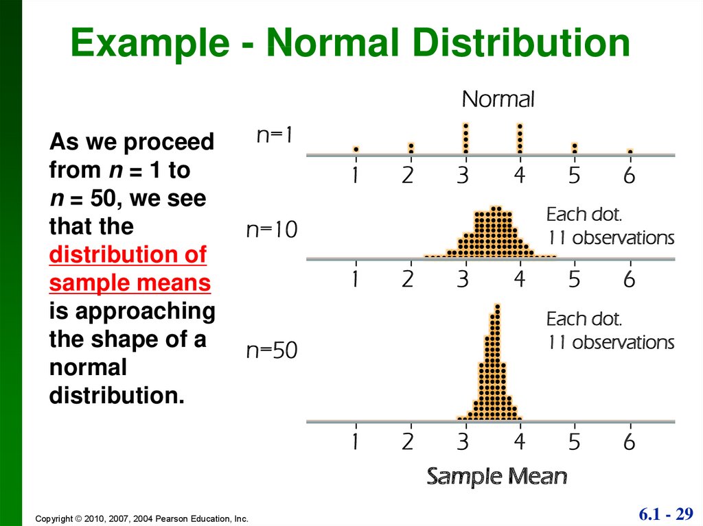
29.

Example - Normal Distribution
Normal
As we proceed
from n = 1 to
n = 50, we see
that the
distribution of
sample means
is approaching
the shape of a
normal
distribution.
n=1
1
2
3
4
6
Each dot.
11 observations
n=10
1
2
3
4
5
6
Each dot.
11 observations
n=50
1
Copyright © 2010, 2007, 2004 Pearson Education, Inc.
5
2
3
4
5
Sample Mean
6
6.1 - 29

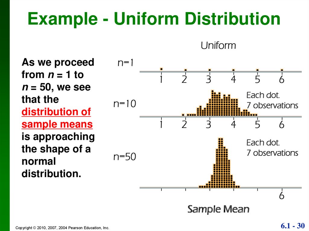
30.

Example - Uniform Distribution
Uniform
As we proceed
from n = 1 to
n = 50, we see
that the
distribution of
sample means
is approaching
the shape of a
normal
distribution.
n=1
1
2
3
4
6
Each dot.
7 observations
n=10
1
n=50
5
2
3
4
5
6
Each dot.
7 observations
6
Sample Mean
Copyright © 2010, 2007, 2004 Pearson Education, Inc.
6.1 - 30

31.

Example - U-Shaped Distribution
U-Shape
As we proceed
from n = 1 to
n = 50, we see
that the
distribution of
sample means
is approaching
the shape of a
normal
distribution.
n=1
1
3
4
5
6
Each dot.
7 observations
n=10
1
2
3
4
5
6
Each dot.
7 observations
n=50
1
Copyright © 2010, 2007, 2004 Pearson Education, Inc.
2
2
3
4
5
Sample Mean
6
6.1 - 31

32.

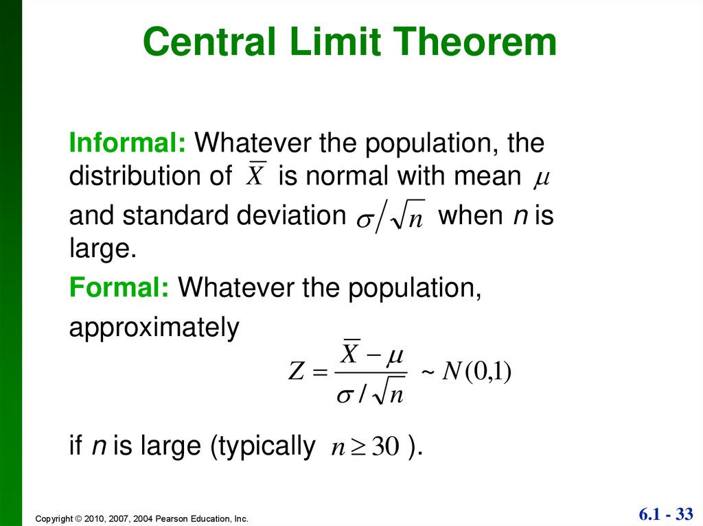
33.

Central Limit Theorem
Informal: Whatever the population, the
distribution of X is normal with mean
and standard deviation n when n is
large.
Formal: Whatever the population,
approximately
X
Z
~ N (0,1)
/ n
if n is large (typically n 30 ).
Copyright © 2010, 2007, 2004 Pearson Education, Inc.
6.1 - 33

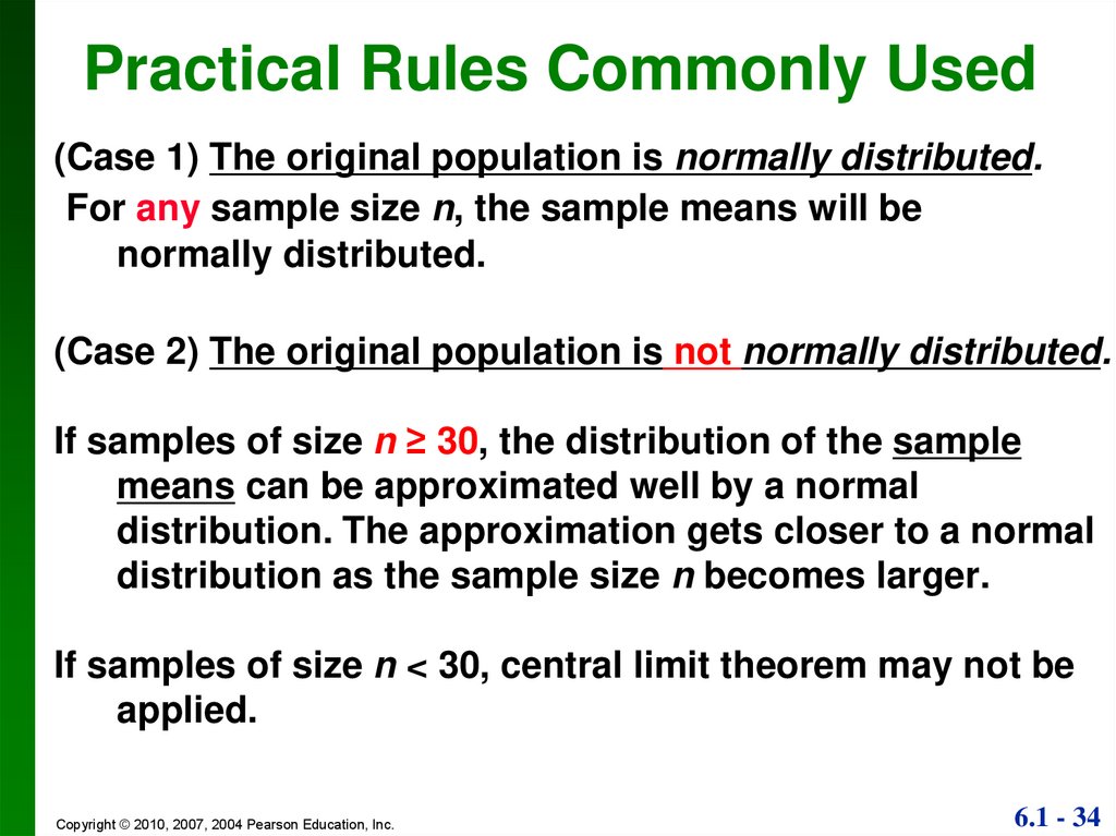
34.

Practical Rules Commonly Used
(Case 1) The original population is normally distributed.
For any sample size n, the sample means will be
normally distributed.
(Case 2) The original population is not normally distributed.
If samples of size n ≥ 30, the distribution of the sample
means can be approximated well by a normal
distribution. The approximation gets closer to a normal
distribution as the sample size n becomes larger.
If samples of size n < 30, central limit theorem may not be
applied.
Copyright © 2010, 2007, 2004 Pearson Education, Inc.
6.1 - 34

35.

Example
Assume the population of weights of men is
normally distributed with a mean of 172 lb and
a standard deviation of 29 lb.
a) Find the probability that if an individual man is
randomly selected, his weight is greater than 175 lb.
b) Find the probability that 20 randomly selected men
will have a mean weight that is greater than 175 lb
(so that their total weight exceeds the safe capacity
of 3500 pounds).
Copyright © 2010, 2007, 2004 Pearson Education, Inc.
6.1 - 35

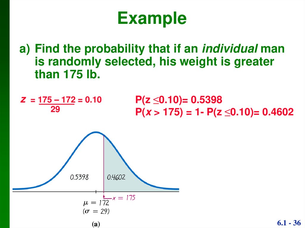
36.

Example
a) Find the probability that if an individual man
is randomly selected, his weight is greater
than 175 lb.
z = 175 – 172 = 0.10
29
Copyright © 2010, 2007, 2004 Pearson Education, Inc.
P(z ≤0.10)= 0.5398
P(x > 175) = 1- P(z ≤0.10)= 0.4602
6.1 - 36

37.

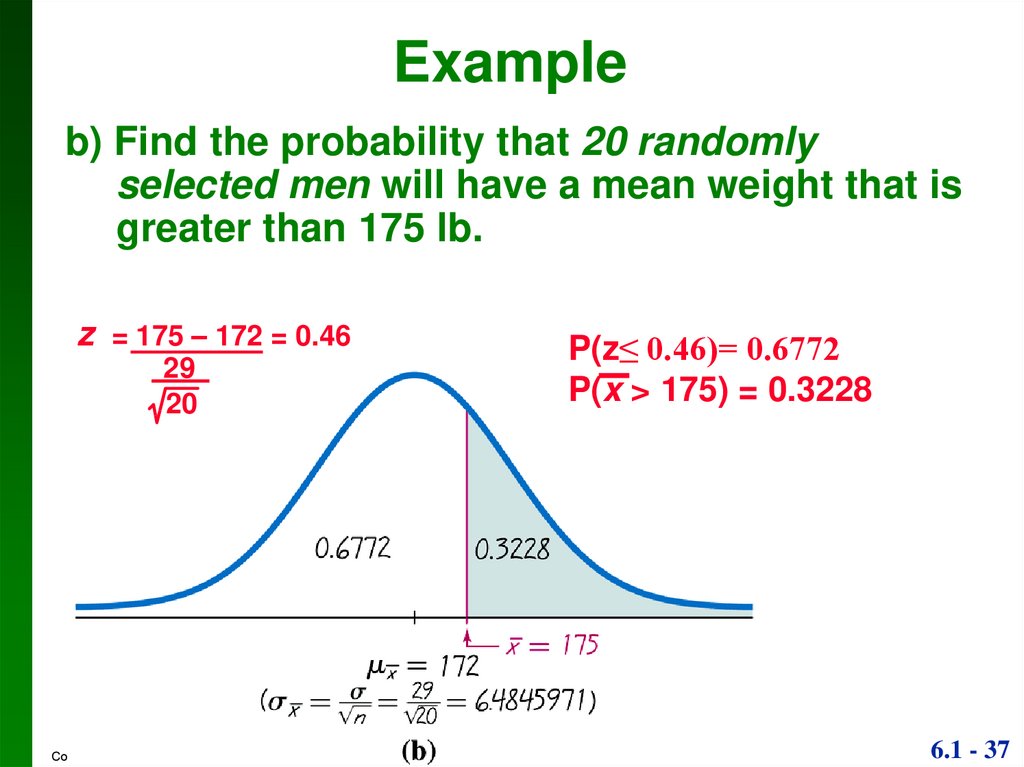
Example
b) Find the probability that 20 randomly
selected men will have a mean weight that is
greater than 175 lb.
z = 175 – 172 = 0.46
29
20
Copyright © 2010, 2007, 2004 Pearson Education, Inc.
P(z≤ 0.46)= 0.6772
P(x > 175) = 0.3228
6.1 - 37

38.

Example
Assume the population of weights of men has a
mean of 172 lb and a standard deviation of 29 lb
(not necessarily be normal). Find the probability
that 30 randomly selected men will have a mean
weight that is greater than 175 lb.
Copyright © 2010, 2007, 2004 Pearson Education, Inc.
6.1 - 38

39.

40.

Review
Binomial Probability Distribution
1. The procedure must have a fixed number of trials.
2. The trials must be independent.
3. Each trial must have all outcomes classified into two
categories (commonly, success and failure).
4. The probability of success remains the same in all trials.
Copyright © 2010, 2007, 2004 Pearson Education, Inc.
6.1 - 40

41.

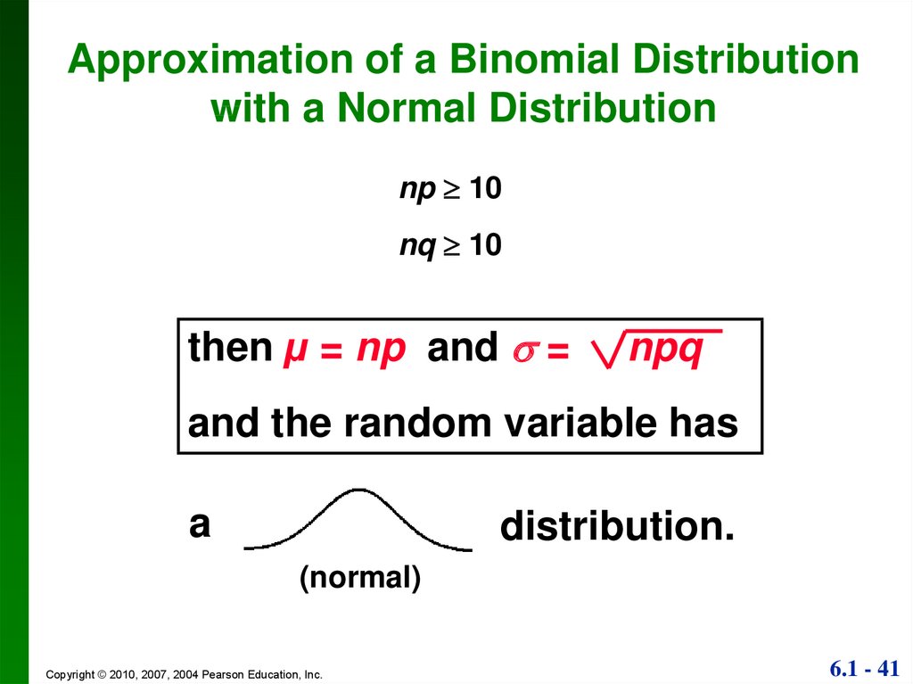
Approximation of a Binomial Distribution
with a Normal Distribution
np 10
nq 10
then µ = np and =
npq
and the random variable has
a
distribution.
(normal)
Copyright © 2010, 2007, 2004 Pearson Education, Inc.
6.1 - 41

42.

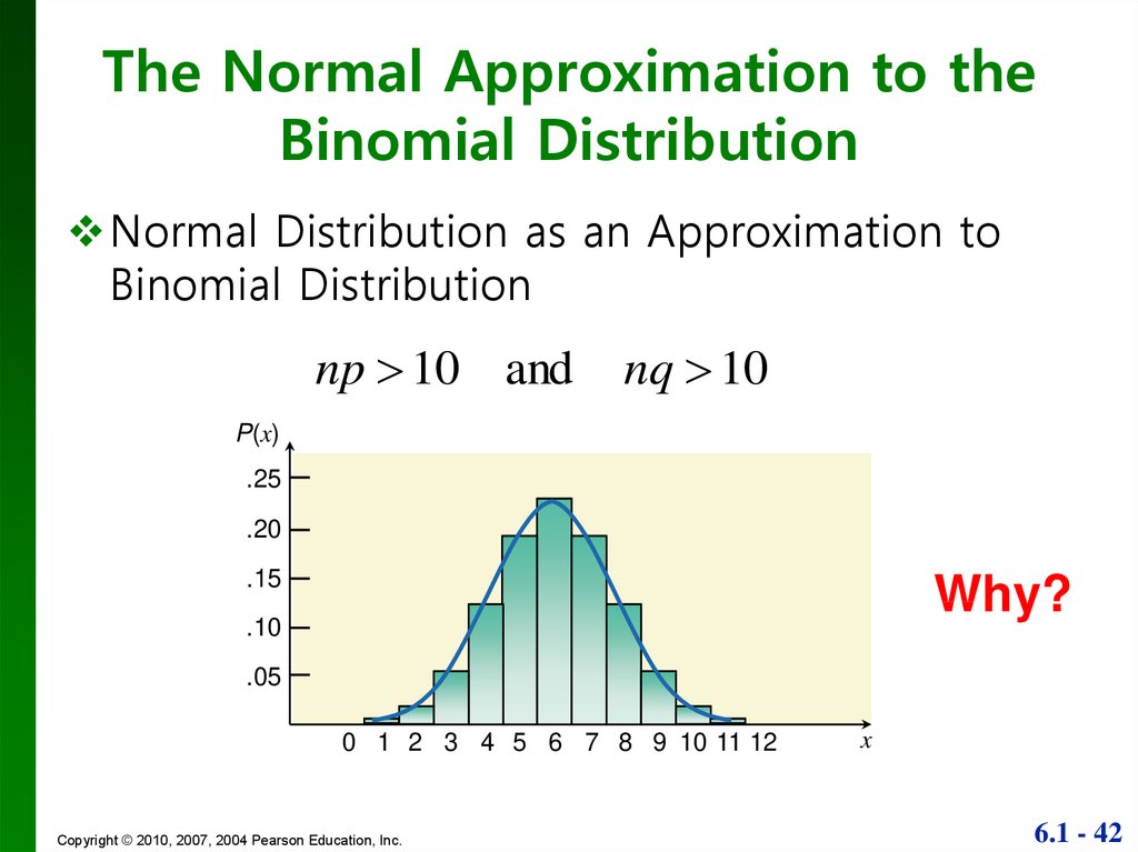
The Normal Approximation to the
Binomial Distribution
Normal Distribution as an Approximation to
Binomial Distribution
np 10 and
nq 10
P(x)
.25
.20
.15
Why?
.10
.05
0 1 2 3 4 5 6 7 8 9 10 11 12
Copyright © 2010, 2007, 2004 Pearson Education, Inc.
x
6.1 - 42

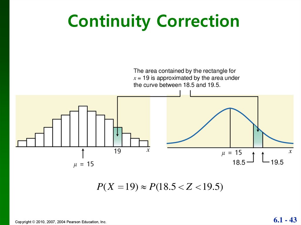
43.

Continuity Correction
The area contained by the rectangle for
x = 19 is approximated by the area under
the curve between 18.5 and 19.5.
19
μ = 15
x
μ = 15
18.5
x
19.5
P( X 19) P(18.5 Z 19.5)
Copyright © 2010, 2007, 2004 Pearson Education, Inc.
6.1 - 43

44.

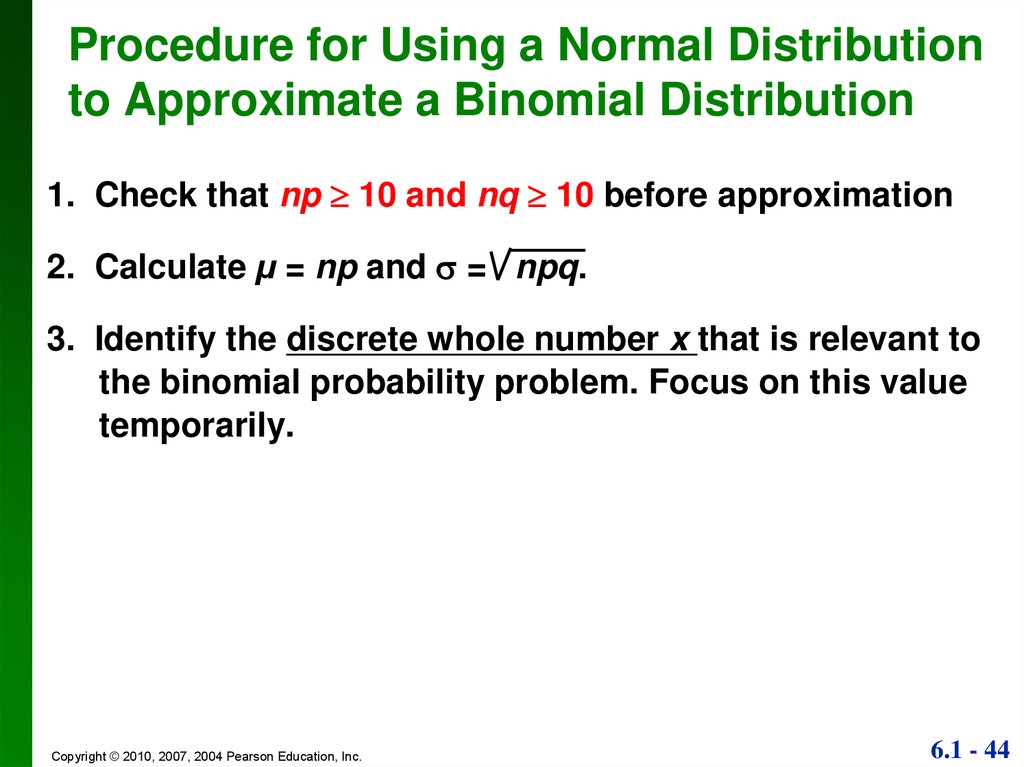
Procedure for Using a Normal Distribution
to Approximate a Binomial Distribution
1. Check that np 10 and nq 10 before approximation
2. Calculate µ = np and = npq.
3. Identify the discrete whole number x that is relevant to
the binomial probability problem. Focus on this value
temporarily.
Copyright © 2010, 2007, 2004 Pearson Education, Inc.
6.1 - 44

45.

Procedure for Using a Normal Distribution
to Approximate a Binomial Distribution
4. Draw a normal distribution centered about , then draw
a vertical strip area centered over x. Mark the left side
of the strip with the number equal to x – 0.5, and mark
the right side with the number equal to x + 0.5.
Consider the entire area of the entire strip to represent
the probability of the discrete whole number itself.
5. Determine whether the value of x itself is included in
the probability. Determine whether you want the
probability of at least x, at most x, more than x, fewer
than x, or exactly x. Shade the area to the right or left
of the strip; also shade the interior of the strip if and
only if x itself is to be included. This total shaded
region corresponds to the probability being sought.
Copyright © 2010, 2007, 2004 Pearson Education, Inc.
6.1 - 45

46.

Example 1
Suppose there are 213 passengers in a train and
the probability that a passenger is male is 0.5.
Find the probability that there are “at least 122
men among 213 passengers by using binomial
distribution
Copyright © 2010, 2007, 2004 Pearson Education, Inc.
6.1 - 46

47.

Example 1
Suppose there are 213 passengers in a train and
the probability that a passenger is male is 0.5.
Find the probability that there are “at least 122
men among 213 passengers by using normal
approximation
np 213 * 0.5 106.5
npq 213 * 0.5 * 0.5 7.2973
P(X 122) P(Y 121
? .5)
121.5 106.5
P( Z
) P( Z 2.06)
7.2973
Copyright © 2010, 2007, 2004 Pearson Education, Inc.
6.1 - 47

48.

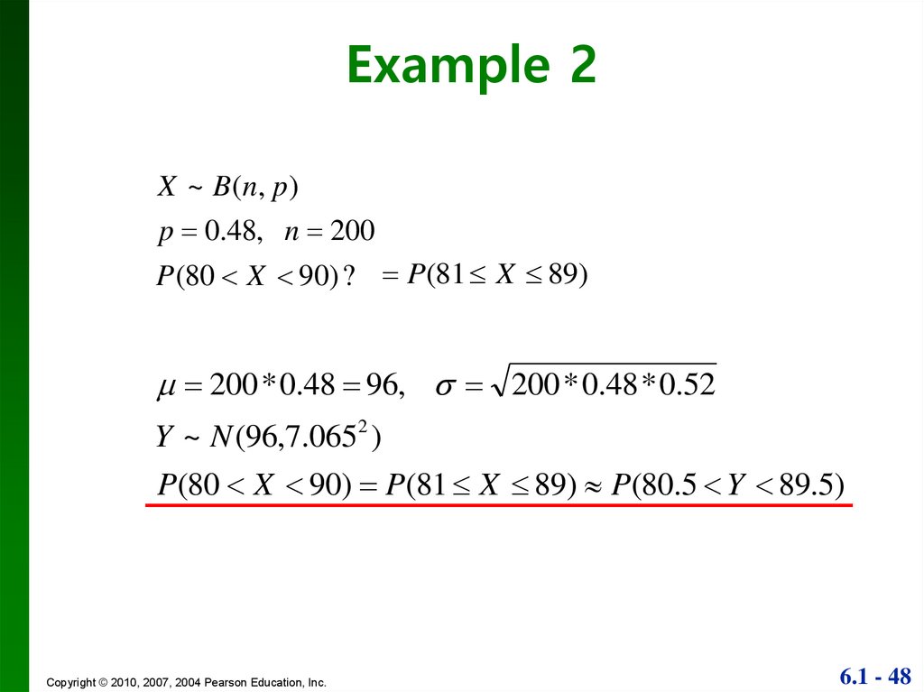
Example 2
X ~ B ( n, p )
p 0.48, n 200
P (80 X 90) ? P(81 X 89)
200 * 0.48 96, 200 * 0.48 * 0.52
Y ~ N (96,7.0652 )
P(80 X 90) P(81 X 89) P(80.5 Y 89.5)
Copyright © 2010, 2007, 2004 Pearson Education, Inc.
6.1 - 48

English Русский Rules