


 mathematics
Similar presentations:
")


")

")


Probabilistic Models. Chapter 11
1.
Probabilistic ModelsChapter 11
Copyright © 2013 Pearson Education
11-1
2.
Chapter Topics■
Types of Probability
■
Fundamentals of Probability
■
Statistical Independence and
Dependence
■
Expected Value
■
The Normal Distribution
Copyright © 2013 Pearson Education
11-2
3.
Overview■
Deterministic techniques assume that no
uncertainty exists in model parameters. Chapters 210 introduced topics that are not subject to
uncertainty or variation.
■
Probabilistic techniques include uncertainty and
assume that there can be more than one model
solution.
There is some doubt about which outcome will
occur.
Solutions may be in the form of averages.
Copyright © 2013 Pearson Education
11-3
4.
Types of ProbabilityObjective Probability
■
Classical, or a priori (prior to the occurrence),
probability is an objective probability that can be
stated prior to the occurrence of the event. It is
based on the logic of the process producing the
outcomes.
■
Objective probabilities that are stated after the
outcomes of an event have been observed are
relative frequencies, based on observation of past
occurrences.
■
Relative frequency is the more widely used
definition of objective probability.
Copyright © 2013 Pearson Education
11-4
5.
Types of ProbabilitySubjective Probability
Subjective probability is an estimate based on
personal belief, experience, or knowledge of a
situation.
It is often the only means available for making
probabilistic estimates.
Frequently used in making business decisions.
Different people often arrive at different subjective
probabilities.
Objective probabilities are used in this text unless
otherwise indicated.
Copyright © 2013 Pearson Education
11-5
6.
Fundamentals of ProbabilityOutcomes and Events
An experiment is an activity that results in one of
several possible outcomes which are termed
events.
The probability of an event is always greater than
or equal to zero and less than or equal to one.
The probabilities of all the events included in an
experiment must sum to one.
The events in an experiment are mutually
exclusive if only one can occur at a time.
The probabilities of mutually exclusive events
sum to one.
Copyright © 2013 Pearson Education
11-6
7.
Fundamentals of ProbabilityDistributions
■
A frequency distribution is an organization of
numerical data about the events in an experiment.
■
A list of corresponding probabilities for each
event is referred to as a probability distribution.
■
A set of events is collectively exhaustive when it
includes all the events that can occur in an
experiment.
Copyright © 2013 Pearson Education
11-7
8.
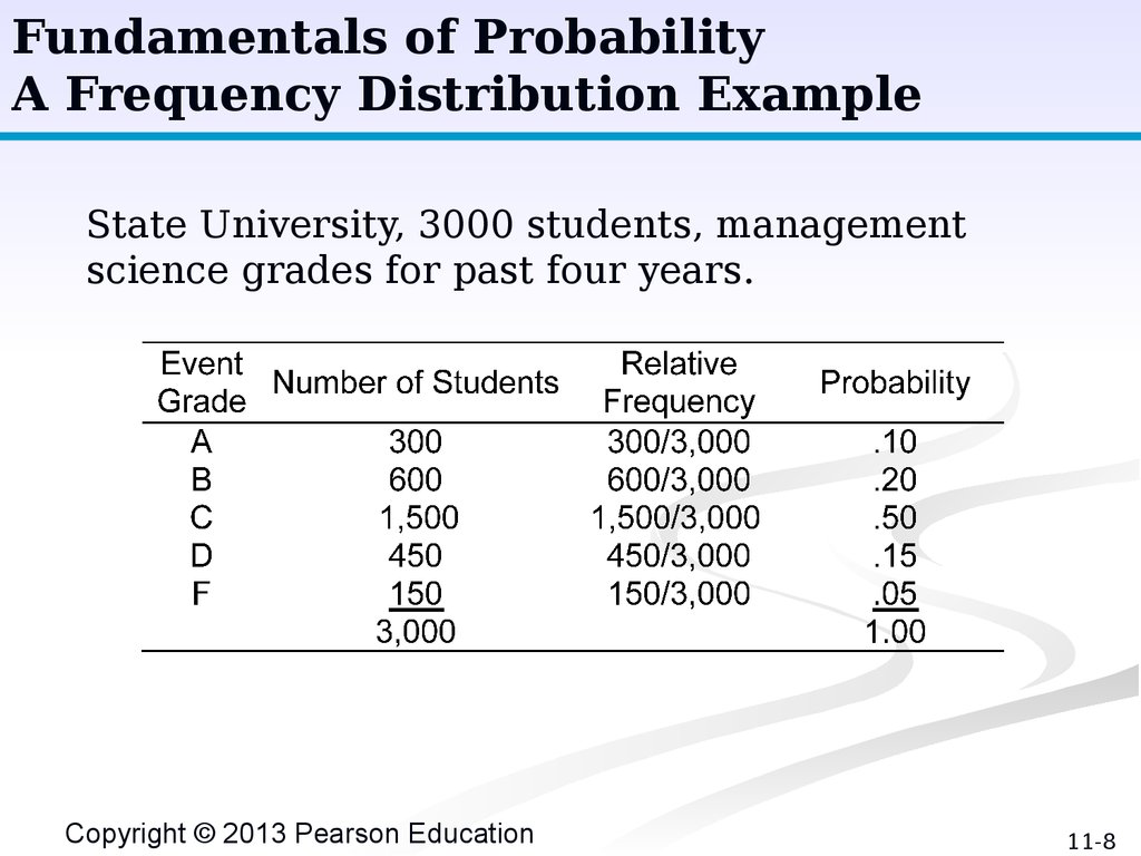
Fundamentals of ProbabilityA Frequency Distribution Example
State University, 3000 students, management
science grades for past four years.
Copyright © 2013 Pearson Education
11-8
9.
Fundamentals of ProbabilityMutually Exclusive Events & Marginal Probability
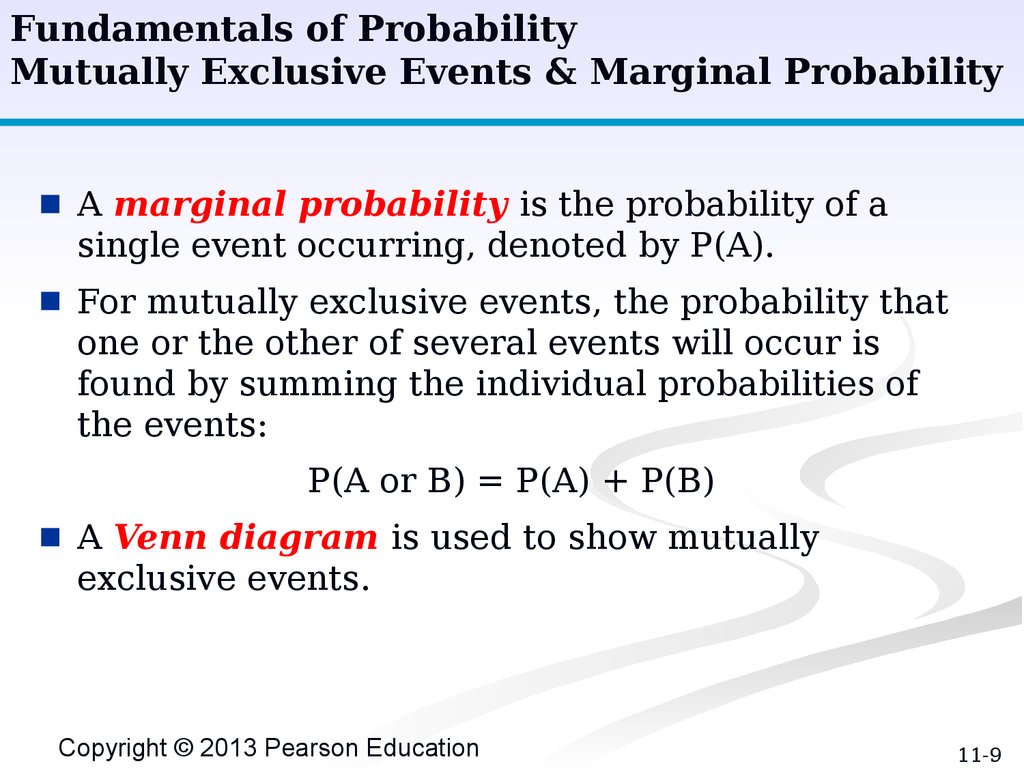
■
A marginal probability is the probability of a
single event occurring, denoted by P(A).
■
For mutually exclusive events, the probability that
one or the other of several events will occur is
found by summing the individual probabilities of
the events:
P(A or B) = P(A) + P(B)
■
A Venn diagram is used to show mutually
exclusive events.
Copyright © 2013 Pearson Education
11-9
10.
Fundamentals of ProbabilityMutually Exclusive Events & Marginal Probability
Figure 11.1
Venn Diagram for Mutually
Exclusive Events
Copyright © 2013 Pearson Education
11-
11.
Fundamentals of ProbabilityNon-Mutually Exclusive Events & Joint Probability
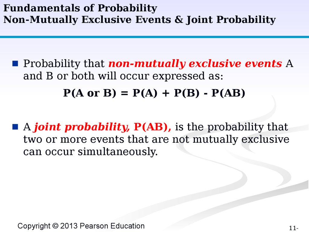
■
Probability that non-mutually exclusive events A
and B or both will occur expressed as:
P(A or B) = P(A) + P(B) - P(AB)
■
A joint probability, P(AB), is the probability that
two or more events that are not mutually exclusive
can occur simultaneously.
Copyright © 2013 Pearson Education
11-
12.
Fundamentals of ProbabilityNon-Mutually Exclusive Events & Joint Probability
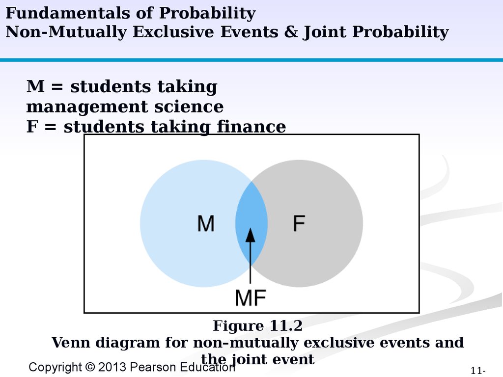
M = students taking
management science
F = students taking finance
Figure 11.2
Venn diagram for non–mutually exclusive events and
the joint event
Copyright © 2013 Pearson Education
11-
13.
Fundamentals of ProbabilityCumulative Probability Distribution
■
Can be developed by adding the probability of an event
to the sum of all previously listed probabilities in a
probability distribution.
■
Probability that a student will get a grade of C or
higher:
P(A or B or C) = P(A) + P(B) + P(C) = .10 + .20 + .50 = .
80
Copyright © 2013 Pearson Education
11-
14.
Statistical Independence and DependenceIndependent Events
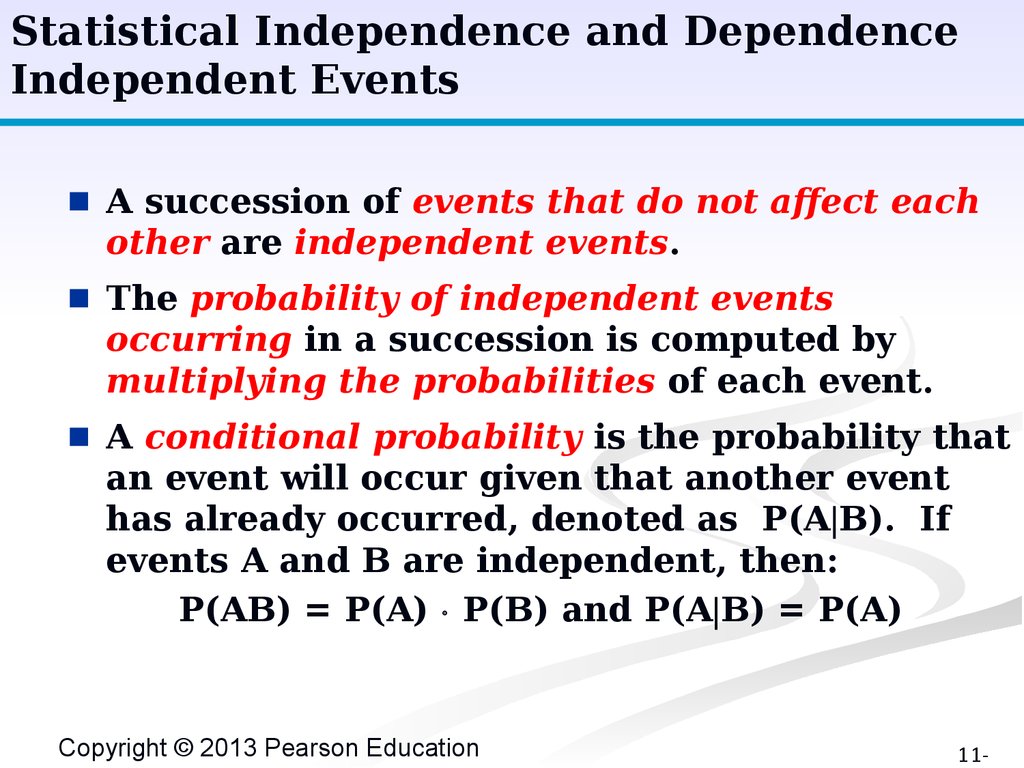
■
A succession of events that do not affect each
other are independent events.
■
The probability of independent events
occurring in a succession is computed by
multiplying the probabilities of each event.
■
A conditional probability is the probability that
an event will occur given that another event
has already occurred, denoted as P(A B). If
events A and B are independent, then:
P(AB) = P(A) P(B) and P(A B) = P(A)
Copyright © 2013 Pearson Education
11-
15.
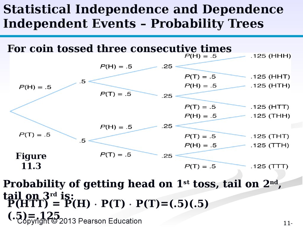
Statistical Independence and DependenceIndependent Events – Probability Trees
For coin tossed three consecutive times
Figure
11.3
Probability of getting head on 1st toss, tail on 2nd,
tail on 3rd is:
P(HTT) = P(H) P(T) P(T)=(.5)(.5)
(.5)=.125
Copyright © 2013 Pearson Education
11-
16.
Statistical Independence and DependenceIndependent Events – Bernoulli Process Definition
Properties of a Bernoulli Process:
■
■
There are two possible outcomes for each trial.
The probability of the outcome remains
constant over time.
■
The outcomes of the trials are independent.
■
The number of trials is discrete and integer.
Copyright © 2013 Pearson Education
11-
17.
Statistical Independence and DependenceIndependent Events – Binomial Distribution
A binomial probability distribution function is
used to determine the probability of a number of
successes in n trials.
It is a discrete probability distribution since the
number of successes and trials is discrete.
P(r)
n! prqn -r
r!(n-r)!
where: p = probability of a success
q = 1- p = probability of a failure
n = number of trials
r = number of successes in n trials
Copyright © 2013 Pearson Education
11-
18.
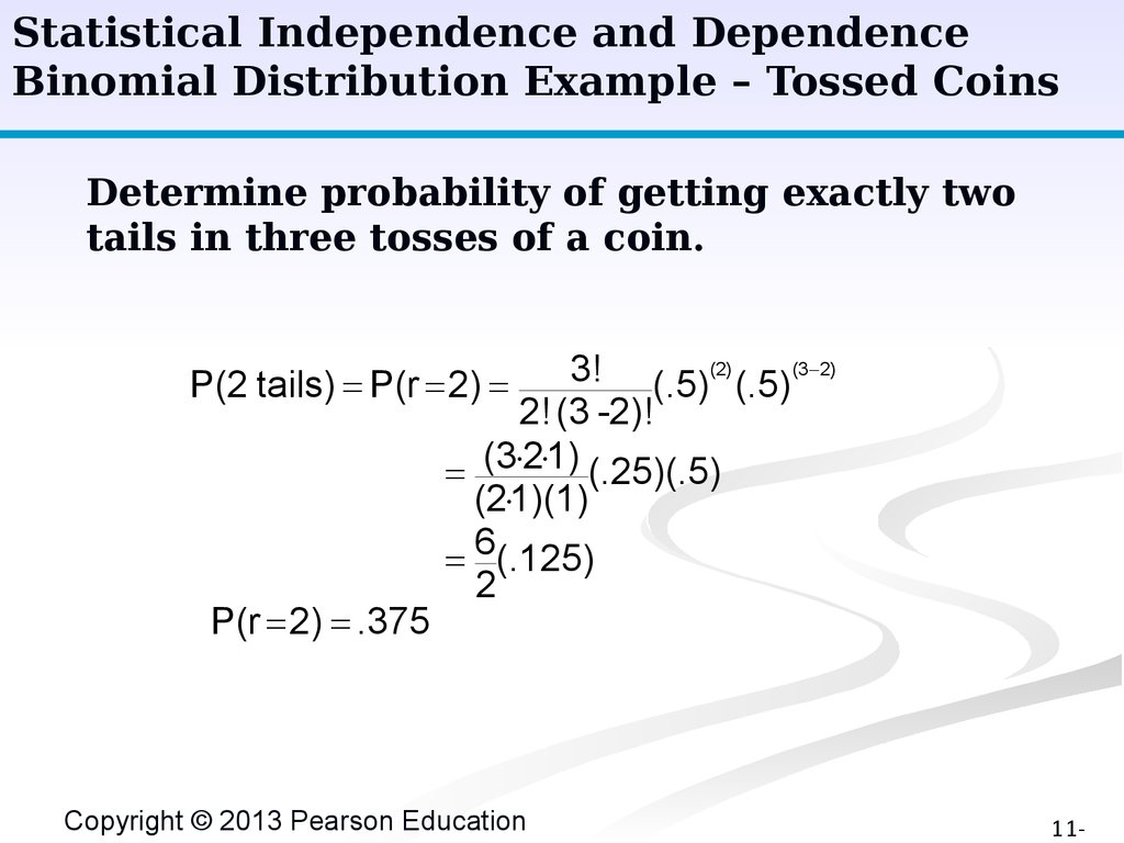
Statistical Independence and DependenceBinomial Distribution Example – Tossed Coins
Determine probability of getting exactly two
tails in three tosses of a coin.
3! (.5)(2) (.5)(3-2)
2! (3 -2)!
(.25)(.5)
(3 21)
(21)(1)
6(.125)
2
P(2 tails) P(r 2)
P(r 2) .375
Copyright © 2013 Pearson Education
11-
19.
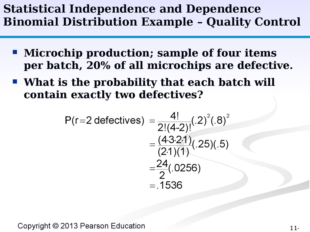
Statistical Independence and DependenceBinomial Distribution Example – Quality Control
Microchip production; sample of four items
per batch, 20% of all microchips are defective.
What is the probability that each batch will
contain exactly two defectives?
4! (.2) 2 (.8) 2
2!(4-2)!
(.25)(.5)
(4 3 21)
(21)(1)
24(.0256)
2
.1536
P(r 2 defectives)
Copyright © 2013 Pearson Education
11-
20.
Statistical Independence and DependenceBinomial Distribution Example – Quality Control
■
Four microchips tested per batch; if two or more
found defective, batch is rejected.
■
What is probability of rejecting entire batch if
batch in fact has 20% defective?
2
2
3
1
4
0
4!
4!
4!
P(r ³ 2)
(.2) (.8) +
(.2) (.8) +
(.2) (.8)
2!(4-2)!
3!(4-3)!
4!(4-4)!
.1536 + .0256 + .0016
.1808
■
Probability of less than two defectives:
P(r<2) = P(r=0) + P(r=1) = 1.0 - [P(r=2) + P(r=3) +
P(r=4)]
= 1.0 - .1808 = .8192
Copyright © 2013 Pearson Education
11-
21.
Statistical Independence and DependenceDependent Events (1 of 2)
Figure 11.4 Dependent
events
Copyright © 2013 Pearson Education
11-
22.
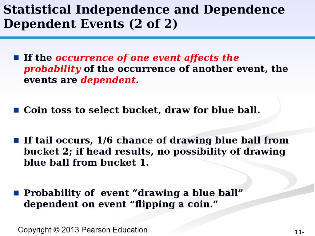
Statistical Independence and DependenceDependent Events (2 of 2)
■
If the occurrence of one event affects the
probability of the occurrence of another event, the
events are dependent.
■
Coin toss to select bucket, draw for blue ball.
■
If tail occurs, 1/6 chance of drawing blue ball from
bucket 2; if head results, no possibility of drawing
blue ball from bucket 1.
■
Probability of event “drawing a blue ball”
dependent on event “flipping a coin.”
Copyright © 2013 Pearson Education
11-
23.
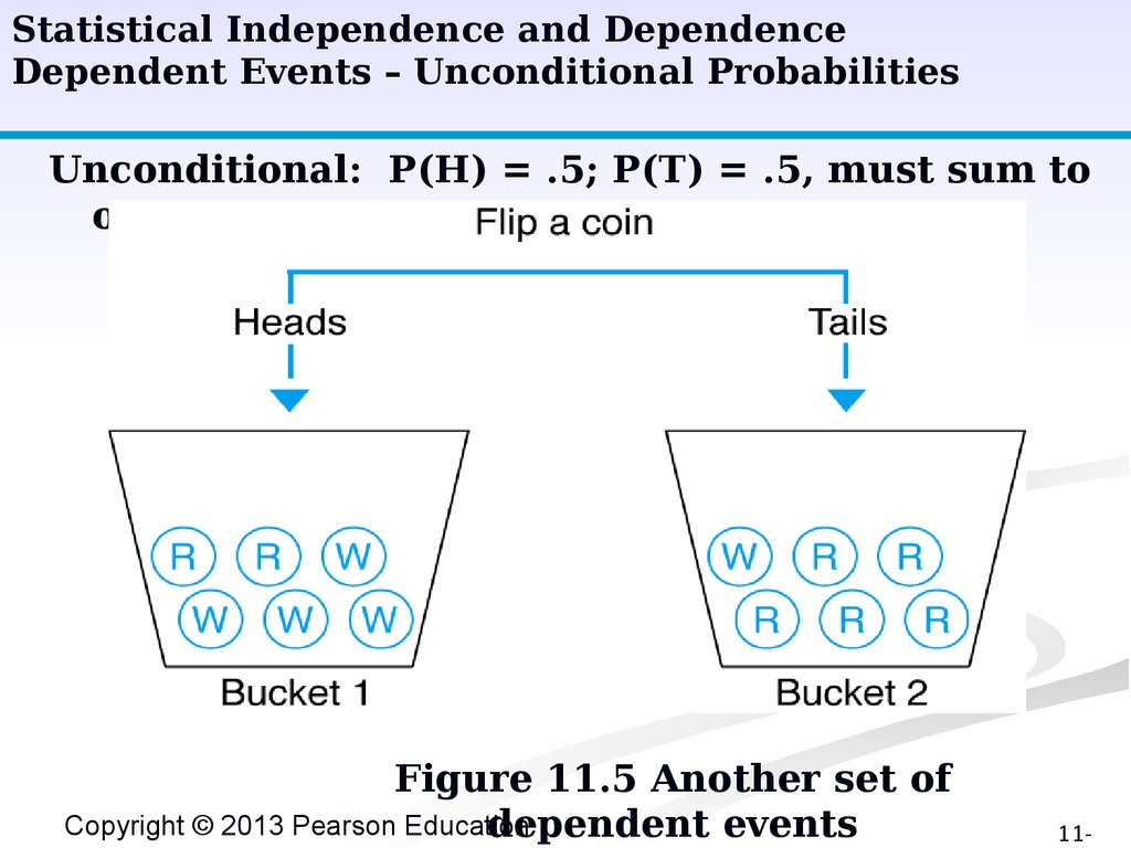
Statistical Independence and DependenceDependent Events – Unconditional Probabilities
Unconditional: P(H) = .5; P(T) = .5, must sum to
one.
Figure 11.5 Another set of
Copyright © 2013 Pearson Education
dependent events
11-
24.
Statistical Independence and DependenceDependent Events – Conditional Probabilities
Conditional: P(R H) =.33, P(W H) = .67, P(R T) = .
83, P(W T) = .17
Figure 11.6 Probability tree for
dependent
Copyright © 2013 Pearson
Education events
11-
25.
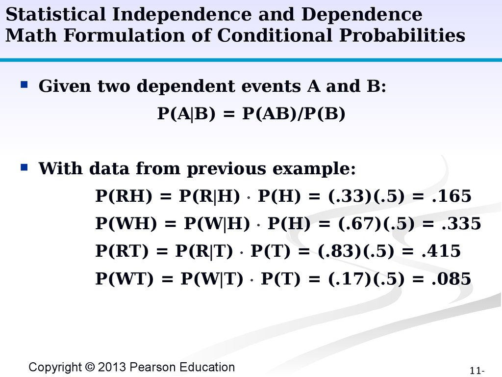
Statistical Independence and DependenceMath Formulation of Conditional Probabilities
Given two dependent events A and B:
P(A B) = P(AB)/P(B)
With data from previous example:
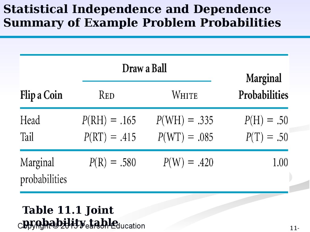
P(RH) = P(R H) P(H) = (.33)(.5) = .165
P(WH) = P(W H) P(H) = (.67)(.5) = .335
P(RT) = P(R T) P(T) = (.83)(.5) = .415
P(WT) = P(W T) P(T) = (.17)(.5) = .085
Copyright © 2013 Pearson Education
11-
26.
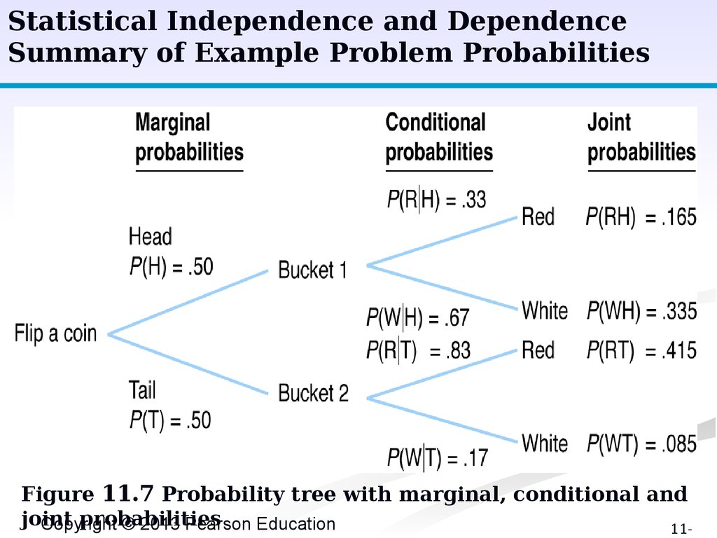
Statistical Independence and DependenceSummary of Example Problem Probabilities
Figure 11.7 Probability tree with marginal, conditional and
joint
probabilities
Copyright
© 2013 Pearson Education
11-
27.
Statistical Independence and DependenceSummary of Example Problem Probabilities
Table 11.1 Joint
probability
table
Copyright
© 2013 Pearson
Education
11-
28.
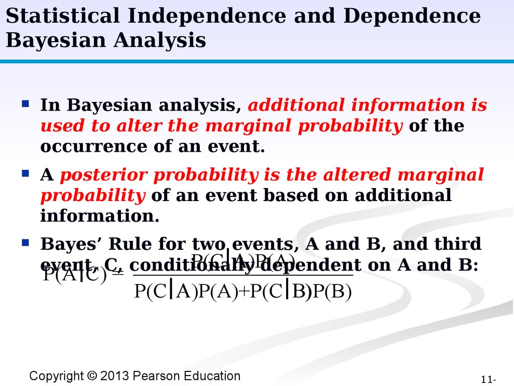
Statistical Independence and DependenceBayesian Analysis
In Bayesian analysis, additional information is
used to alter the marginal probability of the
occurrence of an event.
A posterior probability is the altered marginal
probability of an event based on additional
information.
Bayes’ Rule for two events, A and B, and third
P(CôA)P(A)
event, C, conditionally
dependent on A and B:
P(AôC) =
P(CôA)P(A)+P(CôB)P(B)
Copyright © 2013 Pearson Education
11-
29.
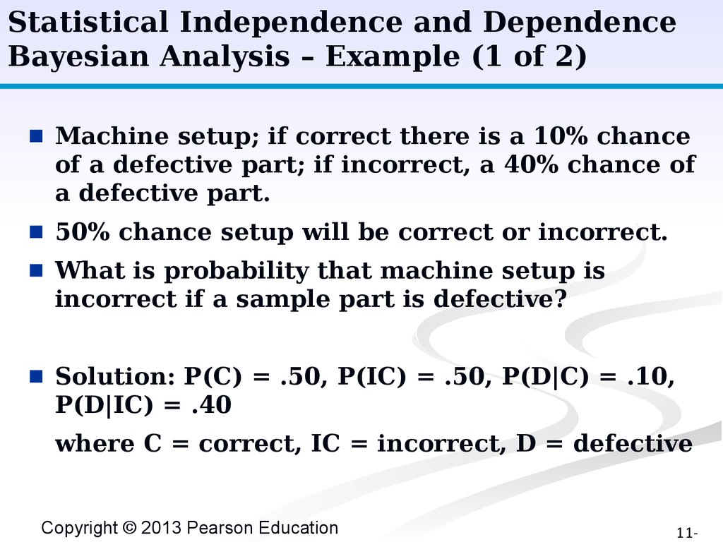
Statistical Independence and DependenceBayesian Analysis – Example (1 of 2)
■
Machine setup; if correct there is a 10% chance
of a defective part; if incorrect, a 40% chance of
a defective part.
■
50% chance setup will be correct or incorrect.
■
What is probability that machine setup is
incorrect if a sample part is defective?
■
Solution: P(C) = .50, P(IC) = .50, P(D|C) = .10,
P(D|IC) = .40
where C = correct, IC = incorrect, D = defective
Copyright © 2013 Pearson Education
11-
30.
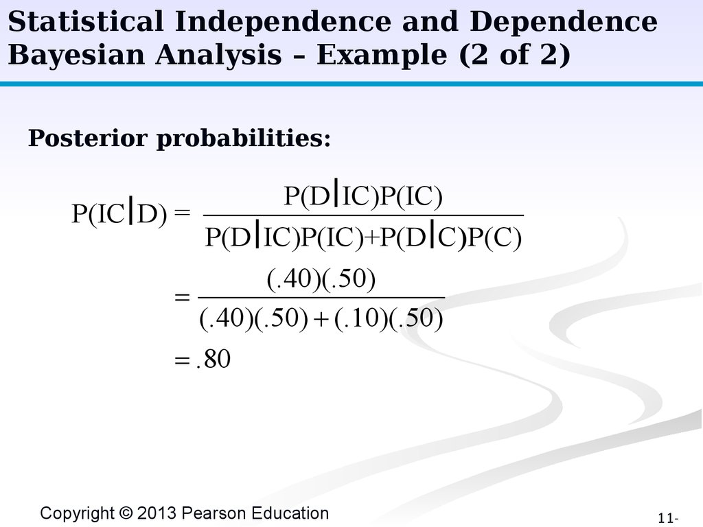
Statistical Independence and DependenceBayesian Analysis – Example (2 of 2)
Posterior probabilities:
P(DôIC)P(IC)
P(ICôD) =
P(DôIC)P(IC)+P(DôC )P(C)
(.40)(.50)
(.40)(.50) + (.10)(.50)
.80
Copyright © 2013 Pearson Education
11-
31.
Expected ValueRandom Variables
■
When the values of variables occur in no
particular order or sequence, the variables are
referred to as random variables.
■
Random variables are represented symbolically
by a letter x, y, z, etc.
■
Although exact values of random variables are
not known prior to events, it is possible to
assign a probability to the occurrence of
possible values.
Copyright © 2013 Pearson Education
11-
32.
Expected ValueExample (1 of 4)
■
Machines break down 0, 1, 2, 3, or 4 times per
month.
■
Relative frequency of breakdowns , or a
probability distribution:
Copyright © 2013 Pearson Education
11-
33.
Expected ValueExample (2 of 4)
■
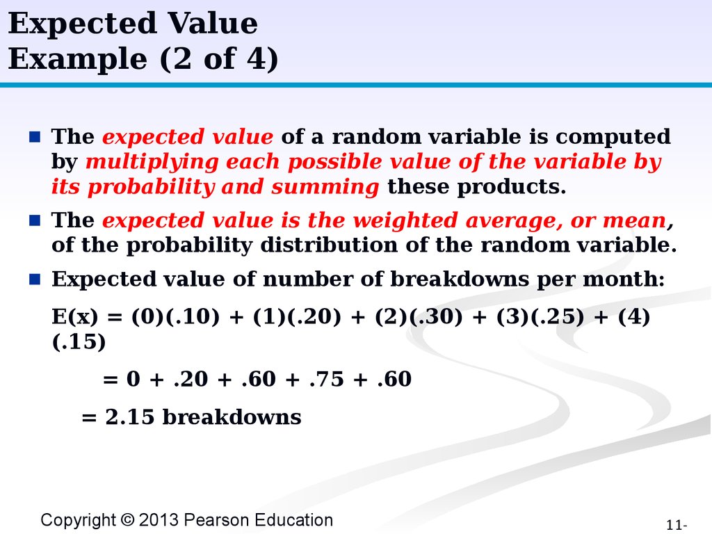
The expected value of a random variable is computed
by multiplying each possible value of the variable by
its probability and summing these products.
■
The expected value is the weighted average, or mean,
of the probability distribution of the random variable.
■
Expected value of number of breakdowns per month:
E(x) = (0)(.10) + (1)(.20) + (2)(.30) + (3)(.25) + (4)
(.15)
= 0 + .20 + .60 + .75 + .60
= 2.15 breakdowns
Copyright © 2013 Pearson Education
11-
34.
Expected ValueExample (3 of 4)
■
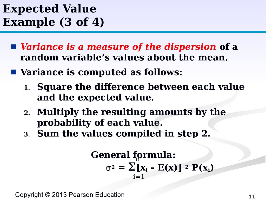
Variance is a measure of the dispersion of a
random variable’s values about the mean.
■
Variance is computed as follows:
1.
Square the difference between each value
and the expected value.
2.
Multiply the resulting amounts by the
probability of each value.
Sum the values compiled in step 2.
3.
General formula:
n
2 = [xi - E(x)]
i=1
Copyright © 2013 Pearson Education
2
P(xi)
11-
35.
Expected ValueExample (4 of 4)
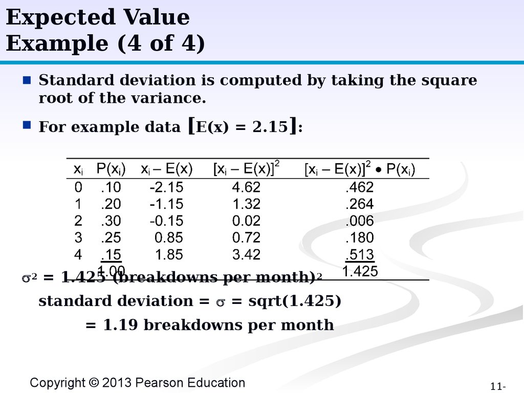
■
Standard deviation is computed by taking the square
root of the variance.
■
For example data
[E(x) = 2.15]:
2 = 1.425 (breakdowns per month)2
standard deviation = = sqrt(1.425)
= 1.19 breakdowns per month
Copyright © 2013 Pearson Education
11-
36.
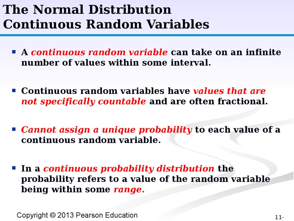
The Normal DistributionContinuous Random Variables
A continuous random variable can take on an infinite
number of values within some interval.
Continuous random variables have values that are
not specifically countable and are often fractional.
Cannot assign a unique probability to each value of a
continuous random variable.
In a continuous probability distribution the
probability refers to a value of the random variable
being within some range.
Copyright © 2013 Pearson Education
11-
37.
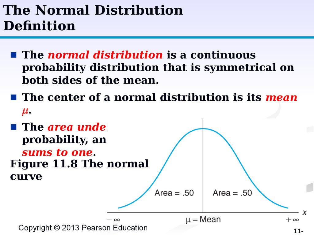
The Normal DistributionDefinition
■
The normal distribution is a continuous
probability distribution that is symmetrical on
both sides of the mean.
■
The center of a normal distribution is its mean
.
The area under the normal curve represents
probability, and the total area under the curve
sums to one.
Figure 11.8 The normal
curve
■
Copyright © 2013 Pearson Education
11-
38.
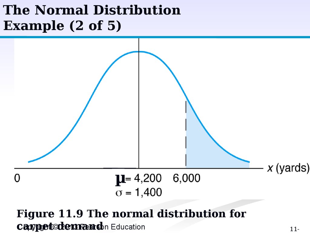
The Normal DistributionExample (1 of 5)
■
Mean weekly carpet sales of 4,200 yards, with
a standard deviation of 1,400 yards.
■
What is the probability of sales exceeding
6,000 yards?
■
= 4,200 yd; = 1,400 yd; probability that
number of yards of carpet will be equal to or
greater than 6,000 expressed as: P(x³6,000).
Copyright © 2013 Pearson Education
11-
39.
The Normal DistributionExample (2 of 5)
P(x≥6,000)
-
µ
Figure 11.9 The normal distribution for
Copyright ©demand
2013 Pearson Education
carpet
11-
40.
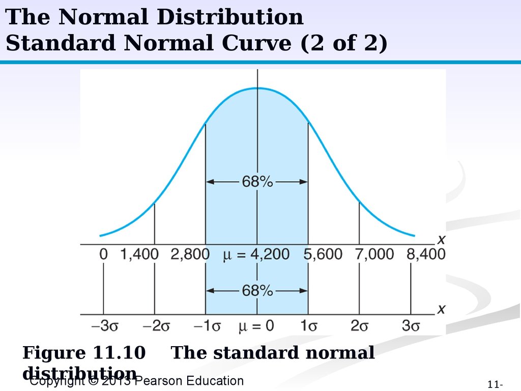
The Normal DistributionStandard Normal Curve (1 of 2)
■
The area or probability under a normal curve
is measured by determining the number of
standard deviations the value of a random
variable x is from the mean.
■
Number of standard deviations a value is from
the mean designated
X -as
Z.
Z
Copyright © 2013 Pearson Education
11-
41.
The Normal DistributionStandard Normal Curve (2 of 2)
Figure 11.10 The standard normal
distribution
Copyright © 2013 Pearson Education
11-
42.
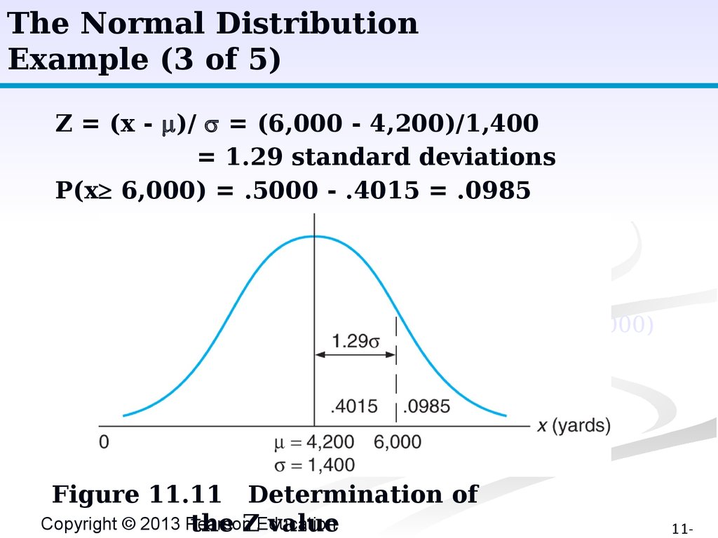
The Normal DistributionExample (3 of 5)
Z = (x - )/ = (6,000 - 4,200)/1,400
= 1.29 standard deviations
P(x³ 6,000) = .5000 - .4015 = .0985
P(x≥6,000)
Figure 11.11 Determination of
Copyright © 2013 Pearson
the ZEducation
value
11-
43.
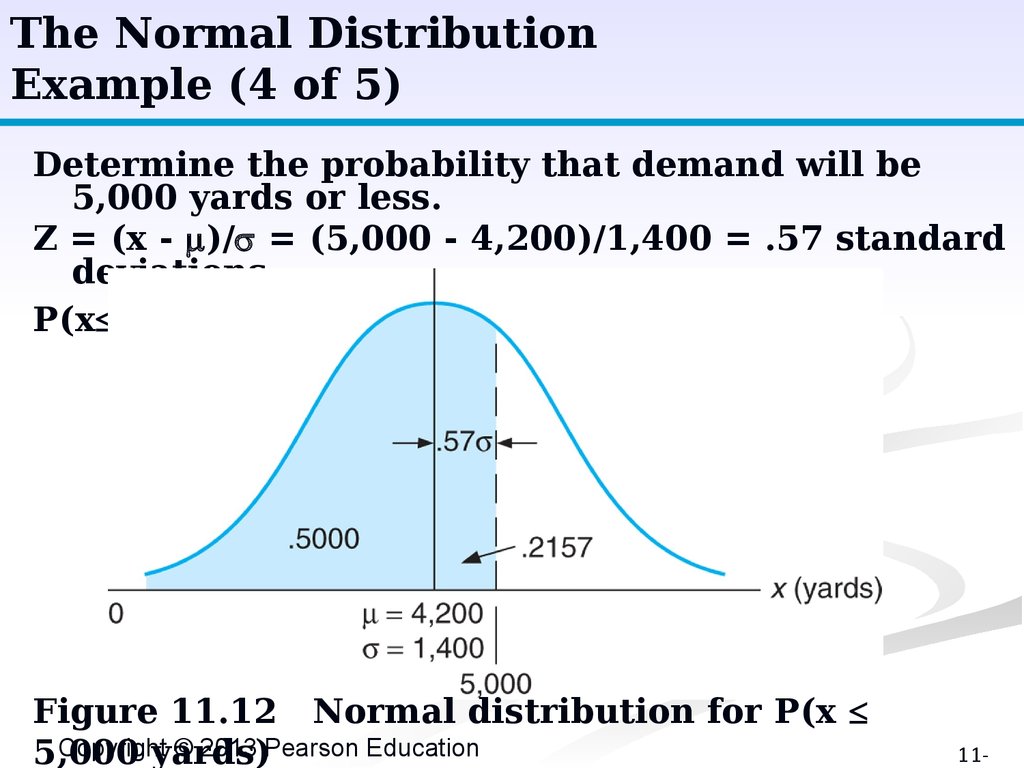
The Normal DistributionExample (4 of 5)
Determine the probability that demand will be
5,000 yards or less.
Z = (x - )/ = (5,000 - 4,200)/1,400 = .57 standard
deviations
P(x 5,000) = .5000 + .2157 = .7157
Figure 11.12 Normal distribution for P(x
Copyright
© 2013 Pearson Education
5,000
yards)
11-
44.
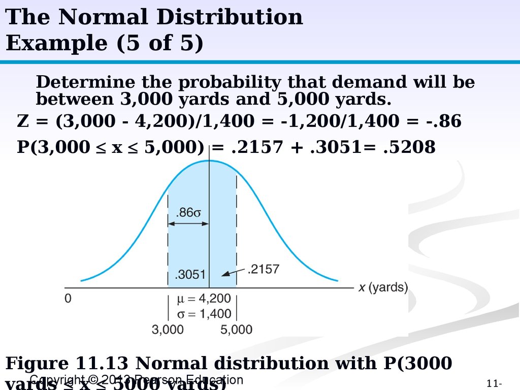
The Normal DistributionExample (5 of 5)
Determine the probability that demand will be
between 3,000 yards and 5,000 yards.
Z = (3,000 - 4,200)/1,400 = -1,200/1,400 = -.86
P(3,000 x 5,000) = .2157 + .3051= .5208
Figure 11.13 Normal distribution with P(3000
Copyright
Pearson
Education
yards
x© 2013
5000
yards)
11-
45.
The Normal DistributionSample Mean and Variance
■
The population mean and variance are for the
entire set of data being analyzed.
■
The sample mean and variance are derived
from a subset of the population data and are
used to make inferences about the population.
Copyright © 2013 Pearson Education
11-
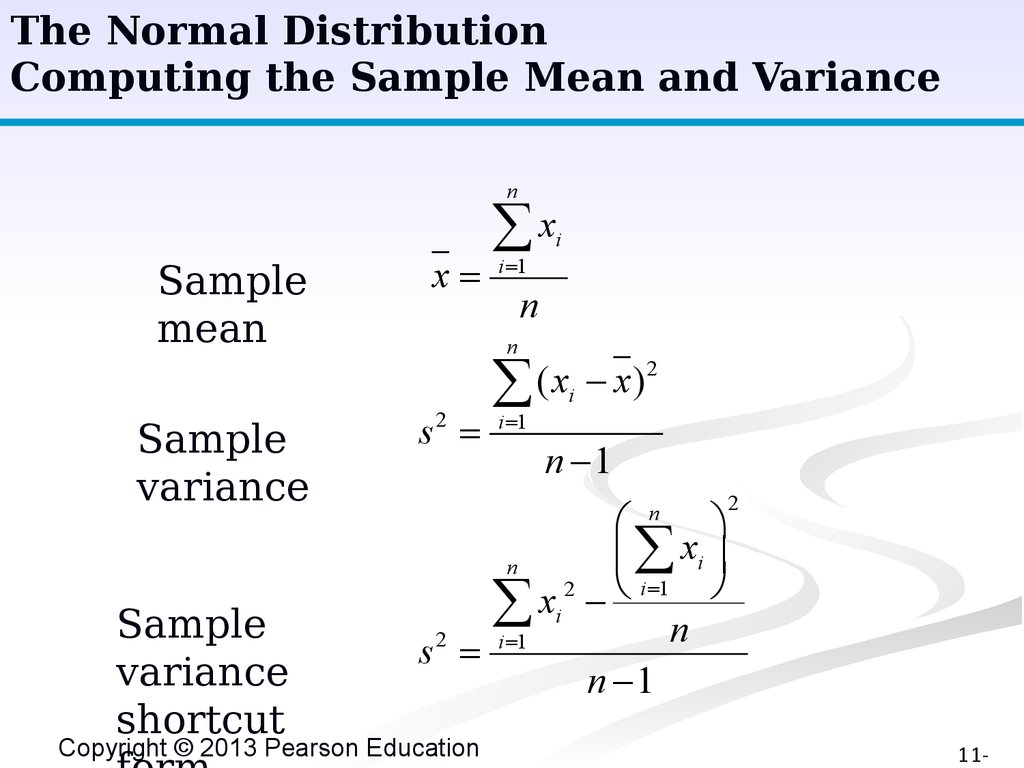
46.
The Normal DistributionComputing the Sample Mean and Variance
n
Sample
mean
x
Sample
variance
s2
Sample
variance
shortcut
åx
i 1
i
n
n
2
(
x
x
)
å i
i 1
n -1
æ
ö
ç å xi ÷
n
2
è i 1 ø
x
å
i
n
2
i 1
s
n -1
Copyright © 2013 Pearson Education
n
2
11-
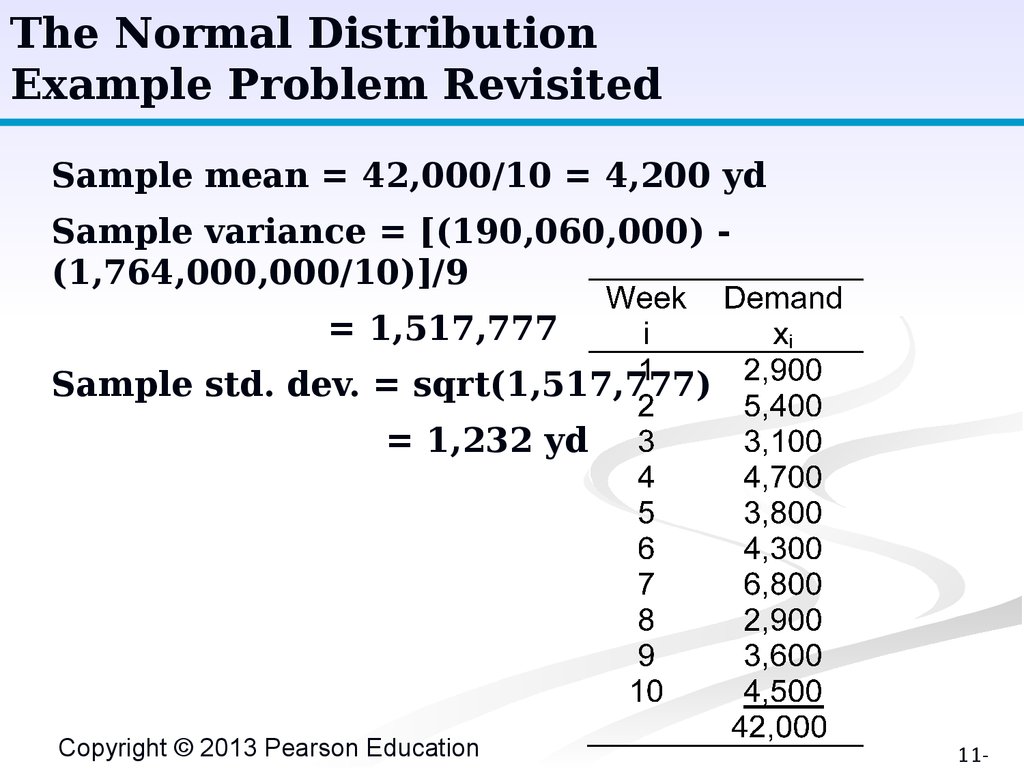
47.
The Normal DistributionExample Problem Revisited
Sample mean = 42,000/10 = 4,200 yd
Sample variance = [(190,060,000) (1,764,000,000/10)]/9
= 1,517,777
Sample std. dev. = sqrt(1,517,777)
= 1,232 yd
Copyright © 2013 Pearson Education
11-
48.
The Normal DistributionChi-Square Test for Normality (1 of 2)
■
It can never be simply assumed that data are
normally distributed.
■
The chi-square test is used to determine if a
set of data fit a particular distribution.
■
The chi-square test compares an observed
frequency distribution with a theoretical
frequency distribution (testing the goodnessof-fit).
Copyright © 2013 Pearson Education
11-
49.
The Normal DistributionChi-Square Test for Normality (2 of 2)
■
In the test, the actual number of frequencies in
each range of frequency distribution is compared to
the theoretical frequencies that should occur in
each range if the data follow a particular
distribution.
■
A chi-square statistic is then calculated and
compared to a number, called a critical value, from
a chi-square table.
■
If the test statistic is greater than the critical value,
the distribution does not follow the distribution
being tested; if it is less, the distribution fits.
■
The chi-square test is a form of hypothesis testing.
Copyright © 2013 Pearson Education
11-
50.
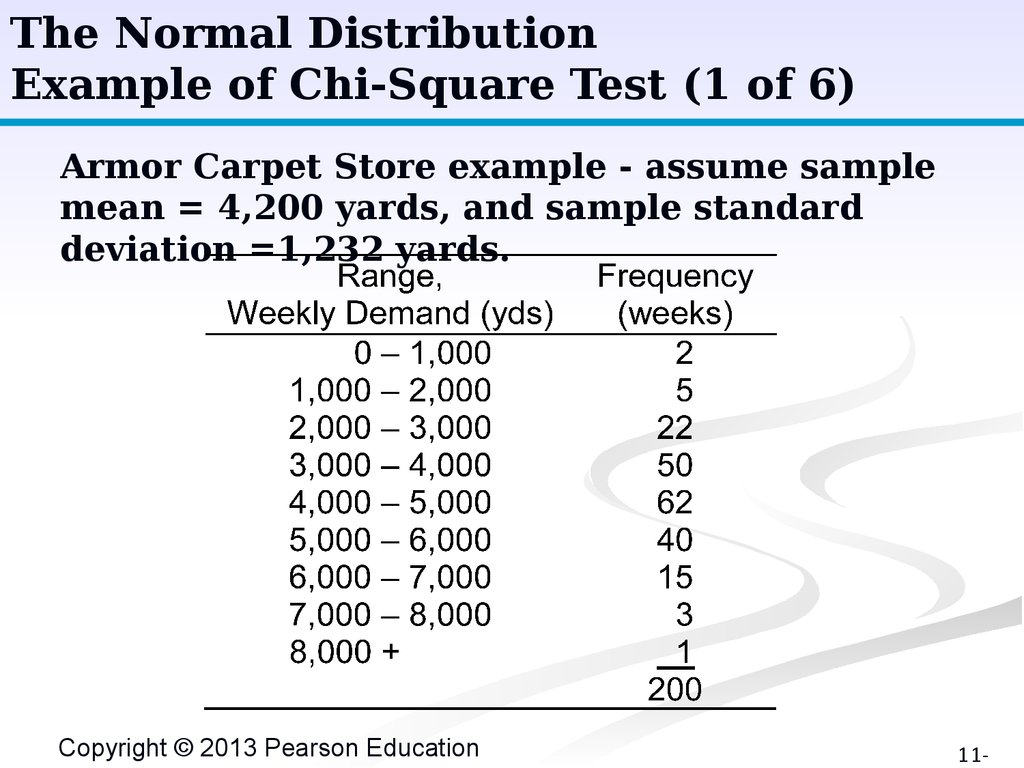
The Normal DistributionExample of Chi-Square Test (1 of 6)
Armor Carpet Store example - assume sample
mean = 4,200 yards, and sample standard
deviation =1,232 yards.
Copyright © 2013 Pearson Education
11-
51.
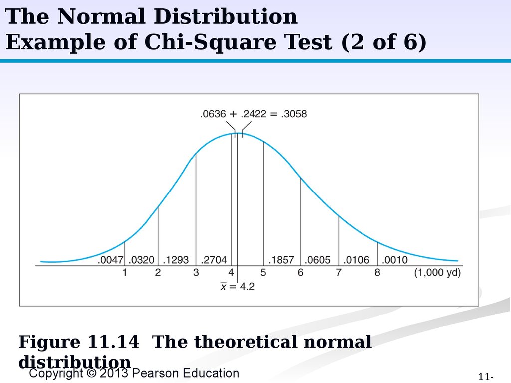
The Normal DistributionExample of Chi-Square Test (2 of 6)
Figure 11.14 The theoretical normal
distribution
Copyright © 2013 Pearson Education
11-
52.
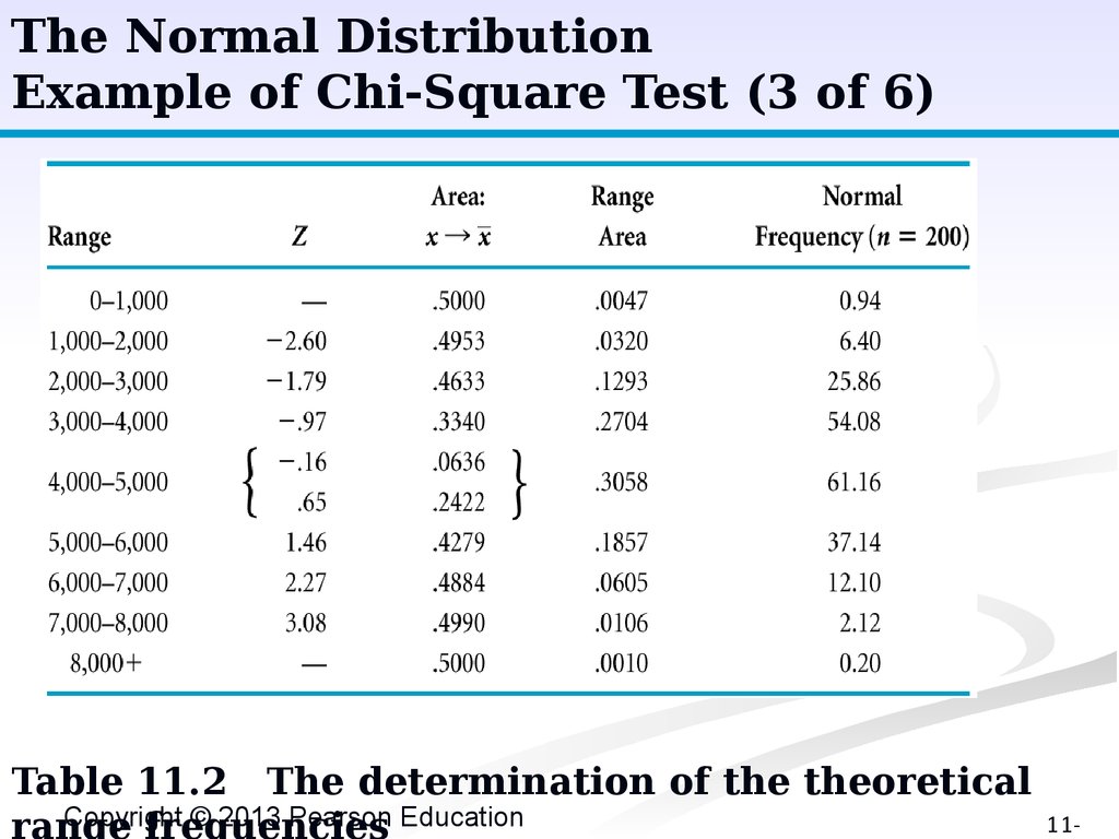
The Normal DistributionExample of Chi-Square Test (3 of 6)
Table 11.2
The determination of the theoretical
Copyright © 2013 Pearson Education
11-
53.
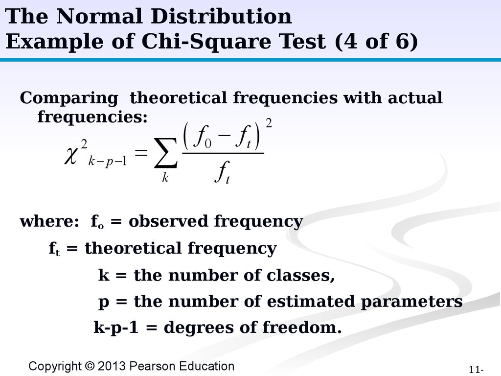
The Normal DistributionExample of Chi-Square Test (4 of 6)
Comparing theoretical frequencies with actual
frequencies:
2
c
2
k - p -1
å
k
(
f0 - ft )
ft
where: fo = observed frequency
ft = theoretical frequency
k = the number of classes,
p = the number of estimated parameters
k-p-1 = degrees of freedom.
Copyright © 2013 Pearson Education
11-
54.
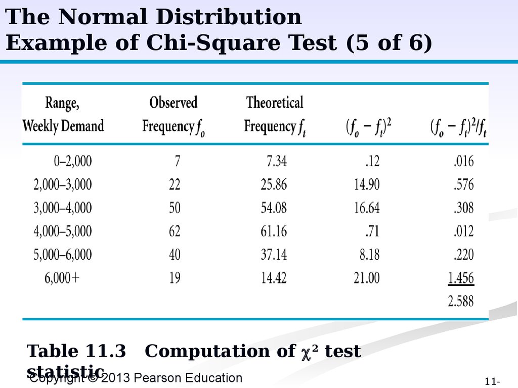
The Normal DistributionExample of Chi-Square Test (5 of 6)
Table 11.3 Computation of c 2 test
statistic
Copyright © 2013 Pearson Education
11-
55.
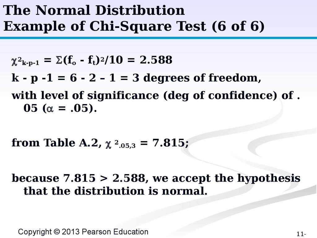
The Normal DistributionExample of Chi-Square Test (6 of 6)
c 2k-p-1 = (fo - ft)2/10 = 2.588
k - p -1 = 6 - 2 – 1 = 3 degrees of freedom,
with level of significance (deg of confidence) of .
05 ( = .05).
from Table A.2, c
2
.05,3
= 7.815;
because 7.815 > 2.588, we accept the hypothesis
that the distribution is normal.
Copyright © 2013 Pearson Education
11-
56.
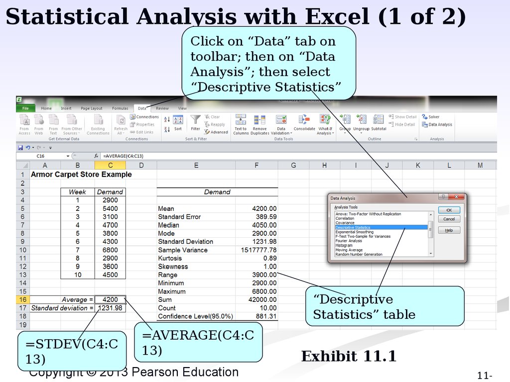
Statistical Analysis with Excel (1 of 2)Click on “Data” tab on
toolbar; then on “Data
Analysis”; then select
“Descriptive Statistics”
“Descriptive
Statistics” table
=AVERAGE(C4:C
=STDEV(C4:C
13)
13)
Copyright © 2013 Pearson Education
Exhibit 11.1
11-
57.
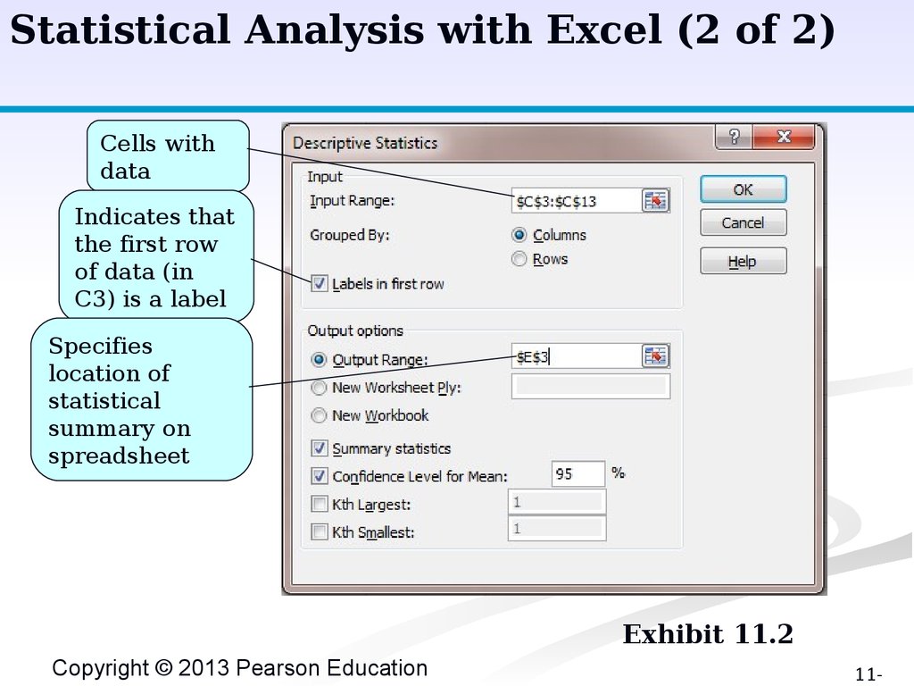
Statistical Analysis with Excel (2 of 2)Cells with
data
Indicates that
the first row
of data (in
C3) is a label
Specifies
location of
statistical
summary on
spreadsheet
Exhibit 11.2
Copyright © 2013 Pearson Education
11-
58.
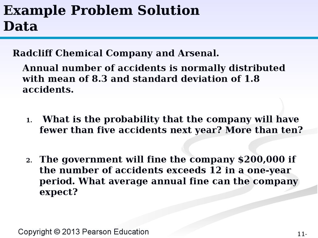
Example Problem SolutionData
Radcliff Chemical Company and Arsenal.
Annual number of accidents is normally distributed
with mean of 8.3 and standard deviation of 1.8
accidents.
1.
What is the probability that the company will have
fewer than five accidents next year? More than ten?
2.
The government will fine the company $200,000 if
the number of accidents exceeds 12 in a one-year
period. What average annual fine can the company
expect?
Copyright © 2013 Pearson Education
11-
59.
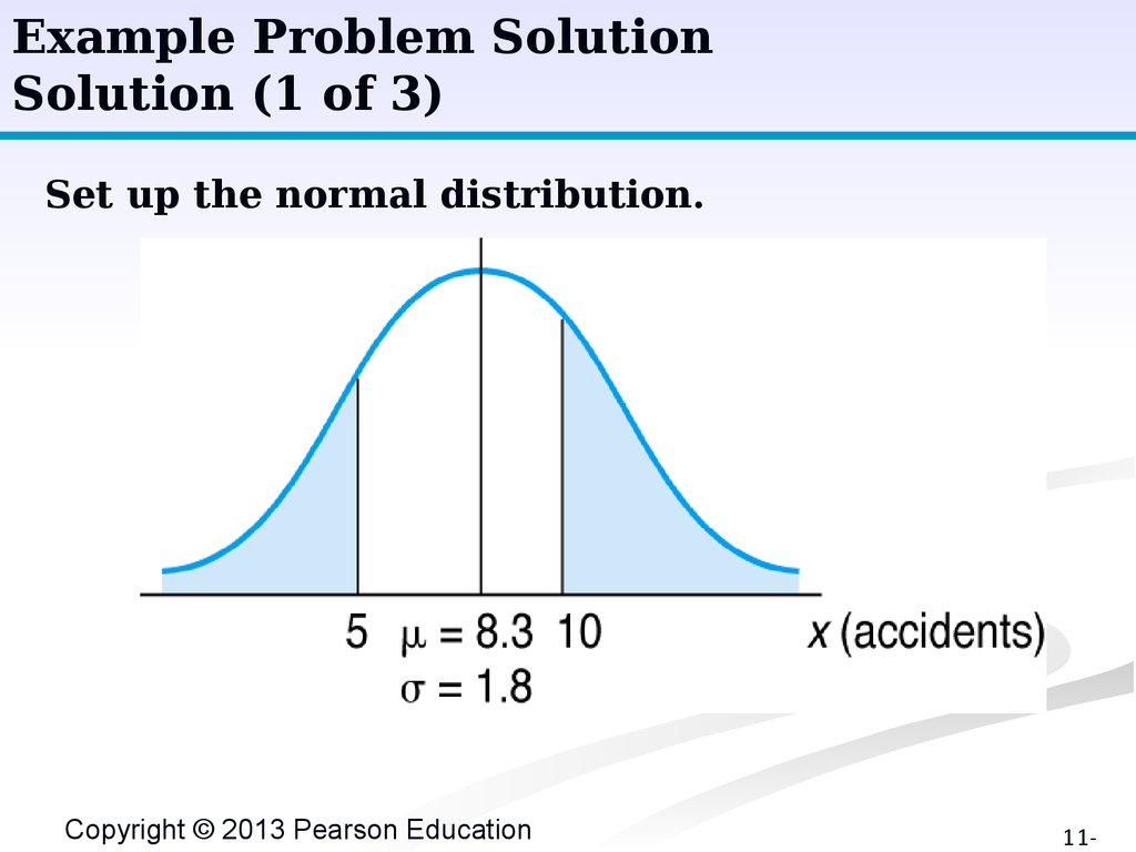
Example Problem SolutionSolution (1 of 3)
Set up the normal distribution.
Copyright © 2013 Pearson Education
11-
60.
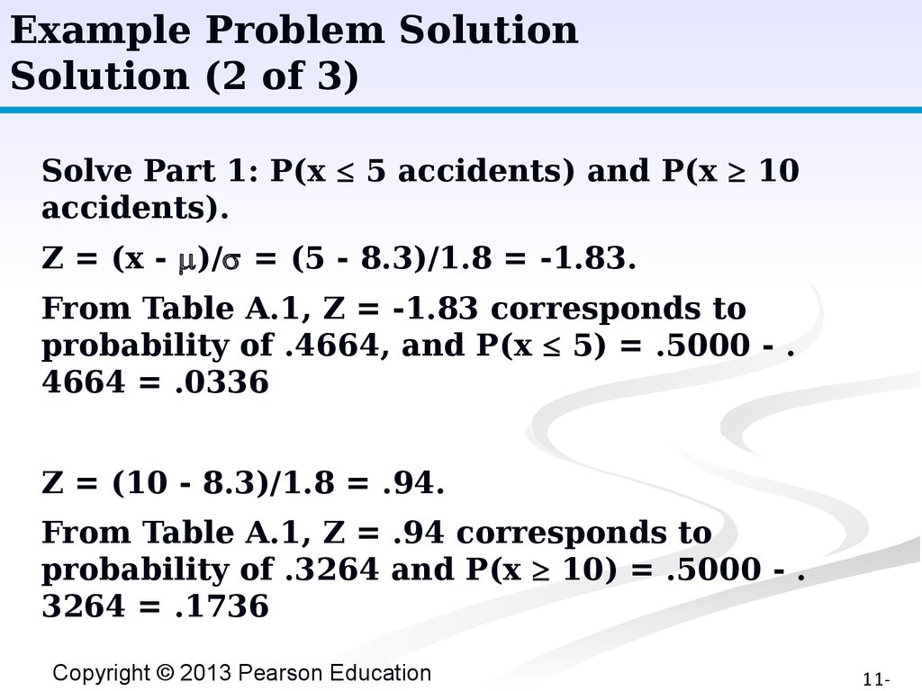
Example Problem SolutionSolution (2 of 3)
Solve Part 1: P(x 5 accidents) and P(x ³ 10
accidents).
Z = (x - )/ = (5 - 8.3)/1.8 = -1.83.
From Table A.1, Z = -1.83 corresponds to
probability of .4664, and P(x 5) = .5000 - .
4664 = .0336
Z = (10 - 8.3)/1.8 = .94.
From Table A.1, Z = .94 corresponds to
probability of .3264 and P(x ³ 10) = .5000 - .
3264 = .1736
Copyright © 2013 Pearson Education
11-
61.
Example Problem SolutionSolution (3 of 3)
Solve Part 2:
P(x ³ 12 accidents)
Z = 2.06, corresponding to probability of .4803.
P(x ³ 12) = .5000 - .4803 = .0197, expected
annual fine
= $200,000(.0197) = $3,940
Copyright © 2013 Pearson Education
11-
62.
All rights reserved. No part of this publication may be reproduced, stored in a retrievalsystem, or transmitted, in any form or by any means, electronic, mechanical, photocopying,
recording, or otherwise, without the prior written permission of the publisher.
Printed in the United States of America.
Copyright © 2013 Pearson Education
11-