Probability Random Variables Preparatory Notes

1. NATCOR STOCHASTIC MODELLING (preliminary reading) Introduction to Probability & Random Variables

NATCOR
STOCHASTIC MODELLING
(preliminary reading)
Introduction to Probability
& Random Variables
1.
2.
IMPORTANT
This material is designed to be viewed is two ways:
In ‘Slide Show’ format, to take advantage of the animations;
In ‘Notes Page’ format, so that you can see the accompanying notes.
You might find it helps to print out the latter (to refer to) whilst viewing the former.
NATCOR: Stochastic Modelling 2017 – Preliminary Reading

2. Overview

Basic Probability
• Concepts
Continuous Random Variables
• Definition
• Laws and Notation
• Probability Density Function
• Conditional Probability
• Probability as an Integral
• Total Law of Probability
• Mean and Variance
Discrete Random Variables
• Conditional Expectation
• Definition
• Probability Mass Function • Exponential Distribution
• Normal Distribution
• Mean and Variance
• Conditional Expectation
• Poisson Distribution
NATCOR: Stochastic Modelling 2017 – Preliminary Reading

3. BASIC PROBABILITY CONCEPTS: ‘Experiments’ and ‘Events’

Experiment: an action whose outcome is uncertain (roll a die)
Sample Space: set of all possible outcomes of an experiment (S = {1, 2, 3,
4, 5, 6})
Event: a subset of outcomes that is of interest to us (e.g. event 1 = even
number, event 2 = higher than 4, event 3 = throw a 2, etc)
Probability: measure of how likely an event is to occur (between 0 and 1)
NATCOR: Stochastic Modelling 2017 – Preliminary Reading

4.

How to measure probability
•Probability: measure of how likely an event is to occur (between 0 and 1)
• Classical Definition
- Calculate, assuming events equally likely
• Relative Frequency Approach
- Doing an experiment, using historical data
• Subjective/Bayesian Probability
- Trusting instinct, using judgement
NATCOR: Stochastic Modelling 2017 – Preliminary Reading

5.

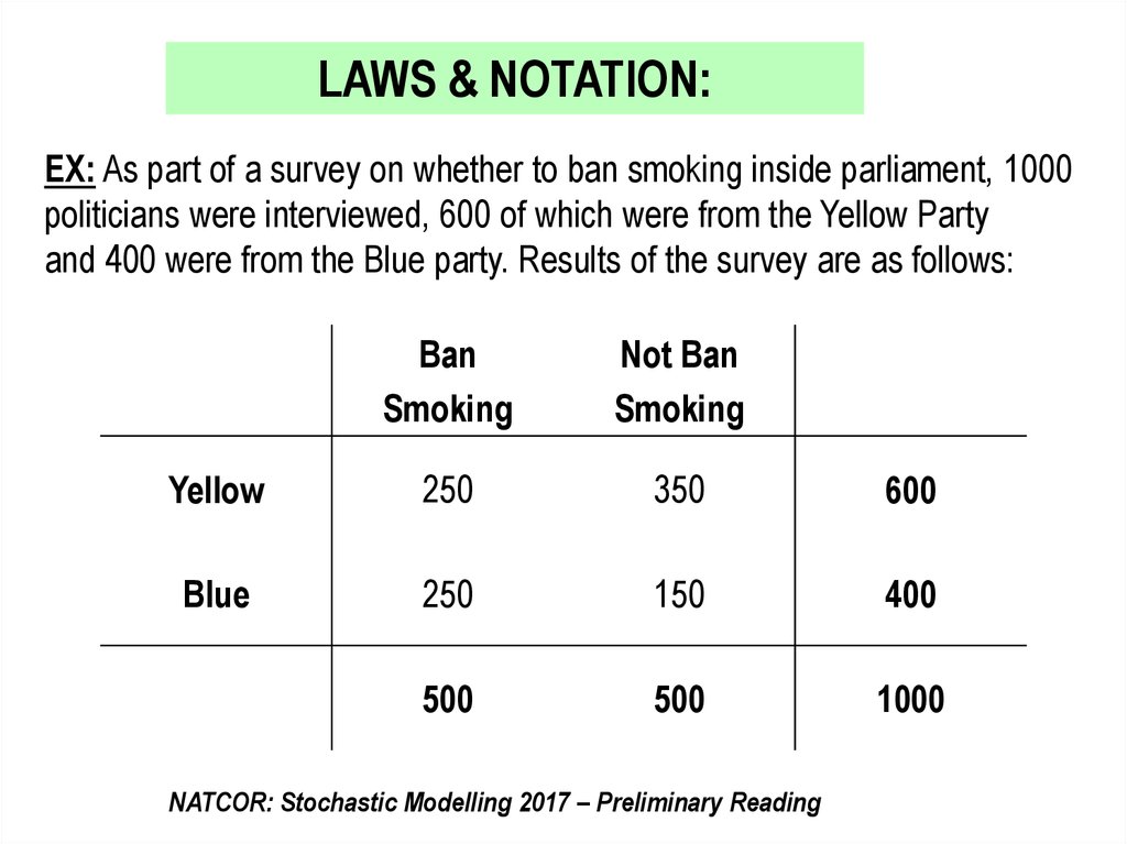
LAWS & NOTATION:
EX: As part of a survey on whether to ban smoking inside parliament, 1000
politicians were interviewed, 600 of which were from the Yellow Party
and 400 were from the Blue party. Results of the survey are as follows:
Ban
Smoking
Not Ban
Smoking
Yellow
250
350
600
Blue
250
150
400
500
500
1000
NATCOR: Stochastic Modelling 2017 – Preliminary Reading

6.

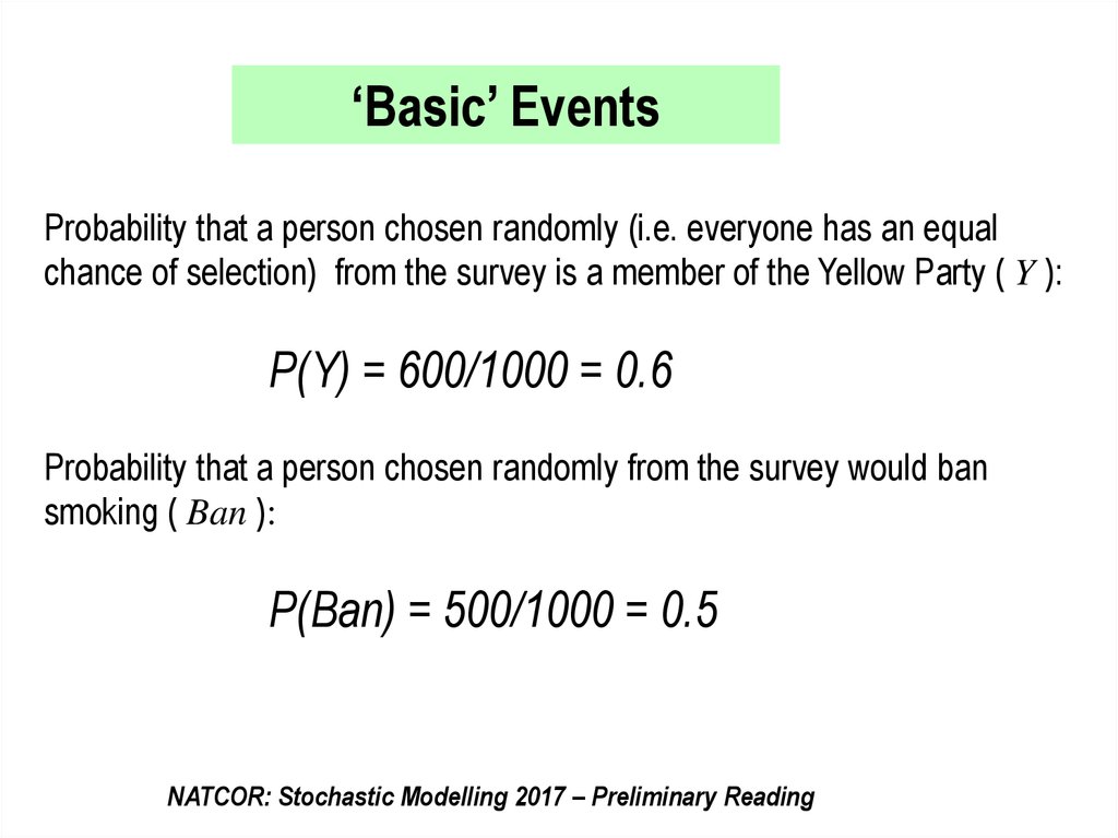
‘Basic’ Events
Probability that a person chosen randomly (i.e. everyone has an equal
chance of selection) from the survey is a member of the Yellow Party ( Y ):
P(Y) = 600/1000 = 0.6
Probability that a person chosen randomly from the survey would ban
smoking ( Ban ):
P(Ban) = 500/1000 = 0.5
NATCOR: Stochastic Modelling 2017 – Preliminary Reading

7.

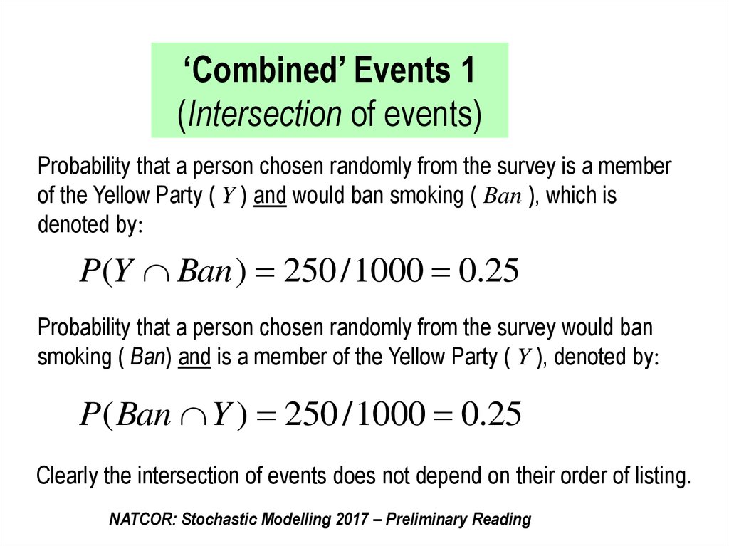
‘Combined’ Events 1
(Intersection of events)
Probability that a person chosen randomly from the survey is a member
of the Yellow Party ( Y ) and would ban smoking ( Ban ), which is
denoted by:
P(Y Ban ) 250 / 1000 0.25
Probability that a person chosen randomly from the survey would ban
smoking ( Ban) and is a member of the Yellow Party ( Y ), denoted by:
P( Ban Y ) 250 / 1000 0.25
Clearly the intersection of events does not depend on their order of listing.
NATCOR: Stochastic Modelling 2017 – Preliminary Reading

8.

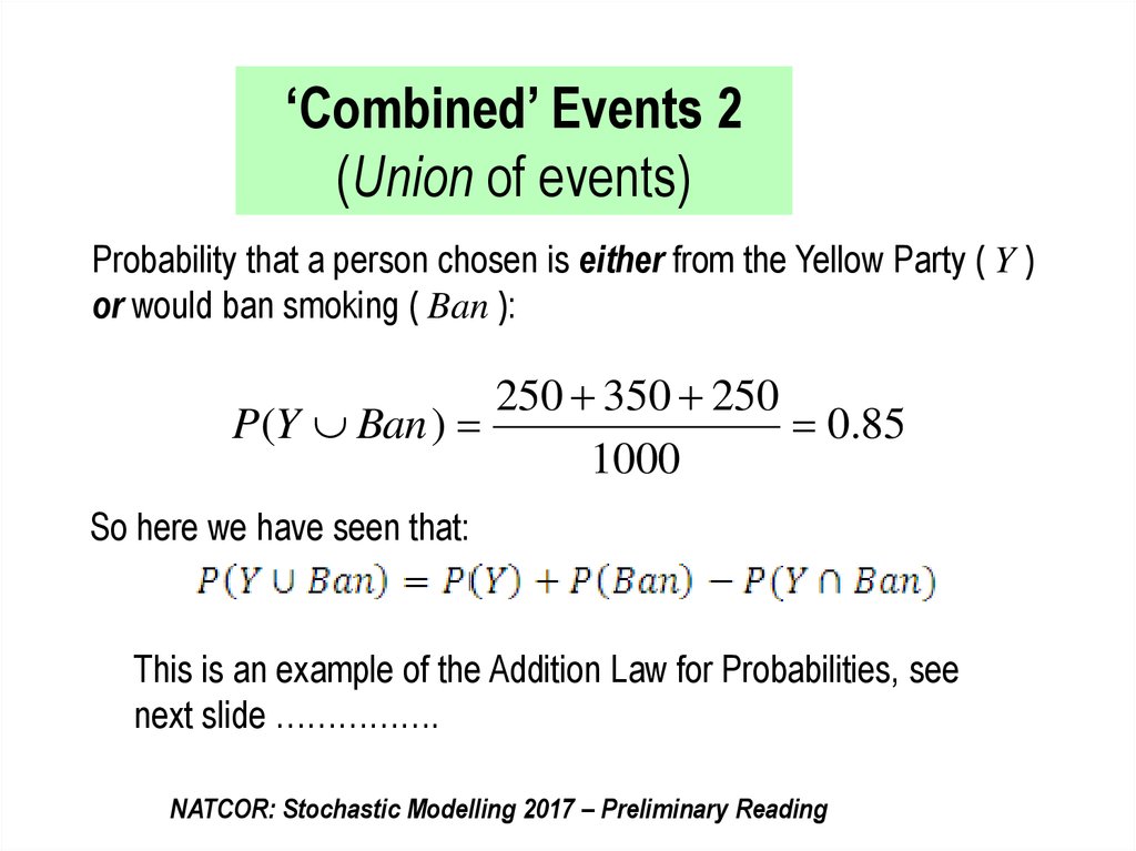
‘Combined’ Events 2
(Union of events)
Probability that a person chosen is either from the Yellow Party ( Y )
or would ban smoking ( Ban ):
250 350 250
P(Y Ban )
0.85
1000
So here we have seen that:
This is an example of the Addition Law for Probabilities, see
next slide …………….
NATCOR: Stochastic Modelling 2017 – Preliminary Reading

9.

Addition Law for Probabilities (in general):
P( A B) P( A) P( B) P( A B)
A special case is when Events A and B are mutually exclusive ,
i.e. they cannot both happen, in which case the addition law
simplifies to:
P( A B) P( A) P( B)
NATCOR: Stochastic Modelling 2017 – Preliminary Reading

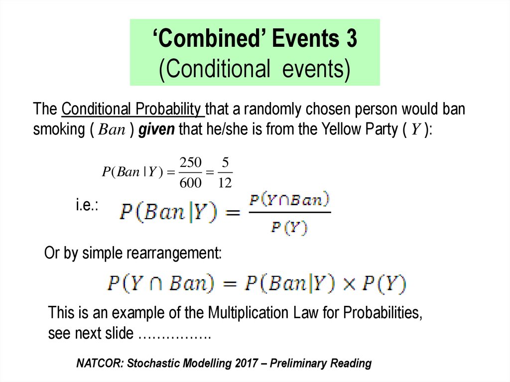
10.

‘Combined’ Events 3
(Conditional events)
The Conditional Probability that a randomly chosen person would ban
smoking ( Ban ) given that he/she is from the Yellow Party ( Y ):
P( Ban | Y )
250 5
600 12
i.e.:
Or by simple rearrangement:
This is an example of the Multiplication Law for Probabilities,
see next slide …………….
NATCOR: Stochastic Modelling 2017 – Preliminary Reading

11.

Multiplication Law for Probabilities (in general)
P( B A)
P( B / A)
P( A)
or
P( B A) P( B / A) P( A)
A special case is when Events A and B are independent,
i.e. the occurrence of A has no influence on the probability
of B [and vice versa)]
i.e. P(B/A) = P(B) [and P(A/B)=P(A)]
in which case the multiplication law simplifies to:
P( B A) P( B) P( A)
NOTE: This notion of independence can be extended to more than 2 events.
NATCOR: Stochastic Modelling 2017 – Preliminary Reading

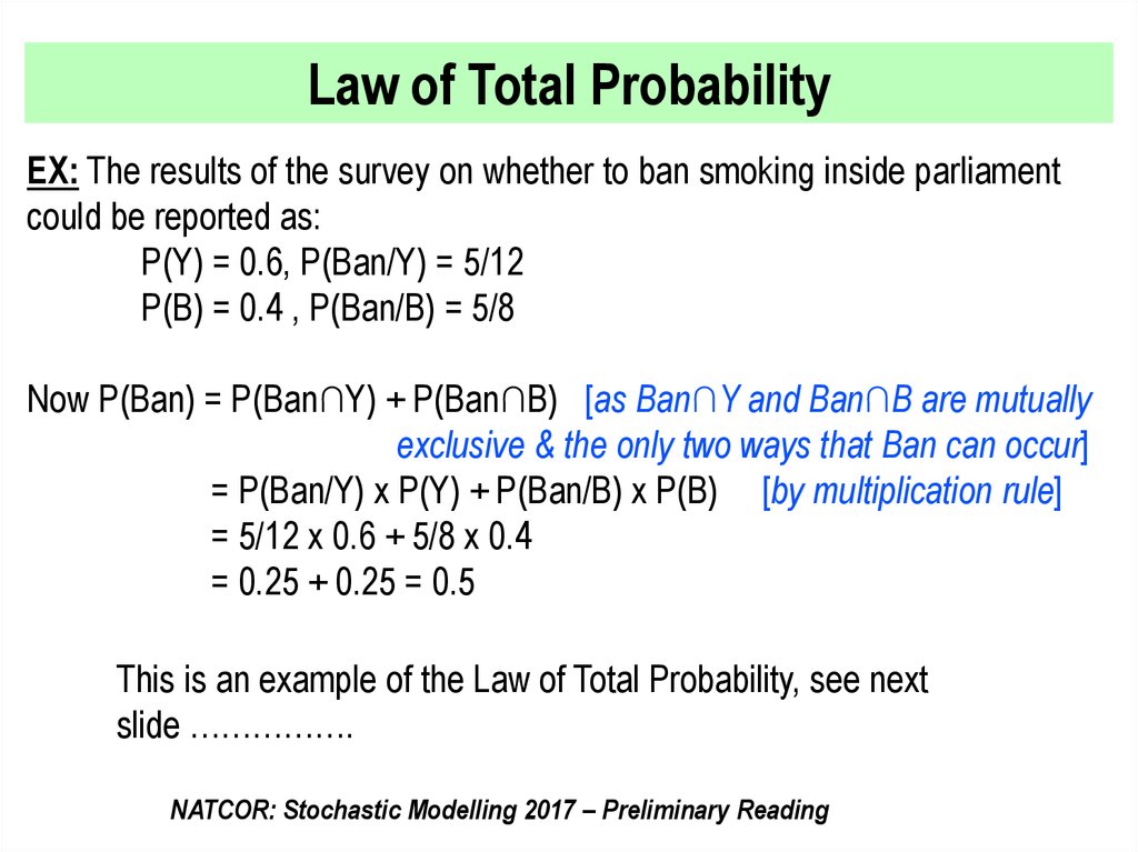
12.

Law of Total Probability
EX: The results of the survey on whether to ban smoking inside parliament
could be reported as:
P(Y) = 0.6, P(Ban/Y) = 5/12
P(B) = 0.4 , P(Ban/B) = 5/8
Now P(Ban) = P(Ban∩Y) + P(Ban∩B) [as Ban∩Y and Ban∩B are mutually
exclusive & the only two ways that Ban can occur]
= P(Ban/Y) x P(Y) + P(Ban/B) x P(B) [by multiplication rule]
= 5/12 x 0.6 + 5/8 x 0.4
= 0.25 + 0.25 = 0.5
This is an example of the Law of Total Probability, see next
slide …………….
NATCOR: Stochastic Modelling 2017 – Preliminary Reading

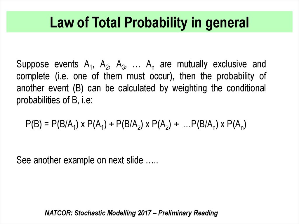
13.

Law of Total Probability in general
Suppose events A1, A2, A3, … An are mutually exclusive and
complete (i.e. one of them must occur), then the probability of
another event (B) can be calculated by weighting the conditional
probabilities of B, i.e:
P(B) = P(B/A1) x P(A1) + P(B/A2) x P(A2) + …P(B/An) x P(An)
See another example on next slide …..
NATCOR: Stochastic Modelling 2017 – Preliminary Reading

14.

Tree Diagrams also help think about probabilities
In a factory, a brand of chocolates is
packed into boxes on four production
lines A, B, C, D. Records show that
a small percentage of boxes are not
packed properly for sale as follows
Line
A
B
C
D
% Faulty
1
3
2.5
2
% Output
35
20
24
21
What is the probability that a box
chosen at random from the factory’s
output is faulty?
NATCOR: Stochastic Modelling 2017 – Preliminary Reading

15. Discrete Random Variables

• A random variable is a numerical description of the
outcome of an experiment.
• When the values are ‘discrete’, (e.g. value shown
when die is thrown, first number drawn in lottery,
daily number of patients attending A&E in
Lancaster), the random variable is discrete.
• { For Later ***When the values are ‘continuous’ ,
(e.g. height of randomly selected student,
temperature in Lancaster, time between patients
arriving at A&E), the random variable is continuous.}
NATCOR: Stochastic Modelling 2013 – Preliminary Reading
•LUMS: Dept of Management Science Masters Programmes 2008/9: ASWFS – Chap 5

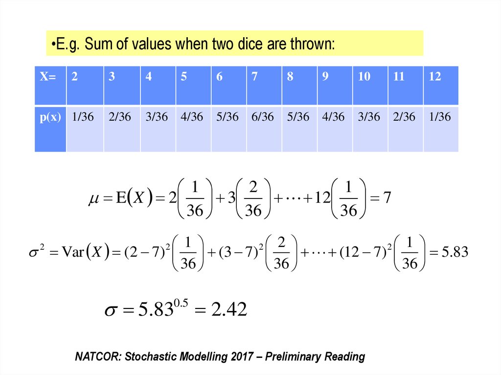
16. Probability Mass Function (pmf) of a discrete random variable

•The pmf, p(x), of a discrete random variable (X) simply lists the
probabilities of each possible value, x, of the random variable.
•E.g. Sum of values when two dice are thrown:
X=
2
p(x) 1/36
3
4
5
6
7
8
9
10
11
12
2/36
3/36
4/36
5/36
6/36
5/36
4/36
3/36
2/36
1/36
NATCOR: Stochastic Modelling 2017 – Preliminary Reading

17. Expected value and variance of discrete random variables

•The expected value, or mean, of a discrete random
variable is defined as:
•The variance of a discrete random variable is a measure of
variability and is defined as:
•N.B. σ is referred to as the standard deviation of X.
NATCOR: Stochastic Modelling 2017 – Preliminary Reading

18.

•E.g. Sum of values when two dice are thrown:
X=
2
p(x) 1/36
3
4
5
6
7
8
9
10
11
12
2/36
3/36
4/36
5/36
6/36
5/36
4/36
3/36
2/36
1/36
1 2
1
3
12
7
36 36
36
E X 2
1
2 2
2 1
Var X (2 7) (3 7) (12 7) 5.83
36
36
36
2
2
5.830.5 2.42
NATCOR: Stochastic Modelling 2017 – Preliminary Reading

19. Expected value and variance of combinations of discrete random variables

•If X and Y are random variables and a and b are constants:
E(aX + bY) = aE(X) + bE(Y);
•If X and Y are also independent random variables (i.e. the value of
X has no influence on the value of Y (e.g. two throws of a die))
E(XY) = E(X)E(Y)
and
Var (aX + bY) = a2 Var(X) + c2 Var(Y).
NATCOR: Stochastic Modelling 2017 – Preliminary Reading

20.

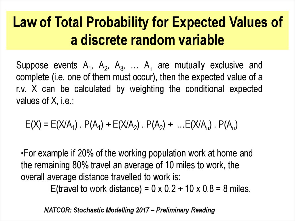
Law of Total Probability for Expected Values of
a discrete random variable
Suppose events A1, A2, A3, … An are mutually exclusive and
complete (i.e. one of them must occur), then the expected value of a
r.v. X can be calculated by weighting the conditional expected
values of X, i.e.:
E(X) = E(X/A1) . P(A1) + E(X/A2) . P(A2) + …E(X/An) . P(An)
•For example if 20% of the working population work at home and
the remaining 80% travel an average of 10 miles to work, the
overall average distance travelled to work is:
E(travel to work distance) = 0 x 0.2 + 10 x 0.8 = 8 miles.
NATCOR: Stochastic Modelling 2017 – Preliminary Reading

21. Poisson Random Variable

• The most important
discrete random variable in
stochastic modelling is the
Poisson random variable.
e.g. p(x) for Poisson r.v. with
=3.5
0,250
0,200
0,150
• A Poisson distribution
with mean has pmf:
e x
p( x )
x!
and its variance 2 = .
0,100
0,050
0,000
0
1
2
3
4
5
6
7
8
9
10
•And Poisson probabilities
can be obtained directly from
the formula, statistical tables
or computer software.
NATCOR: Stochastic Modelling 2017 – Preliminary Reading

22. Poisson Random Variable

The General Theory:
When ‘events’ of interest occur ‘at random’ at rate l
per unit time;
No. of events in period of time T has a Poisson
distribution with mean lT
Events in real stochastic processes (e.g. arrivals of
customers at a bank, calls to a call centre, patients to
an A&E department, breakdowns in equipment) occur
‘at random’ when there are a large number of potential
customers/ callers/ patients/ components each with
independent probabilities of arriving/ calling/ falling ill/
breaking.
NATCOR: Stochastic Modelling 2017 – Preliminary Reading

23. Poisson Random Variable

Example:
If arrivals of customers to
a bank are at random, at
an average rate of 0.6
per minute, then:
No. of arrivals in 5
minute period has
Poisson distribution with
mean = 3.
x
0
1
2
3
4
5
6
7
8
9
……
p(x)
0.050
0.149
0.224
0.224
0.168
0.101
0.050
0.022
0.008
0.003
……
0,250
0,200
0,150
0,100
0,050
0,000
0
1
2
NATCOR: Stochastic Modelling 2017 – Preliminary Reading
3
4
5
6
7
8
9
10

24. Continuous Random Variables

• A random variable is a numerical description of the
outcome of an experiment.
• When the values are ‘continuous’ , (e.g. height of
randomly selected student, temperature in
Lancaster, time between patients arriving at A&E),
the random variable is continuous.
NATCOR: Stochastic Modelling 2017 – Preliminary Reading

25.

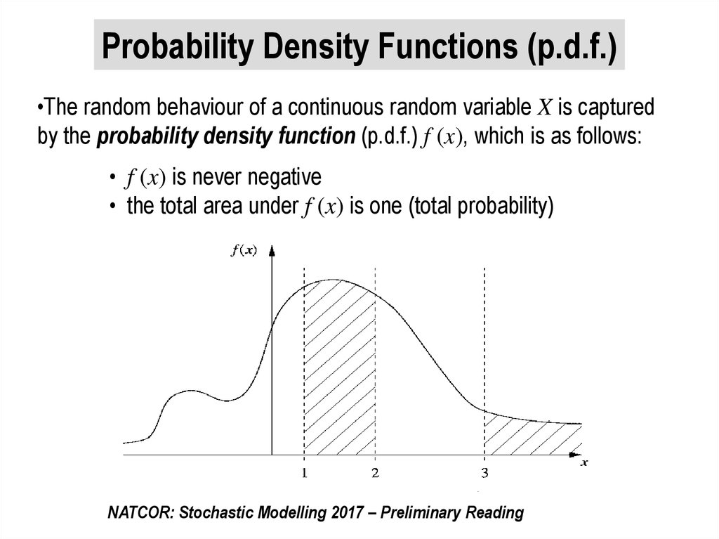
Probability Density Functions (p.d.f.)
•The random behaviour of a continuous random variable X is captured
by the probability density function (p.d.f.) f (x), which is as follows:
• f (x) is never negative
• the total area under f (x) is one (total probability)
NATCOR: Stochastic Modelling 2017 – Preliminary Reading

26.

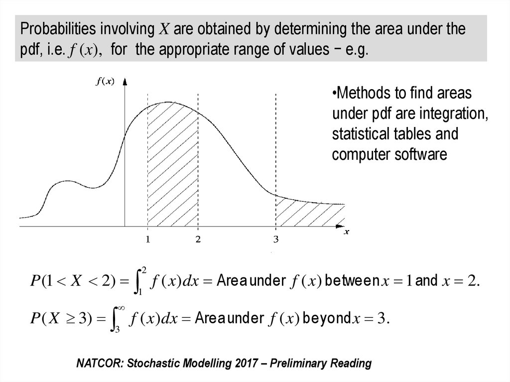
Probabilities involving X are obtained by determining the area under the
pdf, i.e. f (x), for the appropriate range of values − e.g.
•Methods to find areas
under pdf are integration,
statistical tables and
computer software
2
P (1 X 2) f ( x)dx Area under f ( x ) between x 1 and x 2.
1
P ( X 3) f ( x)dx Area under f ( x) beyond x 3.
3
NATCOR: Stochastic Modelling 2017 – Preliminary Reading

27. Expected value and variance of continuous random variables

•The expected value, or mean, of a continuous random
variable is defined as:
E X xf x dx
•The variance of a continuous random variable is a measure
of variability and is defined as:
Var X E X
2
2
x f x dx
2
•N.B. σ is referred to as the standard deviation of X.
NATCOR: Stochastic Modelling 2017 – Preliminary Reading

28. Expected value and variance of combinations of continuous random variables NB. Exactly same as for discrete r.v.

•If X and Y are random variables and a and b are constants:
E(aX + bY) = aE(X) + bE(Y);
•If X and Y are also independent random variables (i.e. the value of
X has no influence on the value of Y (e.g. two throws of a die))
E(XY) = E(X)E(Y)
and
Var (aX + bY) = a2 Var(X) + c2 Var(Y).
NATCOR: Stochastic Modelling 2017 – Preliminary Reading

29.

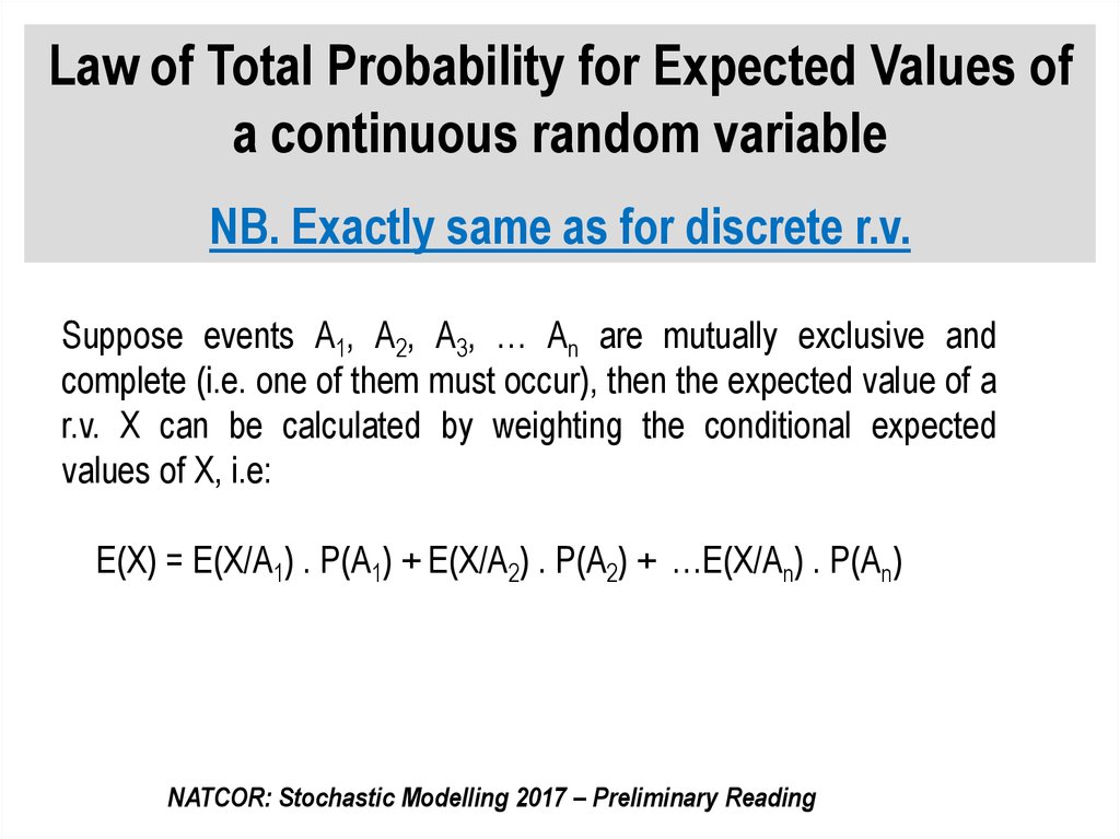
Law of Total Probability for Expected Values of
a continuous random variable
NB. Exactly same as for discrete r.v.
Suppose events A1, A2, A3, … An are mutually exclusive and
complete (i.e. one of them must occur), then the expected value of a
r.v. X can be calculated by weighting the conditional expected
values of X, i.e:
E(X) = E(X/A1) . P(A1) + E(X/A2) . P(A2) + …E(X/An) . P(An)
NATCOR: Stochastic Modelling 2017 – Preliminary Reading

30. Exponential Random Variable

• The most important
continuous random variable
in stochastic modelling is
the Exponential random
variable.
• Exponential distribution
with mean 1/g has pdf:
E.g. f(x) for Exponential r.v.
with mean=4.
0,3
0,25
0,2
0,15
0,1
0,05
0
0
f(x) ge gx
2
4
6
8
10
12
•And areas under curve
follow from simple formula:
• and its variance 2 = (1/g 2,
i.e. variance = mean2
NATCOR: Stochastic Modelling 2017 – Preliminary Reading
14

31. Exponential Random Variable

The General Theory:
When ‘events’ of interest occur ‘at random’ at rate l per unit time
(as is common in real stochastic processes – see earlier note);
The time between events has an Exponential distribution with
mean 1/l.
And the time to the next event has an Exponential distribution
with mean 1/l, whether or not an event has just occurred. [This is
the memoryless property of the Exponential distribution – and is
counter-intuitive!].
Conversely, if the gaps between events are independent and
from an exponential distribution with mean 1/l, the events occur
‘at random’ at rate l per unit time.
NATCOR: Stochastic Modelling 2017 – Preliminary Reading

32. Exponential Example

THEORY
• IF Events occur ‘at random’, at
rate A per unit time.
EXAMPLE
• IF Arrivals to bank occur ‘at
random’, at rate of 0.6 per minute.
THEN: Time between events has
an Exponential distribution, with
mean of 1/A.
THEN: Time between arrivals has
an Exponential distribution, with
mean = 1.667 minutes.
AND: Time to next event has an
Exponential distribution, with
mean of 1/A.
AND: Time to next arrival has an
Exponential distribution, with
mean of 1.667 minutes.
NATCOR: Stochastic Modelling 2017 – Preliminary Reading

33. Normal Random Variable

• The most important
continuous random variable
in statistics is the Normal
random variable.
E.g. f(x) for Normal r.v. with
mean= and stan dev ..
Point of
inflection
• Normal distribution with
mean and variance 2
has pdf:
f(x)
1
2
e
[ ( x ) 2 2 2 ]
& hence its standard deviation
is .
•And areas under curve are
obtained from statistical tables
or from computer software.
NATCOR: Stochastic Modelling 2017 – Preliminary Reading

34. Standardised Normal Random Variable

•Areas under any Normal curve
(mean= & SD= )
can be found by finding the
‘equivalent’ area under the
standard Normal curve
(mean=0 & SD=1), i.e.:
SD=
a
b
X
SD =1
(a- /
NATCOR: Stochastic Modelling 2017 – Preliminary Reading
0
(b- / Z

35. Normal Random Variables

Important (in general) because:
• Many naturally occurring r.v.’s have a Normal
distribution, e.g. weights, heights …
• Many useful statistics behave as Normal r.v.’s,
even if the r.v.’s from which they derive are not
Normal, e.g. Central Limit Theorem.
NATCOR: Stochastic Modelling 2017 – Preliminary Reading