Discrete Probability Distributions: Binomial and Poisson Distribution. Week 7 (2)

1. BBA182 Applied Statistics Week 7 (2) Discrete Probability Distributions: Binomial and Poisson Distribution

DR SUSANNE HANSEN SARAL
EMAIL: [email protected]
HT TPS://PIAZZA.COM/CLASS/IXRJ5MMOX1U2T8?CID=4#
WWW.KHANACADEMY.ORG
DR SUSANNE HANSEN SARAL
1

2. Mid-term exam

Bring:
• Calculator
•Pen
•Eraser
23/03/2017
11:45 – 13:00 hours

3. Probability and cumulative probability distribution of a discrete random variable

In the last class we saw how to calculate the probability
of a specific discrete random variable, such as P( x = 3)
and the cumulative probability such as P(x ≥ 3) in n trials
with the following formula:
We need to know n, x and P (probability of success)

4. The binomial distribution is used to find the probability of a specific or cumulative number of successes in n trials.

NUMBER OF
HEADS (r)
PROBABILITY =
0
P(X = 0)
0.0778 =
1
P(X = 1)
0.2592 =
2
P(X = 2)
0.3456 =
3
P(X = 3)
0.2304 =
4
P(X = 4)
0.0768 =
5
P(X = 5)
0.0102 =
5!
(0.5)r(0.5)5 – r
r!(5 – r)!
5!
0!(5 – 0)!
5!
1!(5 – 1)!
5!
2!(5 – 2)!
5!
3!(5 – 3)!
5!
4!(5 – 4)!
5!
5!(5 – 5)!
DR SUSANNE HANSEN SARAL
(0.5)0(0.5)5 – 0
(0.5)1(0.5)5 – 1
(0.5)2(0.5)5 – 2
(0.5)3(0.5)5 – 3
(0.5)4(0.5)5 – 4
(0.5)5(0.5)5 – 5
4

5. Probability and cumulative probability distribution of a discrete random variable

Ali, real estate agent has 5 potential customers to buy a house or apartment with a
probability of 0.40. The probability and cumulative probability table of the sale of
houses here below. We are able to answer what is P( x=3), P(x ≤ 4), P(x >3)etc.

6. Shape of Binomial Distribution

Mean
The shape of the binomial distribution depends on the
values of P and n
Here, n = 5 and P = 0.1
.6
.4
.2
0
P(x)
x
0
Here, n = 5 and P = 0.5
.6
.4
.2
0
n = 5 P = 0.1
P(x)
2
3
4
5
n = 5 P = 0.5
x
0
DR SUSANNE HANSEN SARAL
1
1
2
3
4
5
Ch. 4-6

7. Binomial Distribution shapes

When P = .5 the shape of the distribution is perfectly symmetrical and
resembles a bell-shaped (normal distribution)
When P = .2 the distribution is skewed right. This skewness increases as P
becomes smaller.
When P = .8, the distribution is skewed left. As P comes closer to 1, the
amount of skewness increases.
DR SUSANNE HANSEN SARAL
7

8. Using Binomial Tables instead of to calculating Binomial probabilities manually

N
x
…
p=.20
p=.25
p=.30
p=.35
p=.40
p=.45
p=.50
10
0
1
2
3
4
5
6
7
8
9
10
…
…
…
…
…
…
…
…
…
…
…
0.1074
0.2684
0.3020
0.2013
0.0881
0.0264
0.0055
0.0008
0.0001
0.0000
0.0000
0.0563
0.1877
0.2816
0.2503
0.1460
0.0584
0.0162
0.0031
0.0004
0.0000
0.0000
0.0282
0.1211
0.2335
0.2668
0.2001
0.1029
0.0368
0.0090
0.0014
0.0001
0.0000
0.0135
0.0725
0.1757
0.2522
0.2377
0.1536
0.0689
0.0212
0.0043
0.0005
0.0000
0.0060
0.0403
0.1209
0.2150
0.2508
0.2007
0.1115
0.0425
0.0106
0.0016
0.0001
0.0025
0.0207
0.0763
0.1665
0.2384
0.2340
0.1596
0.0746
0.0229
0.0042
0.0003
0.0010
0.0098
0.0439
0.1172
0.2051
0.2461
0.2051
0.1172
0.0439
0.0098
0.0010
Examples:
n = 10, x = 3, P = 0.35:
P(x = 3|n =10, p = 0.35) = .2522
n = 10, x = 8, P = 0.45:
P(x = 8|n =10, p = 0.45) = .0229
DR SUSANNE HANSEN SARAL
Ch. 4-8

9. Solving Problems with Binomial Tables

MSA Electronics is experimenting with the manufacture of a new
USB-stick and is looking into the number of defective USB-sticks
◦ Every hour a random sample of 5 USB-sticks is taken
◦ The probability of one USB-stick being defective is 0.15
◦ What is the probability of finding 3, 4, or 5 defective USB-sticks ?
P( x = 3), P(x = 4 ), P(x= 5)
n = 5, p = 0.15, and r = 3, 4, or 5
DR SUSANNE HANSEN SARAL
2–9

10. Solving Problems with Binomial Tables

TABLE 2.9 (partial) – Table for Binomial Distribution, n= 5,
n
5
r
0
1
2
3
4
5
0.05
0.7738
0.2036
0.0214
0.0011
0.0000
0.0000
P
0.10
0.5905
0.3281
0.0729
0.0081
0.0005
0.0000
DR SUSANNE HANSEN SARAL
0.15
0.4437
0.3915
0.1382
0.0244
0.0022
0.0001
2 – 10

11. Solving Problems with Binomial Tables

MSA Electronics is experimenting with the manufacture of a new
USB-stick
◦ Every hour a random sample of 5 USB-sticks is taken
◦ The probability of one USB-stick being defective is 0.15
◦ What is the probability of finding more than 3 (3 inclusive) defective USBsticks? P( x ≥ 3)
n = 5, p = 0.15, and r = 3, 4, or 5
DR SUSANNE HANSEN SARAL
2 – 11

12. Solving Problems with Binomial Tables Cumulative probability

TABLE 2.9 (partial) – Table for Binomial Distribution
n
5
r
0
1
2
3
4
5
0.05
0.7738
0.2036
0.0214
0.0011
0.0000
0.0000
P
0.10
0.5905
0.3281
0.0729
0.0081
0.0005
0.0000
0.15
0.4437
0.3915
0.1382
0.0244
0.0022
0.0001
We find the three probabilities in the table for
n = 5, p = 0.15, and r = 3, 4, and 5 and add
them together
DR SUSANNE HANSEN SARAL
2 – 12

13. Solving Problems with Binomial Tables Cumulative probabilities

TABLE 2.9 (partial) – Table for Binomial Distribution
n
0.05
P(3
orr more defects)
=
5
0
1
2
3
4
5
0.7738
0.2036
0.0214
0.0011
0.0000
0.0000
=
=
P
P(3)0.10
+ P(4) + P(5) 0.15
0.5905
0.4437
0.0244
0.0001
0.3281+ 0.0022 +
0.3915
0.0729
0.1382
0.0267
0.0081
0.0244
0.0005
0.0022
0.0000
0.0001
We find the three probabilities in the table for n =
5, p = 0.15, and r = 3, 4, and 5 and add them
together
DR SUSANNE HANSEN SARAL
2 – 13

14. Suppose that Ali, a real estate agent, has 10 people interested in buying a house. He believes that for each of the 10 people the probability of selling a house is 0.40. What is the probability that he will sell 4 houses, P(x = 4)?

DR SUSANNE HANSEN SARAL
14

15. Suppose that Ali, a real estate agent, has 10 people interested in buying a house. He believes that for each of the 10 people the probability of selling a house is 0.40. What is the probability that he will sell 4 houses?

DR SUSANNE HANSEN SARAL
15

16. Suppose that Ali, a real estate agent, has 10 people interested in buying a house. He believes that for each of the 10 people the probability of selling a house is 0.20. What is the probability that he will sell 7 houses, P(x = 7)?

DR SUSANNE HANSEN SARAL
16

17. Suppose that Ali, a real estate agent, has 10 people interested in buying a house. He believes that for each of the 10 people the probability of selling a house is 0.35. What is the probability that he will sell more than 7 houses, 7 houses included, P(x

Suppose that Ali, a real estate agent, has 10 people interested in buying a
house. He believes that for each of the 10 people the probability of selling
a house is 0.35. What is the probability that he will sell more than 7
houses, 7 houses included, P(x ≥ 7)?
DR SUSANNE HANSEN SARAL
17

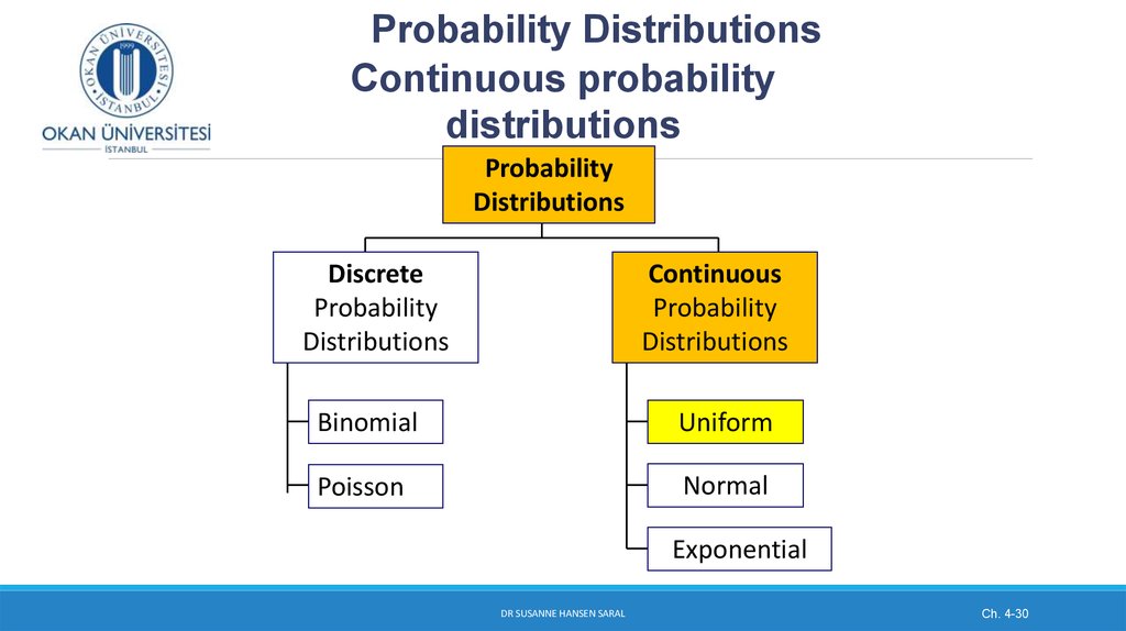
18.

Probability Distributions
Probability
Distributions
Discrete
Probability
Distributions
Continuous
Probability
Distributions
Binomial
Uniform
Poisson
Normal
Exponential
DR SUSANNE HANSEN SARAL
Ch. 4-18

19. Poisson random variable, first proposed by Frenchman Simeon Poisson (1781-1840)

A Poisson distributed random variable is often
useful in estimating the number of occurrences
over a specified interval of time or space.
It is a discrete random variable that may assume
an infinite sequence of values (x = 0, 1, 2, . . . ).
DR SUSANNE HANSEN SARAL
19

20. Poisson Random Variable - three requirements

Poisson Random Variable three requirements
1. The number of expected outcomes in one interval of time or unit space
is unaffected (independent) by the number of expected outcomes in any
other non-overlapping time interval.
Example: What took place between 3:00 and 3:20 p.m. is not affected by
what took place between 9:00 and 9:20 a.m.
DR SUSANNE HANSEN SARAL
20

21. Poisson Random Variable - three requirements (continued)

Poisson Random Variable three requirements (continued)
2.The expected (or mean) number of outcomes over any time period or unit space is
proportional to the size of this time interval.
Example:
We expect half as many outcomes between 3:00 and 3:30 P.M. as between 3:00 and 4:00
P.M.
3.This requirement also implies that the probability of an occurrence must be constant over any
intervals of the same length.
Example:
The expected outcome between 3:00 and 3:30P.M. is equal to the expected occurrence
between 4:00 and 4:30 P.M..
DR SUSANNE HANSEN SARAL
21

22. Examples of a Poisson Random variable

The number of cars arriving at a toll booth in 1 hour (the time interval is 1 hour)
The number of failures in a large computer system during a given day (the given day is
the interval)
The number of delivery trucks to arrive at a central warehouse in an hour.
The number of customers to arrive for flights at an airport during each 10-minute time
interval from 3:00 p.m. to 6:00 p.m. on weekdays
DR SUSANNE HANSEN SARAL
22

23. Situations where the Poisson distribution is widely used: Capacity planning – time interval

Areas of capacity planning observed in a sample:
A bank wants to know how many customers arrive at the bank in a given time period
during the day, so that they can anticipate the waiting lines and plan for the number of
employees to hire.
At peak hours they might want to open more guichets (employ more personnel) to
reduce waiting lines and during slower hours, have a few guichets open (need for less
personnel).
DR SUSANNE HANSEN SARAL
23

24. Poisson Probability Distribution

Poisson Probability Function