 Random variables – discrete random variables")


 for Discrete Random Variables")
 for Discrete Random Variables (example)")


")
")
 Cumulative probability distribution, Ogive")
 Practical application")
 Practical application: Car dealer")
 Practical application")
 Practical application")


")


 mathematics
Similar presentations:
")
. Week 2 (2)")
")
")


")
")
")
")
Random variables – discrete random variables. Week 6 (2)
1. BBA182 Applied Statistics Week 6 (2) Random variables – discrete random variables
DR SUSANNE HANSEN SARALEMAIL: SUSANNE.SARAL@OKAN.EDU.TR
HT TPS://PIAZZA.COM/CLASS/IXRJ5MMOX1U2T8?CID=4#
WWW.KHANACADEMY.ORG
DR SUSANNE HANSEN SARAL
1
2. Random Variables
Represent possible numerical values from a random experiments. Whichoutcome will occur, is not known, therefore the word “random”.
Random
Variables
Discrete
Random Variable
Continuous
Random Variable
DR SUSANNE HANSEN SARAL
Ch. 4-2
3. Discrete random variable
A discrete random variable is a possible outcome from a random experiment.It takes on countable values, integers.
Examples of discrete random variables:
Number of cars crossing the Bosphorus Bridge every day
Number of journal subscriptions
Number of visits on a given homepage per day
We can calculate the exact probability of a discrete random variable:
4. Discrete random variable
We can calculate the exact probability of a discrete random variable.Example: The probability of students coming late to class today out of all students
registered
Total students registered: 45
Students late for the class: 15
P(students late for the class) =
15
45
= .33 or 33 %
5. Continuous random variable
A random variable that has an unlimited set of values. Therefore called continuous random variableContinuous random variables are common in business applications for modeling physical
quantities such as height, volume and weight, and monetary quantities such as profits, revenues
and expenses.
Examples:
The weight of cereal boxes filled by a filling machine in grams
Air temperature on a given summer day in degrees Celsius
Height of a building in meters
Annual profits in $ of 10 Turkish companies
6. Continuous random variable
A continuous random variable has an unlimited set of values.The probability of a continuous variable is calculated in an interval (ex.: 5 -10), because the
probability of a specific continuous random variable is close to 0. This would not provide
useful information.
Example: The time it takes for each of 110 employees in a factory to assemble a toaster:
7. Time, in seconds, it takes 110 employees to assemble a toaster
271 236 294 252 254 263 266 222 262 278 288262 237 247 282 224 263 267 254 271 278 263
262 288 247 252 264 263 247 225 281 279 238
252 242 248 263
263 242 288
255 294 268 255 272 271 291
252 226 263 269 227 273 281 267
263 244
249 252 256 263 252 261 245 252 294
288 245
251 269 256 264 252 232 275 284 252
263 274
252
252 256 254 269 234 285 275 263
263 246
294
252 231 265 269 235
275 288 294
269
276 248 299
263 247 252
261 266 269 236
DR SUSANNE HANSEN SARAL, SUSANNE.SARAL@GMAIL.COM
8. Continuous random variable
The probability of a continuous variable is calculated in an interval (5 - 10), because the probability of aspecific continuous random variable is close to 0.
Example: The time it takes for each of 110 employees in a factory to assemble a toaster:
n = 110
1 employee assembles the toaster is 222 seconds out of 110
P(employee assembles the toaster in 222 seconds out of all 110 employees) =
this provides little useful information
1
110
= 0.009 or 0.9 %
9. Employee assembly time in seconds
Completion time (in seconds)Frequency
Relative frequency %
220 – 229
5
4.5
230 – 239
8
7.3
240 – 249
13
11.8
250 – 259
22
20.0
260 – 269
32
29.1
270 – 279
13
11.8
280 – 289
10
9.1
290 – 300
7
6.4
Total
110
DR SUSANNE HANSEN SARAL, SUSANNE.SARAL@GMAIL.COM
100 %
10. Probability Models
For both discrete and continuous variables, the collection of all possible outcomes (samplespace) and probabilities associated with them is called the probability model.
For a discrete random variable, we can list the probability of all possible values in a table.
For example, to model the possible outcomes of a dice, we let X be the random variable
called the “number showing on the face of the dice”. The probability model for X is therefore:
1/6
if x = 1, 2, 3, 4, 5, or 6
P(X = x) =
0 otherwise
11.
Probability Model forDiscrete Random Variables
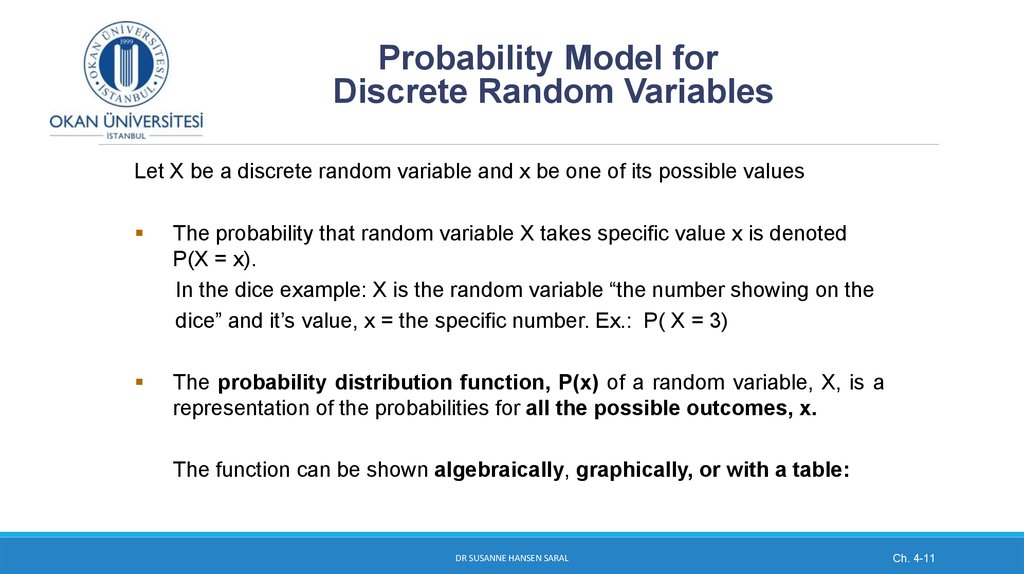
Let X be a discrete random variable and x be one of its possible values
The probability that random variable X takes specific value x is denoted
P(X = x).
In the dice example: X is the random variable “the number showing on the
dice” and it’s value, x = the specific number. Ex.: P( X = 3)
The probability distribution function, P(x) of a random variable, X, is a
representation of the probabilities for all the possible outcomes, x.
The function can be shown algebraically, graphically, or with a table:
DR SUSANNE HANSEN SARAL
Ch. 4-11
12. Probability Model, also Probability Distributions Function, P(x) for Discrete Random Variables
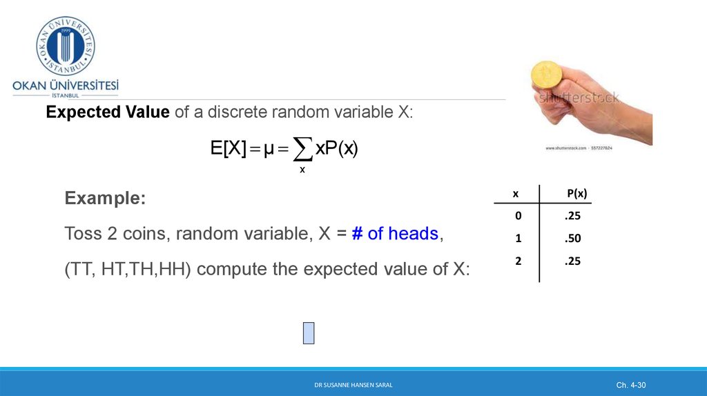
Experiment: Toss 2 Coins simultaneously. Let the random variable, X, be the #heads
4 possible outcomes
(values for x)
Probability Distribution
T
T
H
H
T
H
H
0
1/4 = .25
1
2/4 = .50
2
1/4 = .25
Probability
T
.50
.25
0
DR SUSANNE HANSEN SARAL
1
2
Ch. 4-12
x
13. Probability Distributions Function, P(x) for Discrete Random Variables (example)
Sales of sandwiches in a sandwich shop:Let, the random variable X, represent the number of sandwiches
sold within the time period of 14:00 - 16:00 hours in one given day.
The probability distribution function, P(x) of sales is given by the
table here below:
x
0
1
2
3
Total
P(x)
0.1
0.2
0.4
0.3
1.00
DR SUSANNE HANSEN SARAL
13
14. Graphical illustration of the probability distribution of sandwich sales between 14:00 -16:00 hours
DR SUSANNE HANSEN SARAL14
15. Requirements for a probability distribution of a discrete random variable
1. 0 ≤ P(x) ≤ 1 for any value of x2. The individual probabilities of all outcomes sum up to 1;
P(x) 1
x
All possible values of X are mutually exclusive and collectively exhaustive (the
outcomes make up the entire sample space), therefore the probabilities for
these events must sum to 1.
DR SUSANNE HANSEN SARAL
Ch. 4-15
16. Cumulative Probability Function
(continued)Example: Toss 2 coins simultaneously
Let the random variable, X, be number of the heads. There are 4 possible
outcomes:
X Value
P(x)
F(x)
0
0.25
0.25
1 (x2)
0.50
0.75
2
0.25
1.00
F(x0) =