Probabilities. Week 5 (2)

1. BBA182 Applied Statistics Week 5 (2) Probabilities

DR SUSANNE HANSEN SARAL
EMAIL: [email protected]
HT TPS://PIAZZA.COM/CLASS/IXRJ5MMOX1U2T8?CID=4#
WWW.KHANACADEMY.ORG
DR SUSANNE HANSEN SARAL
1

2. Where do probabilities come from?

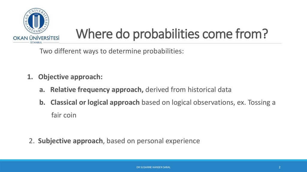
Two different ways to determine probabilities:
1. Objective approach:
a. Relative frequency approach, derived from historical data
b. Classical or logical approach based on logical observations, ex. Tossing a
fair coin
2. Subjective approach, based on personal experience
DR SUSANNE HANSEN SARAL
2

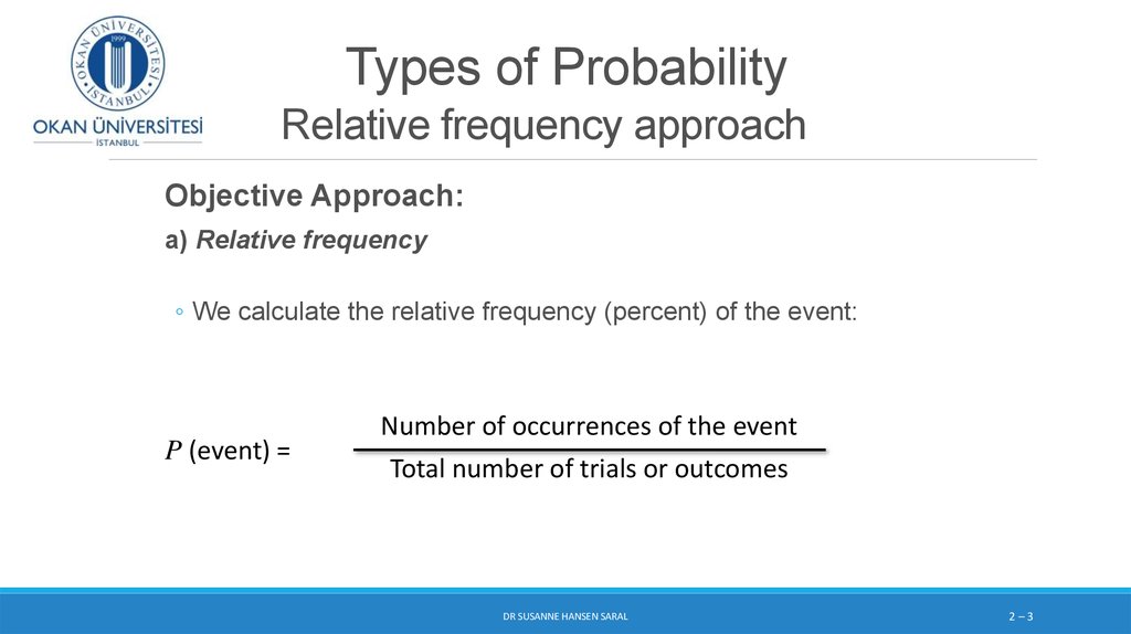
3. Types of Probability Relative frequency approach

Objective Approach:
a) Relative frequency
◦ We calculate the relative frequency (percent) of the event:
P (event) =
Number of occurrences of the event
Total number of trials or outcomes
DR SUSANNE HANSEN SARAL
2–3

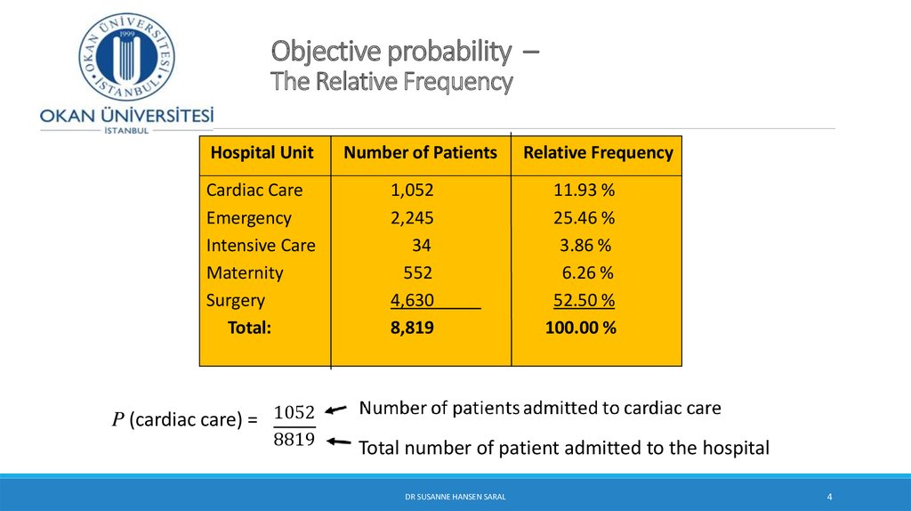
4. Objective probability – The Relative Frequency

Hospital Unit
Cardiac Care
Emergency
Intensive Care
Maternity
Surgery
Total:
Number of Patients
1,052
2,245
34
552
4,630
8,819
Relative Frequency
11.93 %
25.46 %
3.86 %
6.26 %
52.50 %
100.00 %
P (cardiac care) = 1052
8819
Total number of patient admitted to the hospital
DR SUSANNE HANSEN SARAL
4

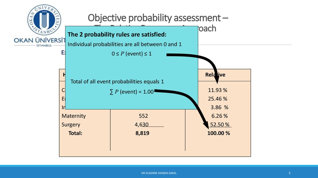
5. Objective probability assessment – The Relative Frequency Approach

The 2 probability rules are satisfied:
Individual probabilities are all between 0 and 1
Example: Hospital 0Patients
by ≤Unit
≤ P (event)
1 per semester
Hospital Unit
Number of Patients
Total of
all event probabilities equals 1
Frequency
Cardiac Care
∑ P (event)1,052
= 1.00
Emergency
2,245
Intensive Care
340
Maternity
552
Surgery
4,630
Total:
8,819
DR SUSANNE HANSEN SARAL
Relative
11.93 %
25.46 %
3.86 %
6.26 %
52.50 %
100.00 %
5

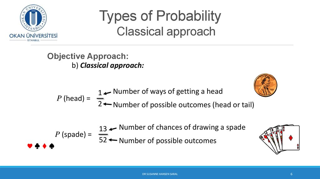
6. Types of Probability Classical approach

Objective Approach:
b) Classical approach:
1
P (head) =
2
♥♣♦♠
13
P (spade) =
52
Number of ways of getting a head
Number of possible outcomes (head or tail)
Number of chances of drawing a spade
Number of possible outcomes
DR SUSANNE HANSEN SARAL
6

7. Subjective approach to assign probabilities

We use the subjective approach :
No possibility to use the classical approach nor the relative frequency
approach.
No historic data available
New situation that nobody has been in so far
The probability will differ between two people, because it is subjective.
DR SUSANNE HANSEN SARAL
7

8. Types of Probability

Subjective Approach:
Based on the experience and judgment of the person making the
estimate:
◦ Opinion polls (broad public)
◦ Judgement of experts (professional judgement)
◦ Personal judgement
DR SUSANNE HANSEN SARAL
8

9. Interpreting probability

No matter what method is used to assign probabilities, we interpret the probability,
using the relative frequency approach for an infinite number of experiments.
The probability is only an estimate, because the relative frequency approach defines
probability as the “long-run” relative frequency.
The larger the number of observations the better the estimate will become.
Ex.: Tossing a coin, birth of a baby, etc.
Head and tail will only occur 50 % in the long run
Girl and boy will only occur 50 % in the long run
DR SUSANNE HANSEN SARAL
9

10. Probability rules continued Rule 1 and 2

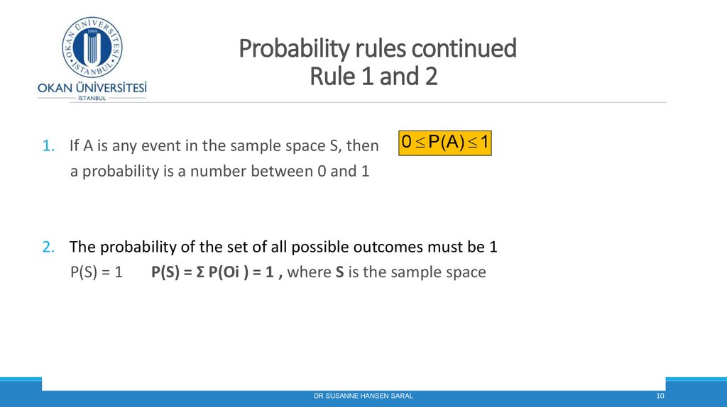
1. If A is any event in the sample space S, then
a probability is a number between 0 and 1
0 P(A) 1
2. The probability of the set of all possible outcomes must be 1
P(S) = 1
P(S) = Σ P(Oi ) = 1 , where S is the sample space
DR SUSANNE HANSEN SARAL
10

11. Objective probability assessment – The Relative Frequency Approach

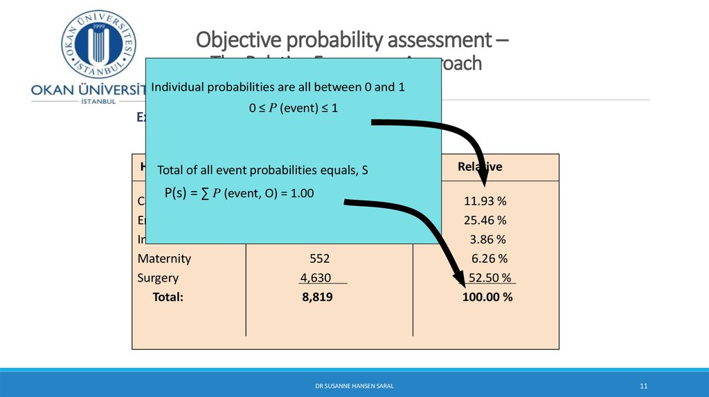
Individual probabilities are all between 0 and 1
0 ≤ P (event) ≤ 1
Example: Hospital Patients by Unit per semester
Hospital
Unit
Number of equals,
PatientsS
Total of
all event probabilities
Frequency
P(s) = ∑ P (event, O) = 1.00
Cardiac Care
1,052
Emergency
2,245
Intensive Care
340
Maternity
552
Surgery
4,630
Total:
8,819
DR SUSANNE HANSEN SARAL
Relative
11.93 %
25.46 %
3.86 %
6.26 %
52.50 %
100.00 %
11

12. Probability rules. Rule 3 Complement rule

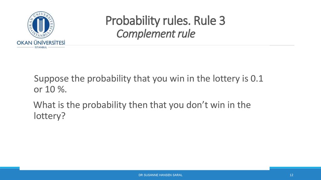
Suppose the probability that you win in the lottery is 0.1
or 10 %.
What is the probability then that you don’t win in the
lottery?
DR SUSANNE HANSEN SARAL
12

13. Probability rules. Rule 3 Complement rule

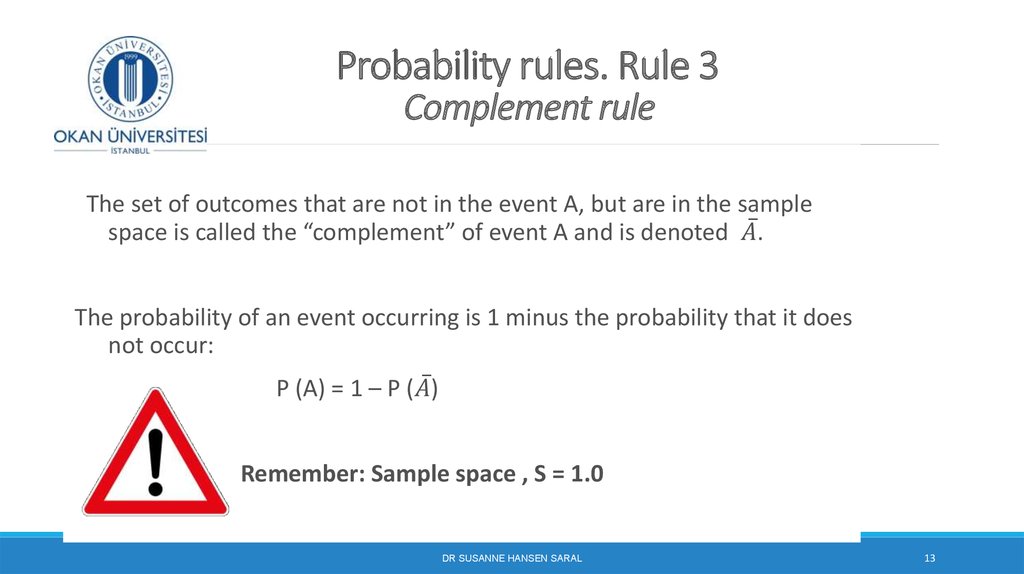
The set of outcomes that are not in the event A, but are in the sample
space is called the “complement” of event A and is denoted