Klasyczna procedura dla szeregów bez sezonowości

Summary of the Behaviour of autocorrelation and partial autocorrelation functions

1.35M

Category: $mathematics$ mathematics

Modele Boxa-Jenkinsa

1. Modele Boxa-Jenkinsa (ARIMA)

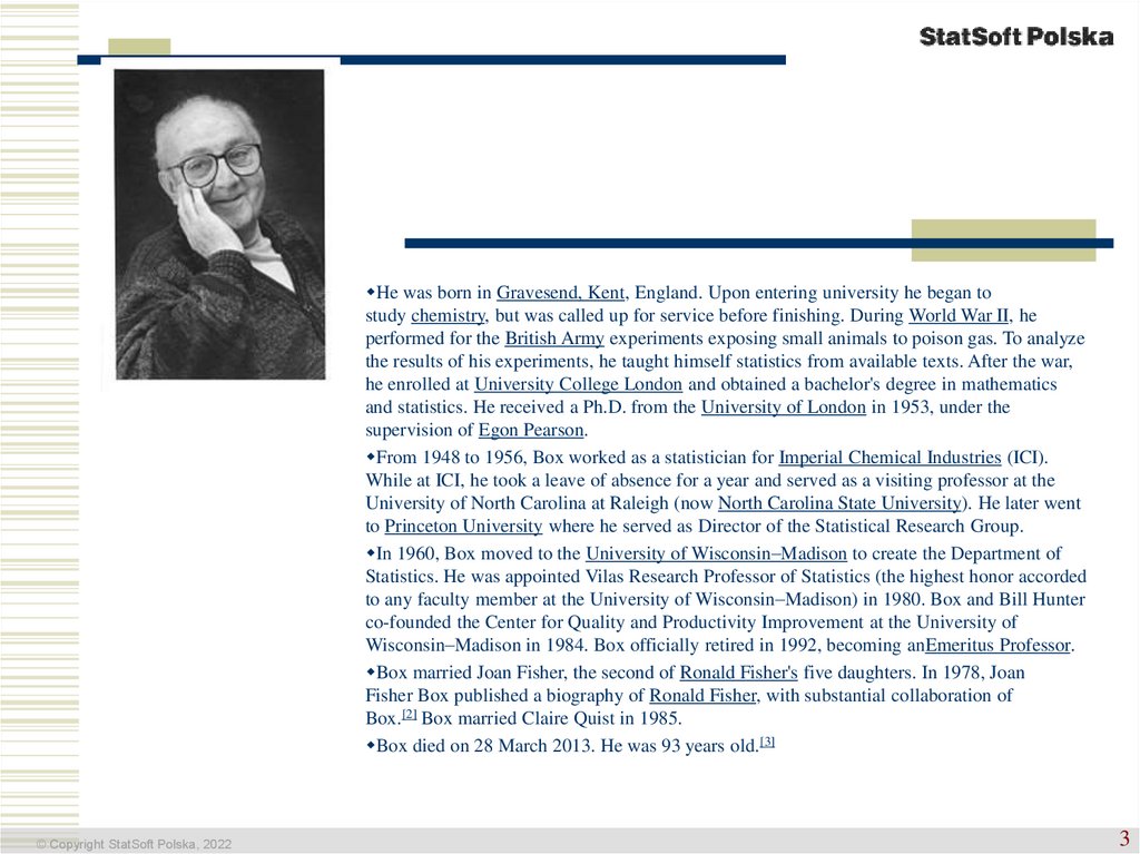
He was born in Gravesend, Kent, England. Upon entering university he began to
study chemistry, but was called up for service before finishing. During World War II, he
performed for the British Army experiments exposing small animals to poison gas. To analyze
the results of his experiments, he taught himself statistics from available texts. After the war,
he enrolled at University College London and obtained a bachelor's degree in mathematics
and statistics. He received a Ph.D. from the University of London in 1953, under the
supervision of Egon Pearson.
From 1948 to 1956, Box worked as a statistician for Imperial Chemical Industries (ICI).
While at ICI, he took a leave of absence for a year and served as a visiting professor at the
University of North Carolina at Raleigh (now North Carolina State University). He later went
to Princeton University where he served as Director of the Statistical Research Group.
In 1960, Box moved to the University of Wisconsin–Madison to create the Department of
Statistics. He was appointed Vilas Research Professor of Statistics (the highest honor accorded
to any faculty member at the University of Wisconsin–Madison) in 1980. Box and Bill Hunter
co-founded the Center for Quality and Productivity Improvement at the University of
Wisconsin–Madison in 1984. Box officially retired in 1992, becoming anEmeritus Professor.
Box married Joan Fisher, the second of Ronald Fisher's five daughters. In 1978, Joan
Fisher Box published a biography of Ronald Fisher, with substantial collaboration of
Box.[2] Box married Claire Quist in 1985.
Box died on 28 March 2013. He was 93 years old.[3]
© Copyright StatSoft Polska, 2022
3

4.

Gwilym Meirion Jenkins (12 August 1932 – 10 July 1982) was
a Welsh statistician and systems engineer, born in Gowerton
(Welsh: Tregŵyr), Swansea, Wales.[1] He is most notable for his pioneering work
with George Box on autoregressive moving average models, also called BoxJenkins models, in time-series analysis. He earned a first class honours degree in
Mathematics in 1953 followed by a Ph.D. at University College London in 1956. After
graduating, he married Margaret Bellingham and together they raised three children. His
first job after university was junior fellow at theRoyal Aircraft Establishment. He followed
this by a series of visiting lecturer and professor positions at Imperial College
London, Stanford University, Princeton University, and the University of Wisconsin–
Madison, before settling in as a professor of Systems Engineering at Lancaster University in
1965. His initial work concerned discrete time domain models for Chemical
Engineering applications.
While at Lancaster, he founded and became managing director of ISCOL (International
Systems Corporation of Lancaster). He remained in academia until 1974, when he left to
start his own consulting company.
He served on the Research Section Committee and Council of the Royal Statistical
Society in the 1960s, founded the Journal of Systems Engineering in 1969, and briefly
carried out public duties with the Royal Treasury in the mid-1970s. He was elected to
theInstitute of Mathematical Statistics and the Institute of Statisticians.
He was a jazz and blues enthusiast and an accomplished pianist.
He succumbed to Hodgkin's lymphoma in 1982.
© Copyright StatSoft Polska, 2022
4

5.

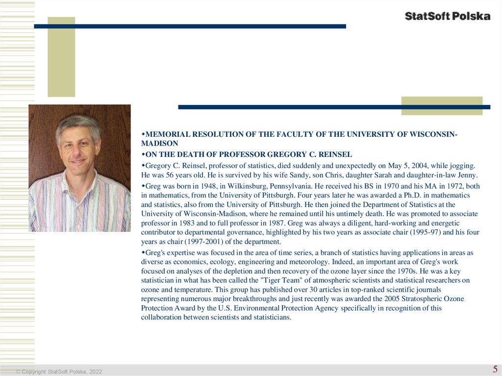
MEMORIAL RESOLUTION OF THE FACULTY OF THE UNIVERSITY OF WISCONSINMADISON
ON THE DEATH OF PROFESSOR GREGORY C. REINSEL
Gregory C. Reinsel, professor of statistics, died suddenly and unexpectedly on May 5, 2004, while jogging.
He was 56 years old. He is survived by his wife Sandy, son Chris, daughter Sarah and daughter-in-law Jenny.
Greg was born in 1948, in Wilkinsburg, Pennsylvania. He received his BS in 1970 and his MA in 1972, both
in mathematics, from the University of Pittsburgh. Four years later he was awarded a Ph.D. in mathematics
and statistics, also from the University of Pittsburgh. He then joined the Department of Statistics at the
University of Wisconsin-Madison, where he remained until his untimely death. He was promoted to associate
professor in 1983 and to full professor in 1987. Greg was always a diligent, hard-working and energetic
contributor to departmental governance, highlighted by his two years as associate chair (1995-97) and his four
years as chair (1997-2001) of the department.
Greg's expertise was focused in the area of time series, a branch of statistics having applications in areas as
diverse as economics, ecology, engineering and meteorology. Indeed, an important area of Greg's work
focused on analyses of the depletion and then recovery of the ozone layer since the 1970s. He was a key
statistician in what has been called the "Tiger Team" of atmospheric scientists and statistical researchers on
ozone and temperature. This group has published over 30 articles in top-ranked scientific journals
representing numerous major breakthroughs and just recently was awarded the 2005 Stratospheric Ozone
Protection Award by the U.S. Environmental Protection Agency specifically in recognition of this
collaboration between scientists and statisticians.
© Copyright StatSoft Polska, 2022
5

6. Modele Boxa-Jenkinsa (ARIMA)

Metodologia Boxa-Jenkinsa to zbiór procedur identyfikacji i
szacowania modeli szeregów czasowych w klasie zintegrowanych
modeli autoregresji średniej ruchomej (ARIMA).
Modele ARIMA to modele regresyjne wykorzystujące opóźnioną
zmienną zależną oraz składniki losowe jako zmienne objaśniające
Postać modeli ARIMA zależy od autokorelacji obserwowanych w
szeregu
Metoda może być stosowana do danych bez składowych
okresowych, jak i do szeregów zawierających takie wahania
© Copyright StatSoft Polska, 2022
6

7. Modele Boxa-Jenkinsa (ARIMA)

Trzy podstawowe modele ARIMA dla
stacjonarnych szeregów czasowych yt :
(1) Model autoregresji rzędu p (AR(p))
yt 1 yt 1 2 yt 2 p yt p t ,
gdzie yt zależy od p swoich poprzednich wartości
(2) Model średniej ruchomej rzędu q (MA(q))
yt t 1 t 1 2 t 2 q t q ,
gdzie yt zależy od q poprzednich składników
losowych
© Copyright StatSoft Polska, 2022
7

8. Modele Boxa-Jenkinsa (ARIMA)

(3) Model autoregresji średniej ruchomej rzędu p i
q (ARMA(p,q))
yt 1 yt 1 2 yt 2 p yt p
t 1 t 1 2 t 2 q t q ,
gdzie yt zależy od p swoich poprzednich wartości
oraz q poprzednich składników losowych
© Copyright StatSoft Polska, 2022
8

9. Modele Boxa-Jenkinsa

W modelu ARIMA, że składnik losowy
t jest “białym szumem”; to znaczy jest ciągirm
niezależnych zmiennych losowych o jednakowym
rozkładzie z wartością przeciętną 0 i stałą wariancją
2
Zapisujemy to:
t ~ i.i.d.(0, )
© Copyright StatSoft Polska, 2022
9

10. Klasyczna procedura dla szeregów bez sezonowości

1) Testowanie stacjonarności i różnicowanie
(poszukiwanie trendu i jego eliminacja)
2) Identyfikacja modelu (ustalenie p i q)
3) Estymacja parametrów modelu
4) Weryfikacja modelu
5) Prognozowanie
© Copyright StatSoft Polska, 2022
10

11. Przykład białego szumu

12. Przykład szeregu niestacjonarnego

13. Najczęstsze rodzaje niestacjonarności

14. Model z uwzględnieniem wahań okresowych

ARIMA (p, d, q)(Ps, Ds, Qs)
Pierwszy nawias to część niesezonowa
Drugi nawias to część sezonowa
S – długość cyklu wahań sezonowych (4, 7,
12, itp.)
My mamy zadać wartości zawarte w
nawiasach. Na tym polega identyfikacja
modelu.
© Copyright StatSoft Polska, 2022
14

15. Praktyczne budowanie modelu (S)ARIMA

16. Identyfikacja modelu

17. ARIMA (p, d, q)(Ps, Ds, Qs)

18. ARIMA (p, d, q)(Ps, Ds, Qs)

S – długość podstawowego cyklu sezonowego
(okresowego)
Dla danych kwartalnych 4; dla danych
miesięcznych 12; dla danych dziennych 7, dla
danych godzinowych 24
Jak jest kilka cykli to te wartości trzeba mnożyć,
np. 7 dni x 24 godziny = 168
Rysunek
Funkcja autokorelacji
© Copyright StatSoft Polska, 2022
18

19. ARIMA (p, d, q)(Ps, Ds, Qs)

20. ARIMA (p, d, q)(Ps, Ds, Qs)

Trzeba odgadnąć ile wynoszą p i q
Box i Jenkins zalecali oglądanie funkcji
autokorelacji i funkcji autokorelacji
cząstkowej i na tej podstawie odgadywanie p
i q. Ale to działało tylko do p, q 2
A.S.: podstawić p=q=1 i ewentualnie
zwiększać weryfikując poprawność modelu
© Copyright StatSoft Polska, 2022
20

21. Summary of the Behaviour of autocorrelation and partial autocorrelation functions

Behaviour of autocorrelation and partial autocorrelation functions
Model
Autoregressive of order p
yt 1 yt 1 2 yt 2
p yt p t
Moving Average of order q
yt t 1 t 1 2 t 2
q t q
Mixed Autoregressive-Moving Average of order (p,q)
yt 1 yt 1 2 yt 2 p yt p
t 1 t 1 2 t 2
© Copyright StatSoft Polska, 2022
AC
PAC
Dies down Cuts off
after lag p
Cuts off
Dies down
after lag q
Dies down Dies down
q t q
21

22. Summary of the Behaviour of autocorrelation and partial autocorrelation functions

Behaviour of AC and PAC for specific non-seasonal models
Model
AC
PAC
First-order autoregressive
yt 1 yt 1 t
Dies down in a damped exponential
fashion; specifically:
Cuts off
after lag
1
Second-order autoregressive
yt 1 yt 1 2 yt 2 t
Dies down according to a mixture of
damped exponentials and/or damped
sine waves; specifically:
1 1 ,
1 2
Cuts off
after lag
2
k 1k for k 1
12
2 2
,
1 2
k 1 k 1 2 k 2 for k 3
© Copyright StatSoft Polska, 2022
22

23. Summary of the Behaviour of autocorrelation and partial autocorrelation functions

Behaviour of AC and PAC for specific non-seasonal models
Model
First-order moving average
yt t 1 t 1
AC
PAC
Cuts off after lag 1; specifically: Dies down in a fashion
1
dominated by damped
1
,
2
1 1
exponential decay
k 0 for k 2
Second-order moving average
Cuts off after lag 2; specifically: Dies down according
1 (1 2 )
to a mixture of
yt t 1 t 1 2 t 2
1
,
2
2
damped exponentials
1 1 2
and/or damped sine
2
2
,
waves
2
2
1 1 2
k 0 for k 2.
© Copyright StatSoft Polska, 2022
23

24. Summary of the Behaviour of autocorrelation and partial autocorrelation functions

Behaviour of AC and PAC for specific non-seasonal models
Model
Mixed autoregressivemovingaverage of order (1,1)
yt 1 yt 1 t 1 t 1
AC
Dies down in a damped
exponential fashion;
specifically:
1
(1 1 1 )( 1 1 )
,
2
1 1 2 1 1
PAC
Dies down in a
fashion dominated
by damped
exponential decay
k 1 k 1 for k 2
© Copyright StatSoft Polska, 2022
24

25. Estymacja parametrów

26. Weryfikacja modelu

27. Weryfikacja modelu

Model powinien dać się oszacować
Istotność parametrów strukturalnych
Regresja krokowa (zmienianie p, q, Ps, Qs)
Autokorelacja reszt (powinno jej nie być)
Rozkład reszt
© Copyright StatSoft Polska, 2022
27

28. Prognozowanie

English Русский Rules