Dense Linear Algebra: History and Structure, Parallel Matrix Multiplication

1. CS 267 Dense Linear Algebra: History and Structure, Parallel Matrix Multiplication

James Demmel
www.cs.berkeley.edu/~demmel/cs267_Spr11
02/22/2011
CS267 Lecture 11
1

2. Outline

History and motivation
Structure of the Dense Linear Algebra motif
Parallel Matrix-matrix multiplication
Parallel Gaussian Elimination (next time)
02/22/2011
CS267 Lecture 11
2

3. Outline

History and motivation
Structure of the Dense Linear Algebra motif
Parallel Matrix-matrix multiplication
Parallel Gaussian Elimination (next time)
02/22/2011
CS267 Lecture 11
3

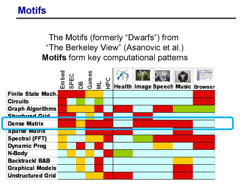
4. Motifs

The Motifs (formerly “Dwarfs”) from
“The Berkeley View” (Asanovic et al.)
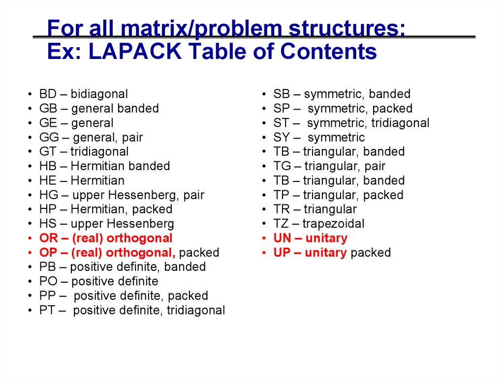
Motifs form key computational patterns
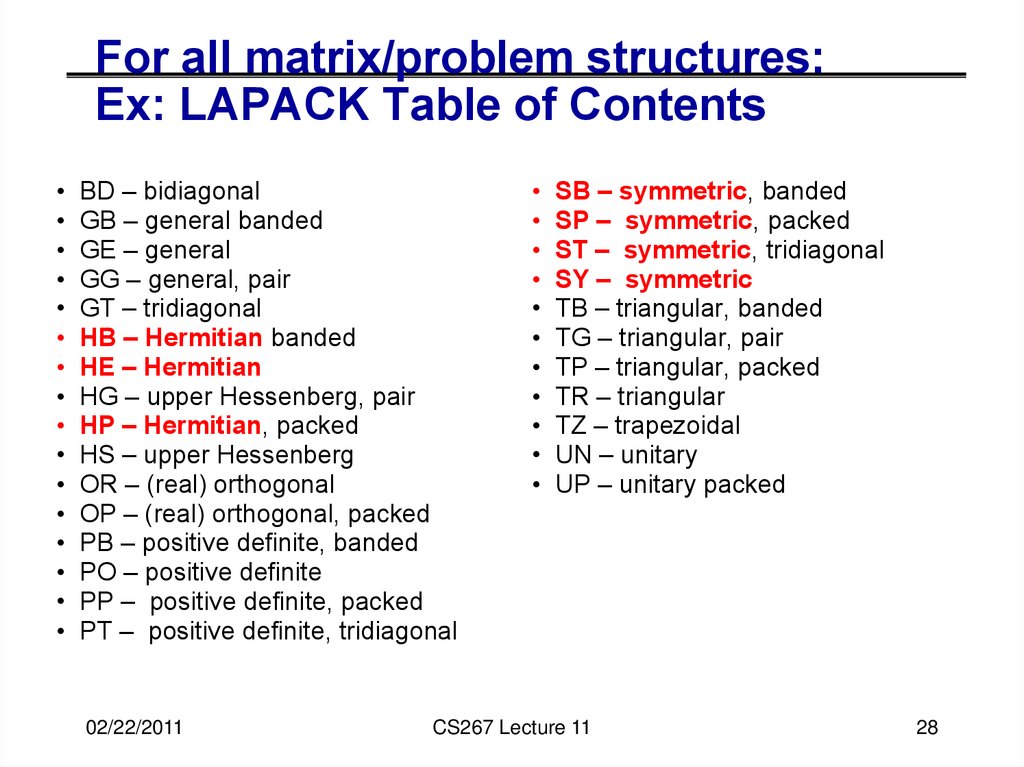
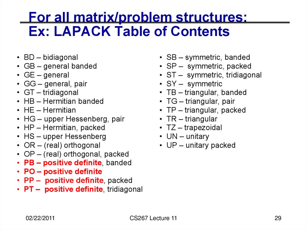
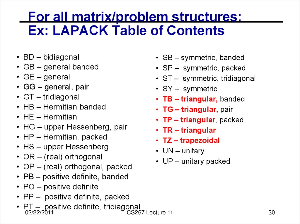
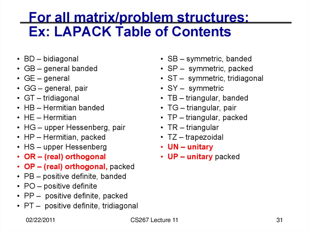
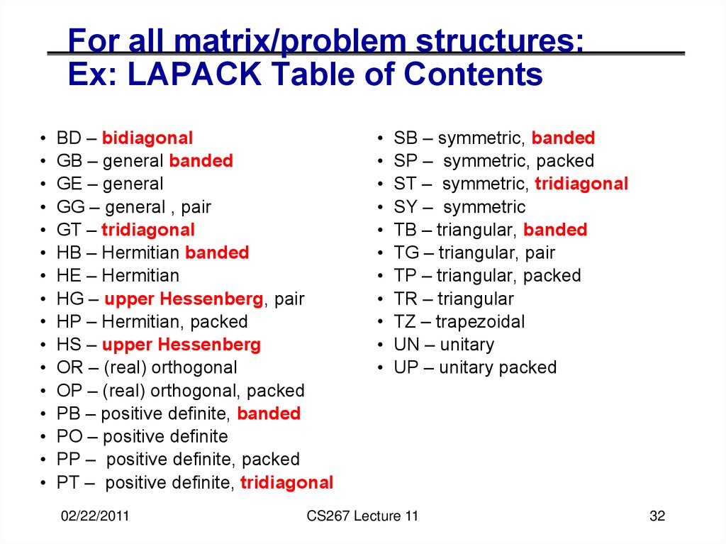
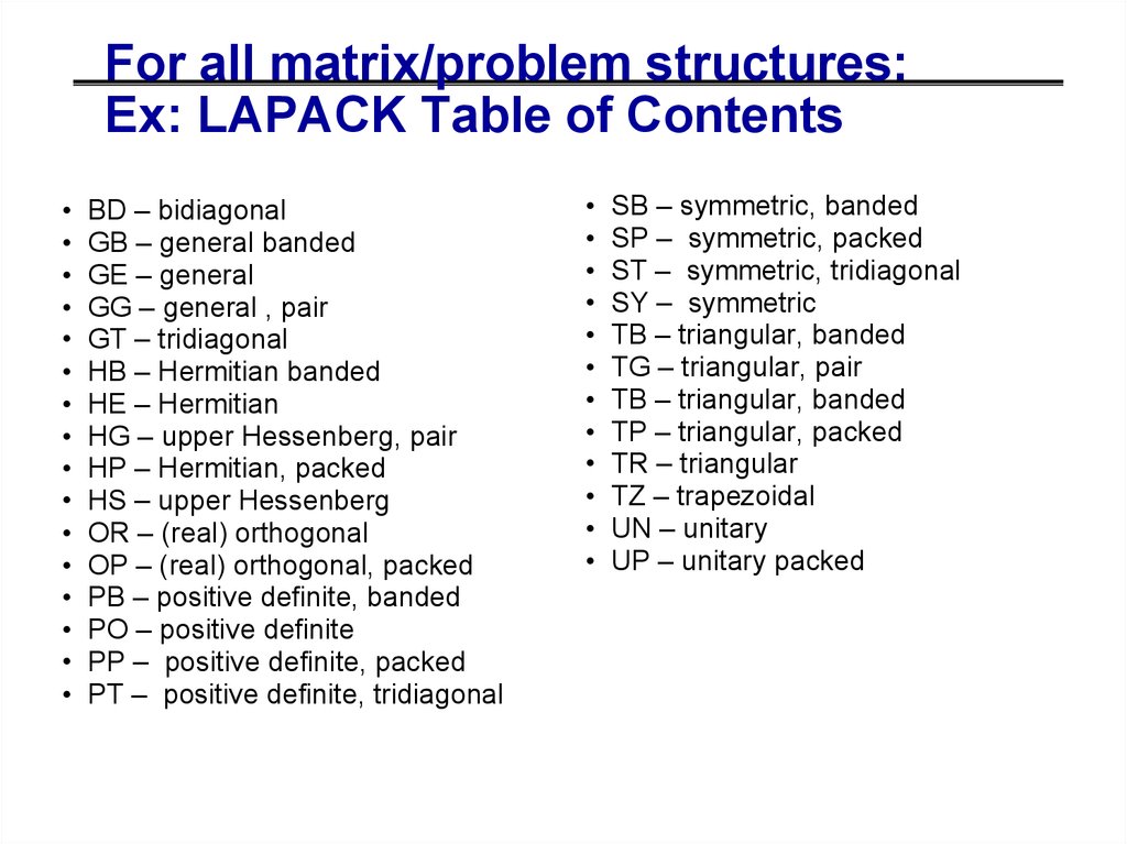
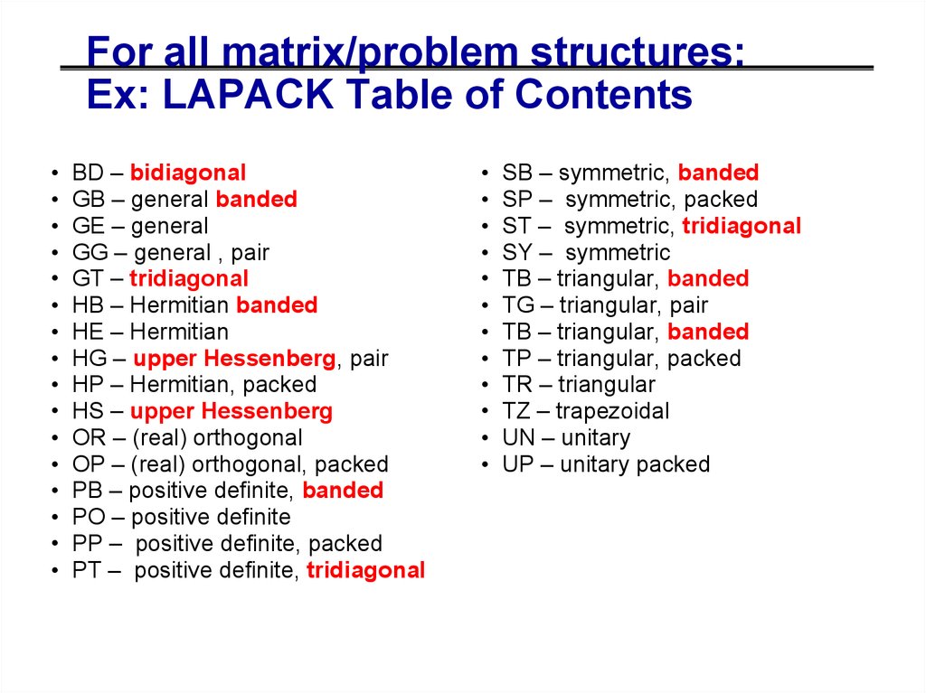
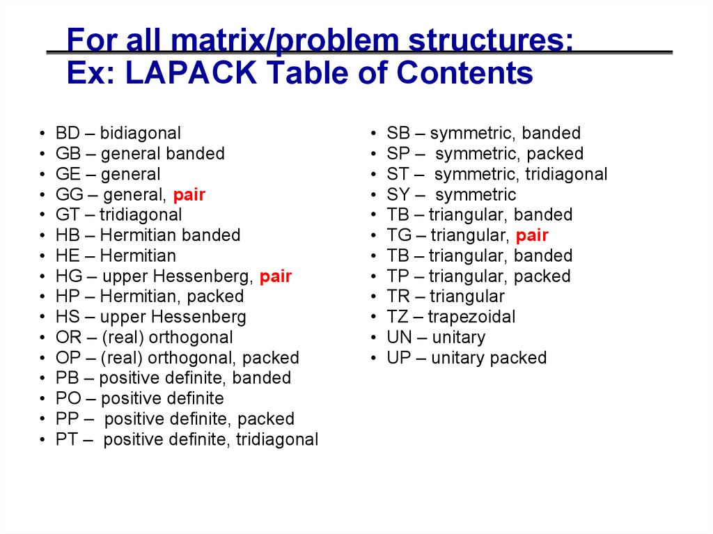
4

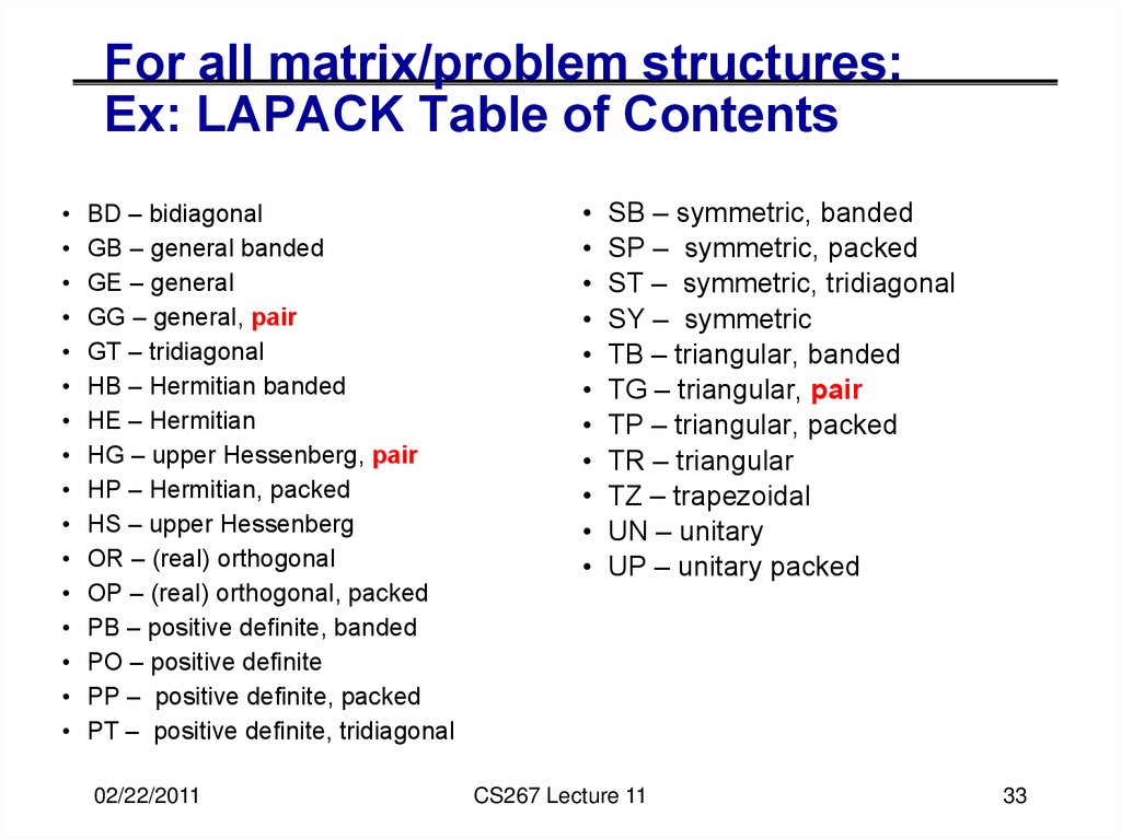
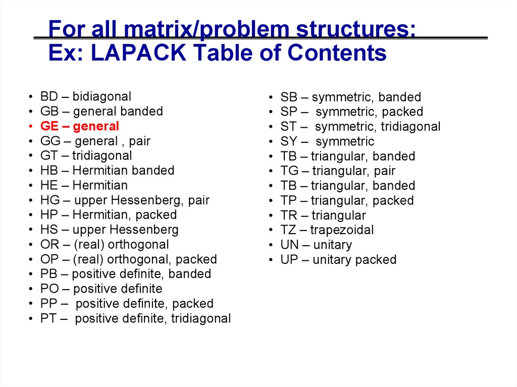
5. What is dense linear algebra?

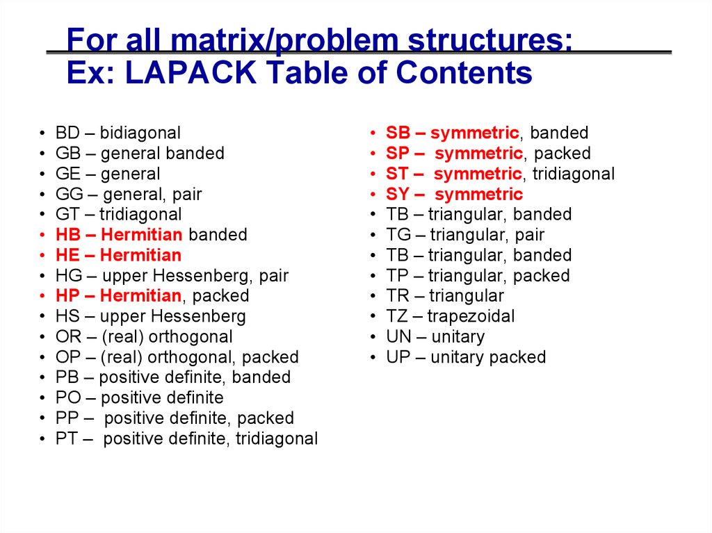
• Not just matmul!
• Linear Systems: Ax=b
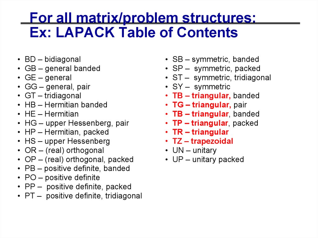
• Least Squares: choose x to minimize ||Ax-b||2
• Overdetermined or underdetermined
• Unconstrained, constrained, weighted
• Eigenvalues and vectors of Symmetric Matrices
Standard (Ax = λx), Generalized (Ax=λBx)
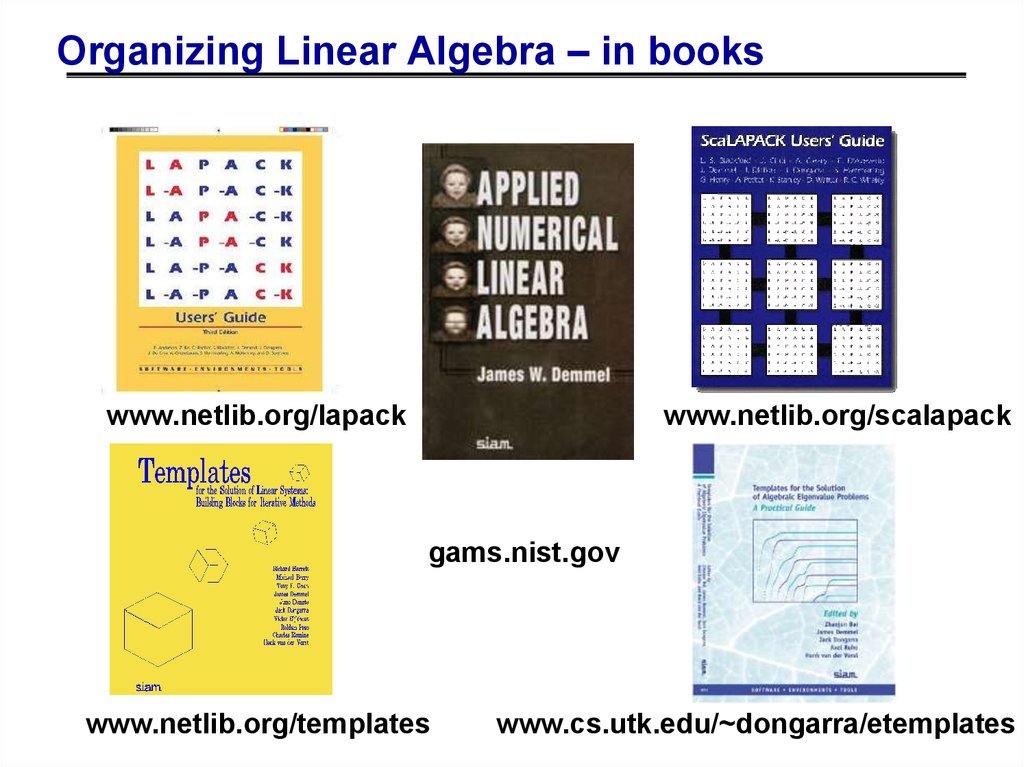
• Eigenvalues and vectors of Unsymmetric matrices
Eigenvalues, Schur form, eigenvectors, invariant subspaces
Standard, Generalized
• Singular Values and vectors (SVD)
• Standard, Generalized
• Different matrix structures
• Real, complex; Symmetric, Hermitian, positive definite; dense, triangular, banded …
• Level of detail
• Simple Driver
• Expert Drivers with error bounds, extra-precision, other options
• Lower level routines (“apply certain kind of orthogonal transformation”, matmul…)
02/22/2011
CS267 Lecture 11
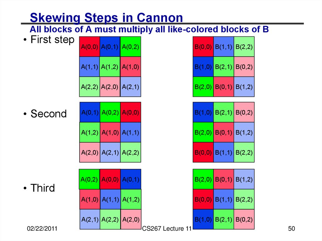
5

6. A brief history of (Dense) Linear Algebra software (1/7)

• In the beginning was the do-loop…
• Libraries like EISPACK (for eigenvalue problems)
• Then the BLAS (1) were invented (1973-1977)
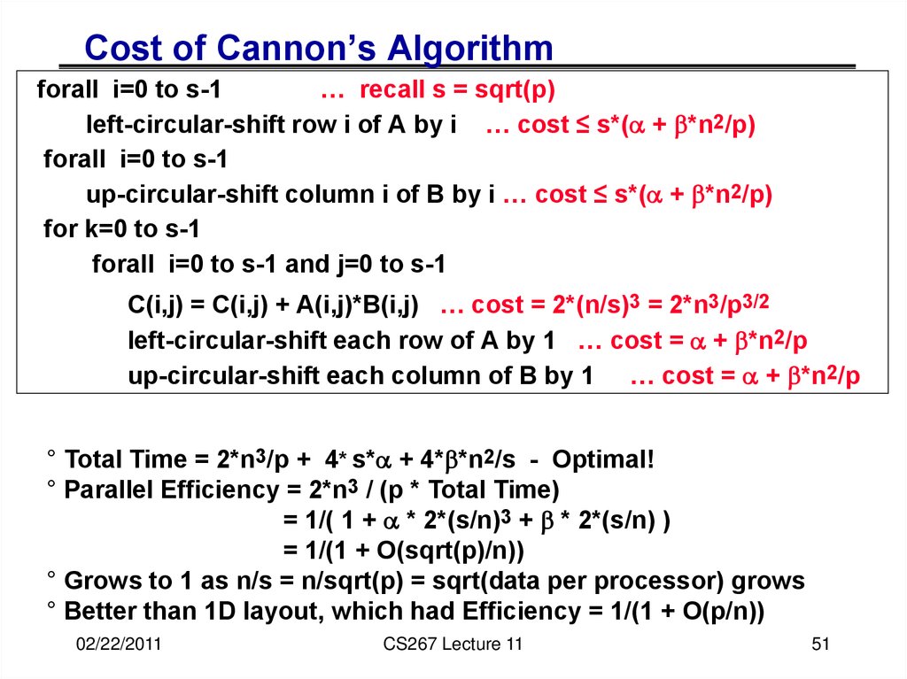
• Standard library of 15 operations (mostly) on vectors
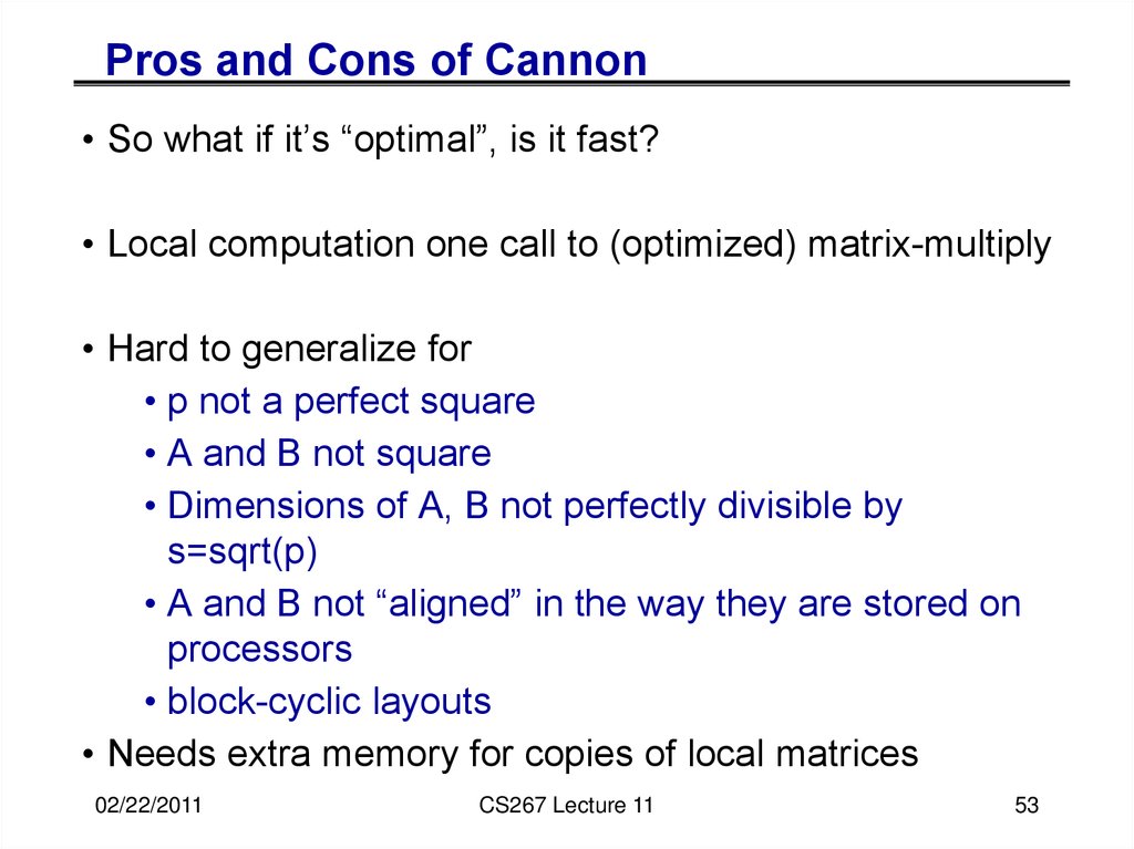
• “AXPY” ( y = α·x + y ), dot product, scale (x = α·x ), etc
• Up to 4 versions of each (S/D/C/Z), 46 routines, 3300 LOC
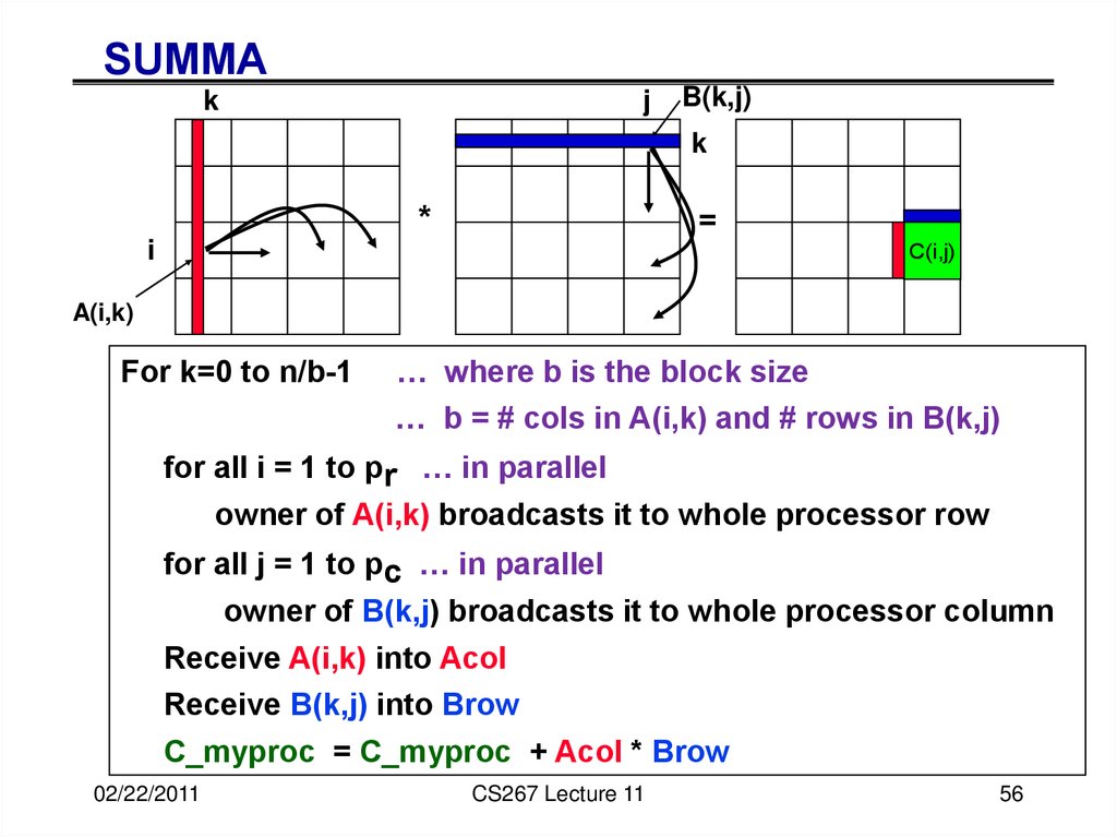
• Goals
• Common “pattern” to ease programming, readability, selfdocumentation
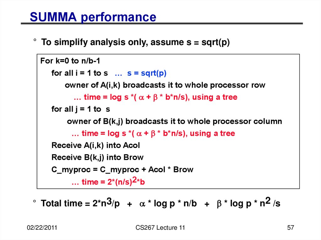
• Robustness, via careful coding (avoiding over/underflow)
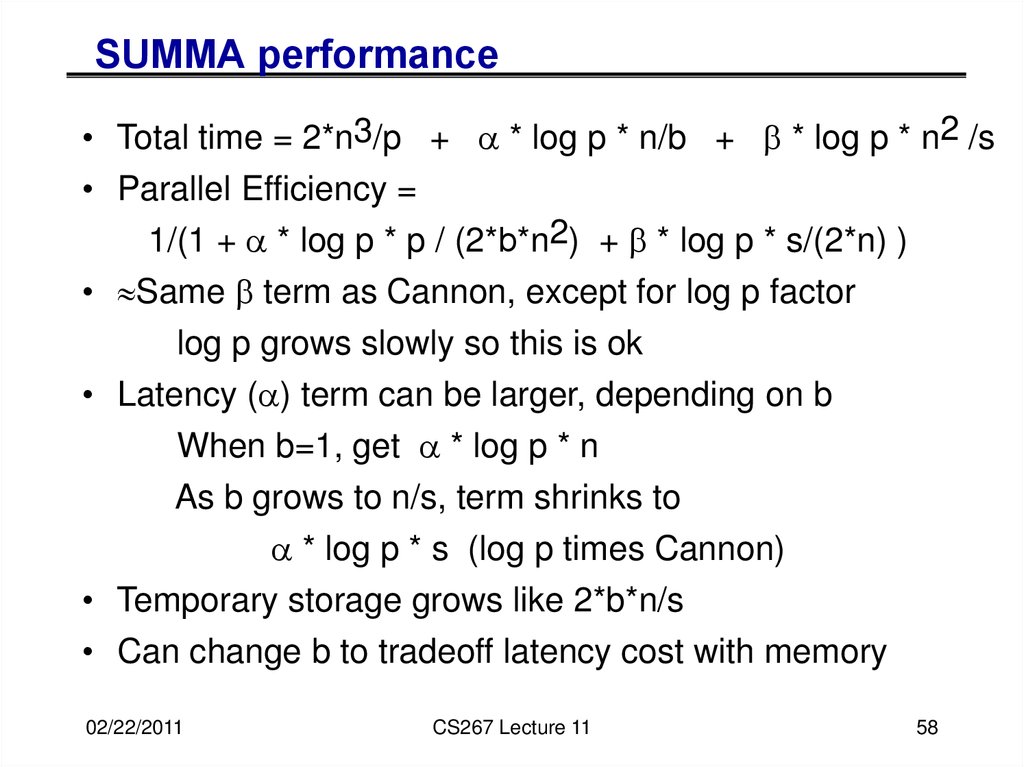
• Portability + Efficiency via machine specific implementations
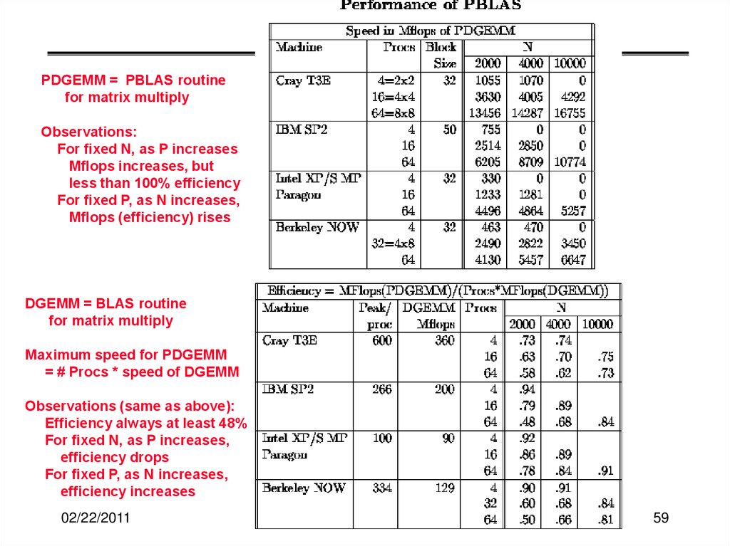
• Why BLAS 1 ? They do O(n1) ops on O(n1) data
• Used in libraries like LINPACK (for linear systems)
• Source of the name “LINPACK Benchmark” (not the code!)
02/22/2011
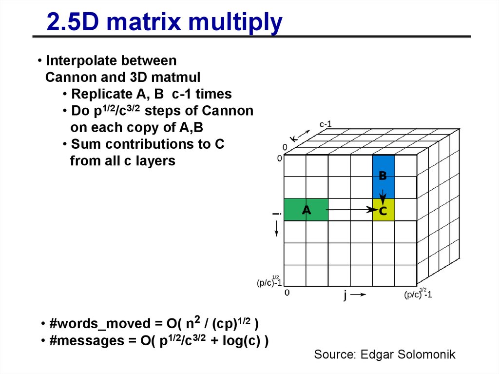
CS267 Lecture 11
6

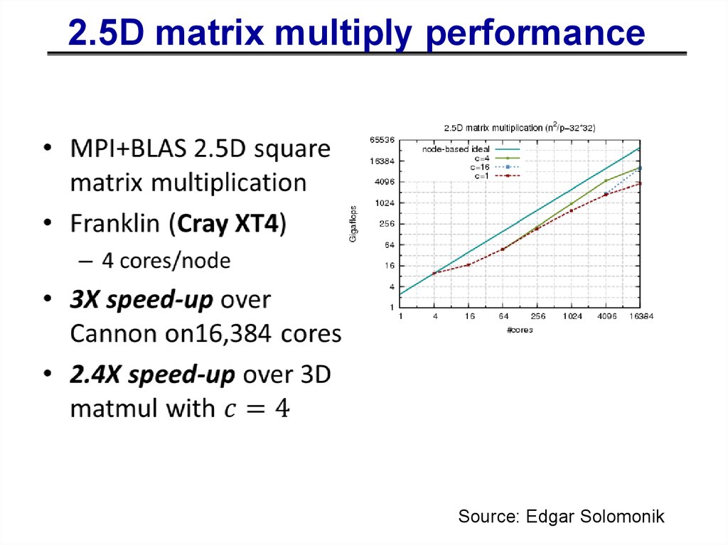
7.

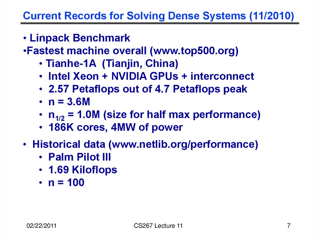
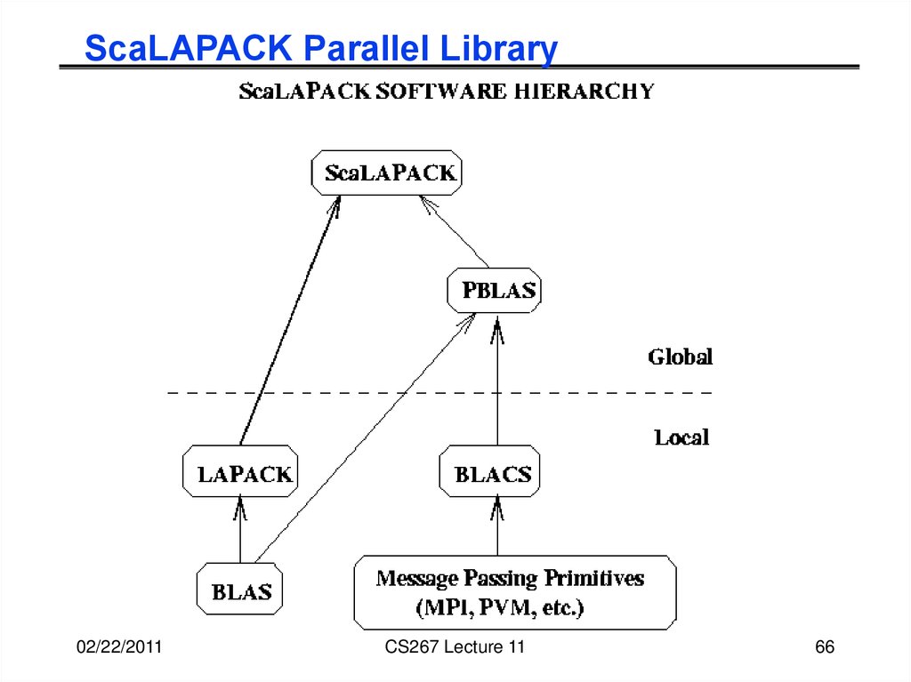
Current Records for Solving Dense Systems (11/2010)
• Linpack Benchmark
•Fastest machine overall (www.top500.org)
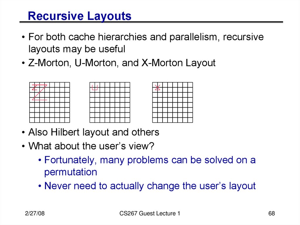
• Tianhe-1A (Tianjin, China)
• Intel Xeon + NVIDIA GPUs + interconnect
• 2.57 Petaflops out of 4.7 Petaflops peak
• n = 3.6M
• n1/2 = 1.0M (size for half max performance)
• 186K cores, 4MW of power
• Historical data (www.netlib.org/performance)
• Palm Pilot III
• 1.69 Kiloflops
• n = 100
02/22/2011
CS267 Lecture 11
7

8. A brief history of (Dense) Linear Algebra software (2/7)

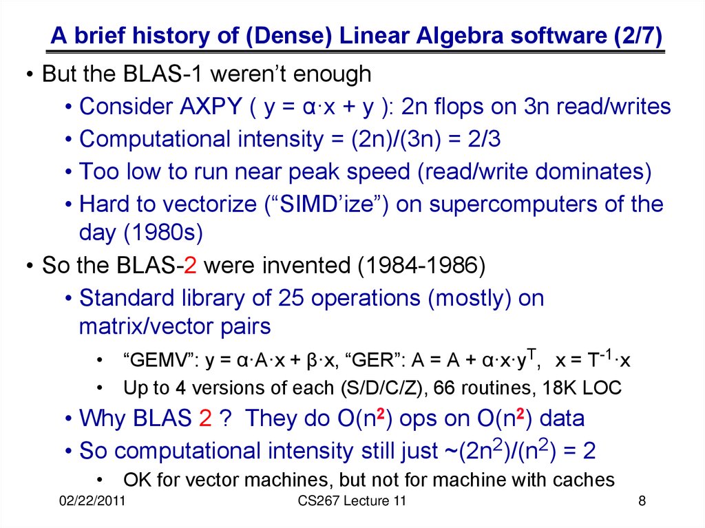
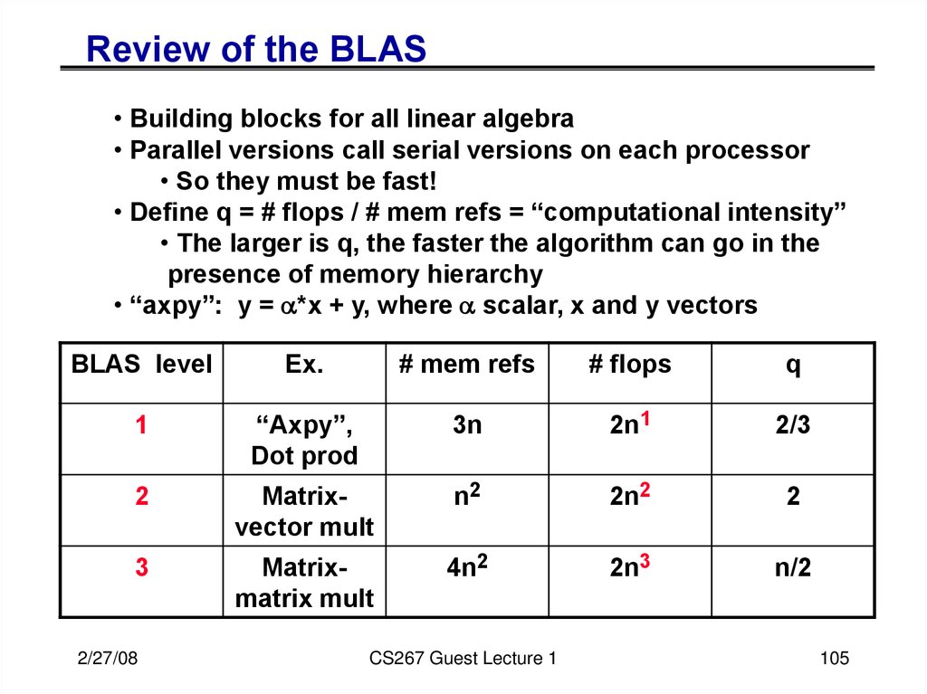
• But the BLAS-1 weren’t enough
• Consider AXPY ( y = α·x + y ): 2n flops on 3n read/writes
• Computational intensity = (2n)/(3n) = 2/3
• Too low to run near peak speed (read/write dominates)
• Hard to vectorize (“SIMD’ize”) on supercomputers of the
day (1980s)
• So the BLAS-2 were invented (1984-1986)
• Standard library of 25 operations (mostly) on
matrix/vector pairs
• “GEMV”: y = α·A·x + β·x, “GER”: A = A + α·x·yT, x = T-1·x
• Up to 4 versions of each (S/D/C/Z), 66 routines, 18K LOC
• Why BLAS 2 ? They do O(n2) ops on O(n2) data
• So computational intensity still just ~(2n2)/(n2) = 2
• OK for vector machines, but not for machine with caches
02/22/2011
CS267 Lecture 11
8

9. A brief history of (Dense) Linear Algebra software (3/7)

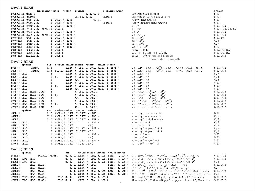
• The next step: BLAS-3 (1987-1988)
• Standard library of 9 operations (mostly) on matrix/matrix pairs
• “GEMM”: C = α·A·B + β·C, C = α·A·AT + β·C, B = T-1·B
• Up to 4 versions of each (S/D/C/Z), 30 routines, 10K LOC
• Why BLAS 3 ? They do O(n3) ops on O(n2) data
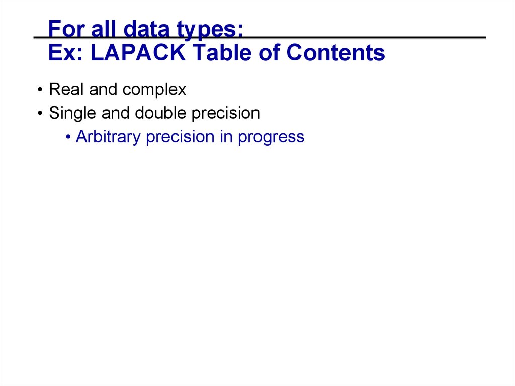
• So computational intensity (2n3)/(4n2) = n/2 – big at last!
• Good for machines with caches, other mem. hierarchy levels
• How much BLAS1/2/3 code so far (all at www.netlib.org/blas)
• Source: 142 routines, 31K LOC,
Testing: 28K LOC
• Reference (unoptimized) implementation only
• Ex: 3 nested loops for GEMM
• Lots more optimized code (eg Homework 1)
• Motivates “automatic tuning” of the BLAS
• Part of standard math libraries (eg AMD AMCL, Intel MKL)
02/22/2011
CS267 Lecture 11
9

10.

02/25/2009
CS267 Lecture 8
10

11. A brief history of (Dense) Linear Algebra software (4/7)

• LAPACK – “Linear Algebra PACKage” - uses BLAS-3 (1989 – now)
• Ex: Obvious way to express Gaussian Elimination (GE) is adding
multiples of one row to other rows – BLAS-1
How do we reorganize GE to use BLAS-3 ? (details later)
• Contents of LAPACK (summary)
Algorithms we can turn into (nearly) 100% BLAS 3
– Linear Systems: solve Ax=b for x
– Least Squares: choose x to minimize ||Ax-b||2
Algorithms that are only 50% BLAS 3
– Eigenproblems: Find l and x where Ax = l x
– Singular Value Decomposition (SVD)
Generalized problems (eg Ax = l Bx)
Error bounds for everything
Lots of variants depending on A’s structure (banded, A=AT, etc)
• How much code? (Release 3.3, Nov 2010) (www.netlib.org/lapack)
Source: 1586 routines, 500K LOC, Testing: 363K LOC
• Ongoing development (at UCB and elsewhere) (class projects!)
02/22/2011
CS267 Lecture 11
11

12. A brief history of (Dense) Linear Algebra software (5/7)

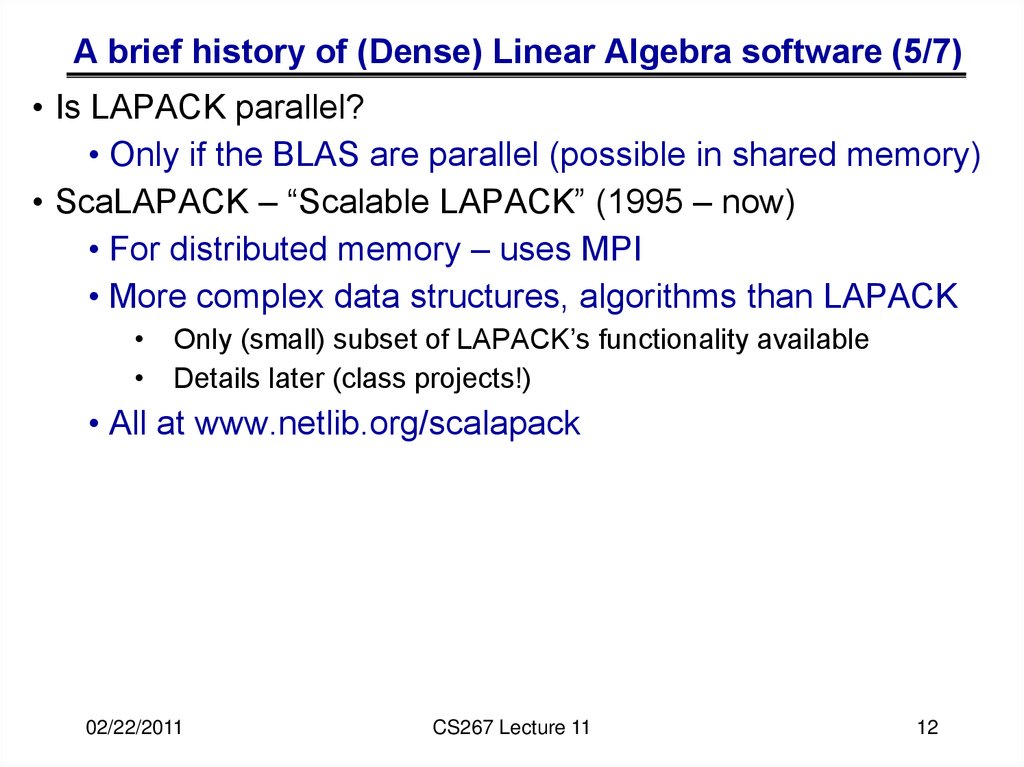
• Is LAPACK parallel?
• Only if the BLAS are parallel (possible in shared memory)
• ScaLAPACK – “Scalable LAPACK” (1995 – now)
• For distributed memory – uses MPI
• More complex data structures, algorithms than LAPACK
• Only (small) subset of LAPACK’s functionality available
• Details later (class projects!)
• All at www.netlib.org/scalapack
02/22/2011
CS267 Lecture 11
12

13. Success Stories for Sca/LAPACK (6/7)

• Widely used
• Adopted by Mathworks, Cray,
Fujitsu, HP, IBM, IMSL, Intel,
NAG, NEC, SGI, …
• 5.5M webhits/year @ Netlib
(incl. CLAPACK, LAPACK95)
• New Science discovered through the
solution of dense matrix systems
• Nature article on the flat
universe used ScaLAPACK
• Other articles in Physics
Review B that also use it
• 1998 Gordon Bell Prize
• www.nersc.gov/news/reports/
newNERSCresults050703.pdf
02/22/2011
Cosmic Microwave Background
Analysis, BOOMERanG
collaboration, MADCAP code (Apr.
27, 2000).
CS267 Lecture 11
ScaLAPACK
13

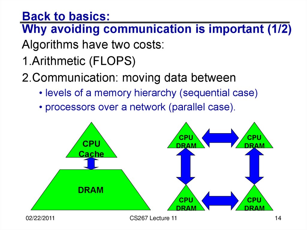
14. Back to basics: Why avoiding communication is important (1/2)

Algorithms have two costs:
1.Arithmetic (FLOPS)
2.Communication: moving data between
• levels of a memory hierarchy (sequential case)
• processors over a network (parallel case).
CPU
Cache
CPU
DRAM
CPU
DRAM
CPU
DRAM
CPU
DRAM
DRAM
02/22/2011
CS267 Lecture 11
14

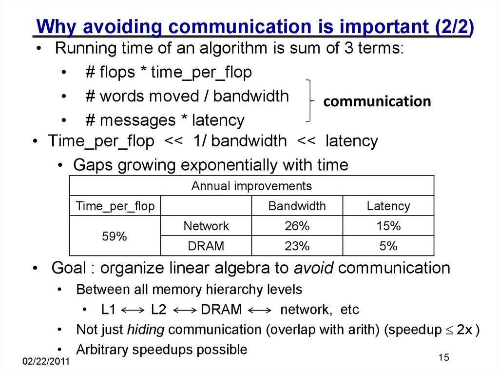
15. Why avoiding communication is important (2/2)

• Running time of an algorithm is sum of 3 terms:
• # flops * time_per_flop
• # words moved / bandwidth
communication
• # messages * latency
• Time_per_flop << 1/ bandwidth << latency
• Gaps growing exponentially with time
Annual improvements
Time_per_flop
59%
Bandwidth
Latency
Network
26%
15%
DRAM
23%
5%
• Goal : organize linear algebra to avoid communication
• Between all memory hierarchy levels
• L1
L2
DRAM
network, etc
• Not just hiding communication (overlap with arith) (speedup 2x )
• Arbitrary speedups possible
15
02/22/2011

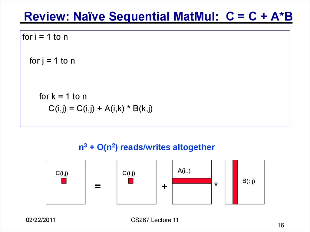
16. Review: Naïve Sequential MatMul: C = C + A*B

for i = 1 to n
{read row i of A into fast memory, n2 reads}
for j = 1 to n
{read C(i,j) into fast memory, n2 reads}
{read column j of B into fast memory, n3 reads}
for k = 1 to n
C(i,j) = C(i,j) + A(i,k) * B(k,j)
{write C(i,j) back to slow memory, n2 writes}
n3 + O(n2) reads/writes altogether
C(i,j)
=
02/22/2011
A(i,:)
C(i,j)
+
CS267 Lecture 11
*
B(:,j)
16

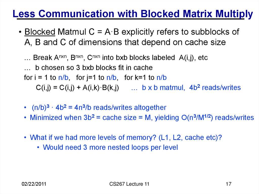
17. Less Communication with Blocked Matrix Multiply

• Blocked Matmul C = A·B explicitly refers to subblocks of
A, B and C of dimensions that depend on cache size
… Break Anxn, Bnxn, Cnxn into bxb blocks labeled A(i,j), etc
… b chosen so 3 bxb blocks fit in cache
for i = 1 to n/b, for j=1 to n/b, for k=1 to n/b
C(i,j) = C(i,j) + A(i,k)·B(k,j)
… b x b matmul, 4b2 reads/writes
• (n/b)3 · 4b2 = 4n3/b reads/writes altogether
• Minimized when 3b2 = cache size = M, yielding O(n3/M1/2) reads/writes
• What if we had more levels of memory? (L1, L2, cache etc)?
• Would need 3 more nested loops per level
02/22/2011
CS267 Lecture 11
17

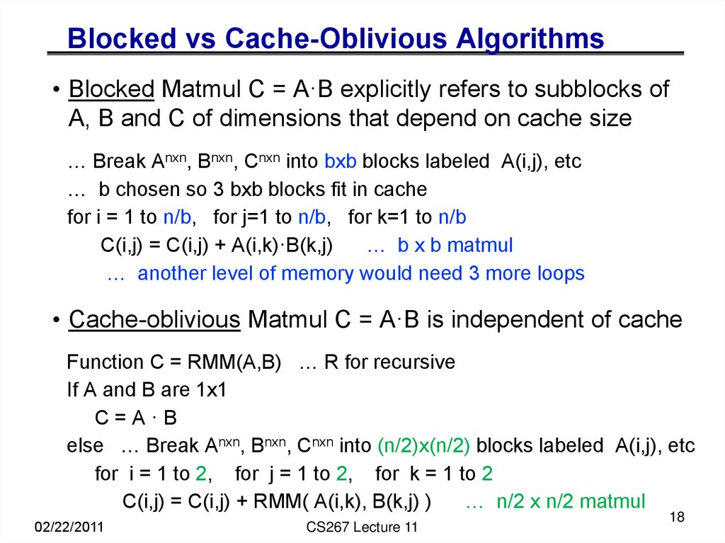
18. Blocked vs Cache-Oblivious Algorithms

• Blocked Matmul C = A·B explicitly refers to subblocks of
A, B and C of dimensions that depend on cache size
… Break Anxn, Bnxn, Cnxn into bxb blocks labeled A(i,j), etc
… b chosen so 3 bxb blocks fit in cache
for i = 1 to n/b, for j=1 to n/b, for k=1 to n/b
C(i,j) = C(i,j) + A(i,k)·B(k,j)
… b x b matmul
… another level of memory would need 3 more loops
• Cache-oblivious Matmul C = A·B is independent of cache
Function C = RMM(A,B) … R for recursive
If A and B are 1x1
C=A·B
else … Break Anxn, Bnxn, Cnxn into (n/2)x(n/2) blocks labeled A(i,j), etc
for i = 1 to 2, for j = 1 to 2, for k = 1 to 2
C(i,j) = C(i,j) + RMM( A(i,k), B(k,j) )
… n/2 x n/2 matmul
02/22/2011
CS267 Lecture 11
18

19. Communication Lower Bounds: Prior Work on Matmul

• Assume n3 algorithm (i.e. not Strassen-like)
• Sequential case, with fast memory of size M
• Lower bound on #words moved to/from slow memory =
(n3 / M1/2 ) [Hong, Kung, 81]
• Attained using blocked or cache-oblivious algorithms
• Parallel case on P processors:
• Let NNZ be total memory needed; assume load balanced
• Lower bound on #words moved
= (n3 /(p · NNZ1/2 ))
[Irony, Tiskin, Toledo, 04]
• If NNZ = 3n2/p (one copy of each matrix), then
lower bound = (n2 /p1/2 )
• Attained by Cannon’s algorithm
02/22/2011
CS267 Lecture 11
19

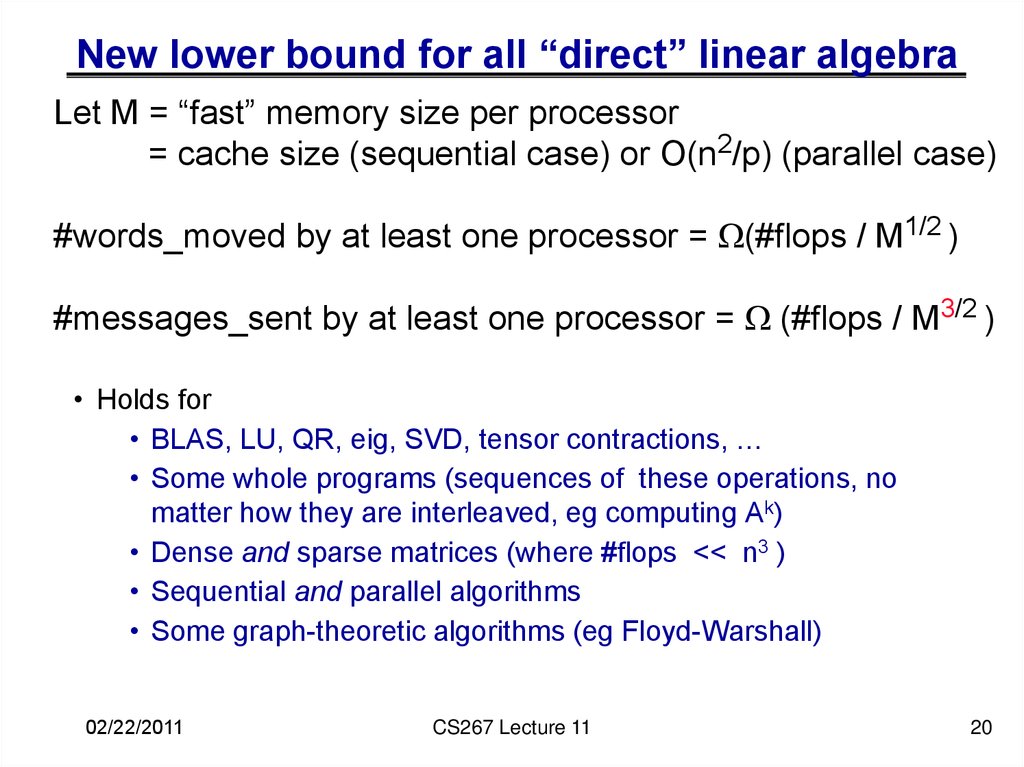
20. New lower bound for all “direct” linear algebra

Let M = “fast” memory size per processor
= cache size (sequential case) or O(n2/p) (parallel case)
#words_moved by at least one processor = (#flops / M1/2 )
#messages_sent by at least one processor = (#flops / M3/2 )
• Holds for
• BLAS, LU, QR, eig, SVD, tensor contractions, …
• Some whole programs (sequences of these operations, no
matter how they are interleaved, eg computing Ak)
• Dense and sparse matrices (where #flops << n3 )
• Sequential and parallel algorithms
• Some graph-theoretic algorithms (eg Floyd-Warshall)
02/22/2011
CS267 Lecture 11
20

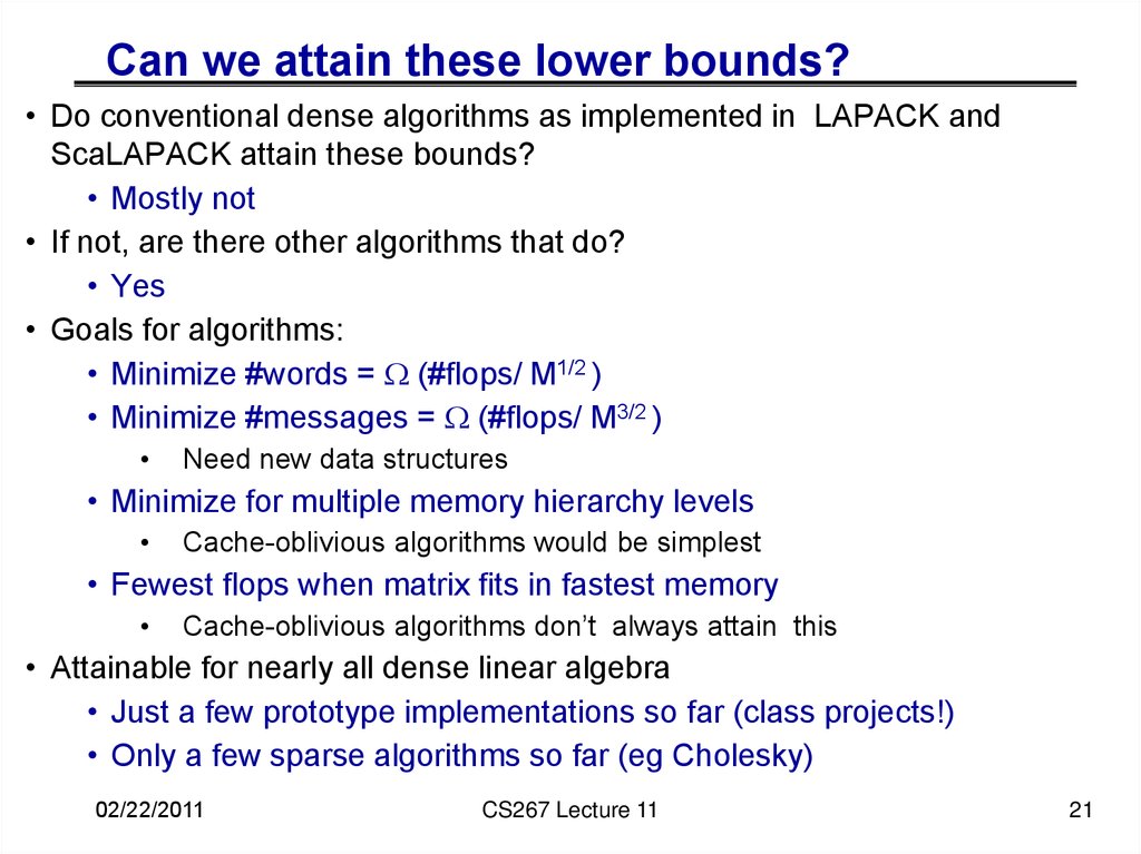
21. Can we attain these lower bounds?

• Do conventional dense algorithms as implemented in LAPACK and
ScaLAPACK attain these bounds?
• Mostly not
• If not, are there other algorithms that do?
• Yes
• Goals for algorithms:
• Minimize #words = (#flops/ M1/2 )
• Minimize #messages = (#flops/ M3/2 )
Need new data structures
• Minimize for multiple memory hierarchy levels
Cache-oblivious algorithms would be simplest
• Fewest flops when matrix fits in fastest memory
Cache-oblivious algorithms don’t always attain this
• Attainable for nearly all dense linear algebra
• Just a few prototype implementations so far (class projects!)
• Only a few sparse algorithms so far (eg Cholesky)
02/22/2011
CS267 Lecture 11
21

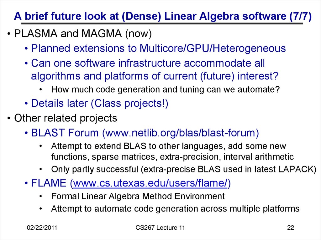
22. A brief future look at (Dense) Linear Algebra software (7/7)

• PLASMA and MAGMA (now)
• Planned extensions to Multicore/GPU/Heterogeneous
• Can one software infrastructure accommodate all
algorithms and platforms of current (future) interest?
• How much code generation and tuning can we automate?
• Details later (Class projects!)
• Other related projects
• BLAST Forum (www.netlib.org/blas/blast-forum)
• Attempt to extend BLAS to other languages, add some new
functions, sparse matrices, extra-precision, interval arithmetic
• Only partly successful (extra-precise BLAS used in latest LAPACK)
• FLAME (www.cs.utexas.edu/users/flame/)
• Formal Linear Algebra Method Environment
• Attempt to automate code generation across multiple platforms
02/22/2011
CS267 Lecture 11
22

23. Outline

History and motivation
Structure of the Dense Linear Algebra motif
Parallel Matrix-matrix multiplication
Parallel Gaussian Elimination (next time)
02/22/2011
CS267 Lecture 11
23

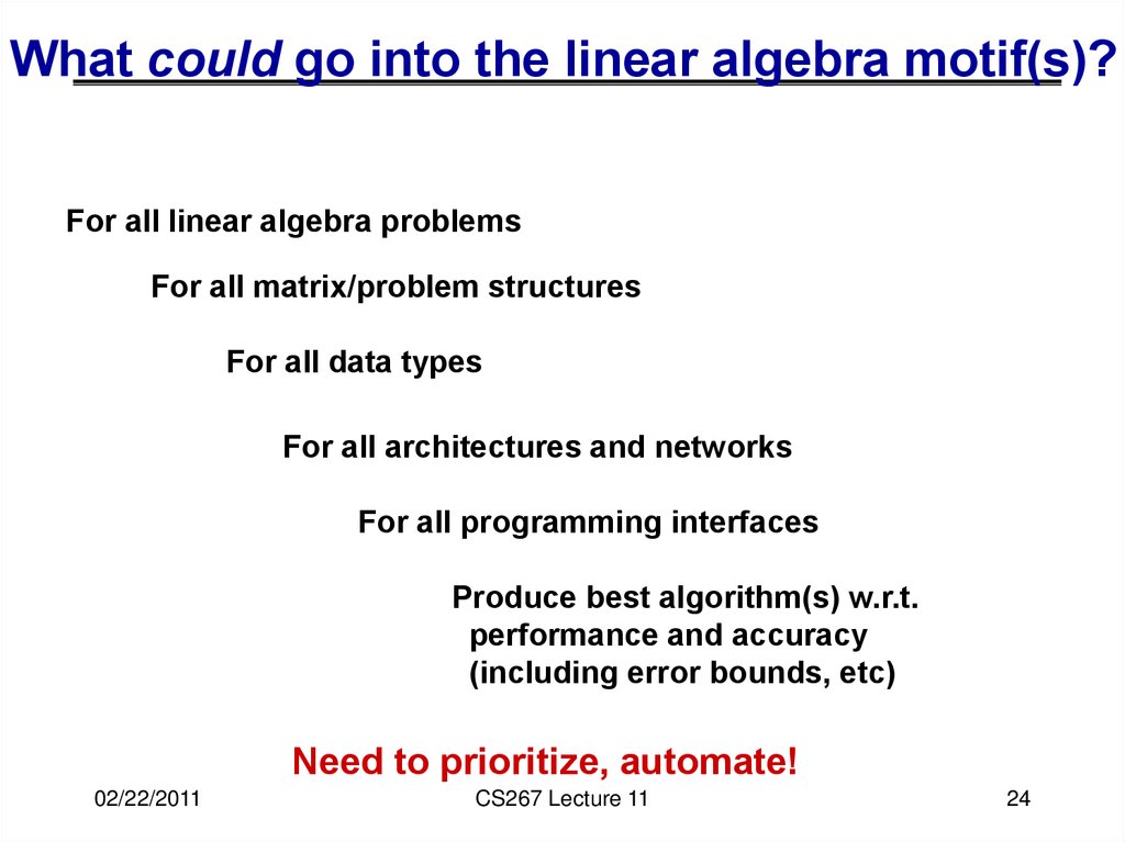
24. What could go into the linear algebra motif(s)?

For all linear algebra problems
For all matrix/problem structures
For all data types
For all architectures and networks
For all programming interfaces
Produce best algorithm(s) w.r.t.
performance and accuracy
(including error bounds, etc)
Need to prioritize, automate!
02/22/2011
CS267 Lecture 11
24

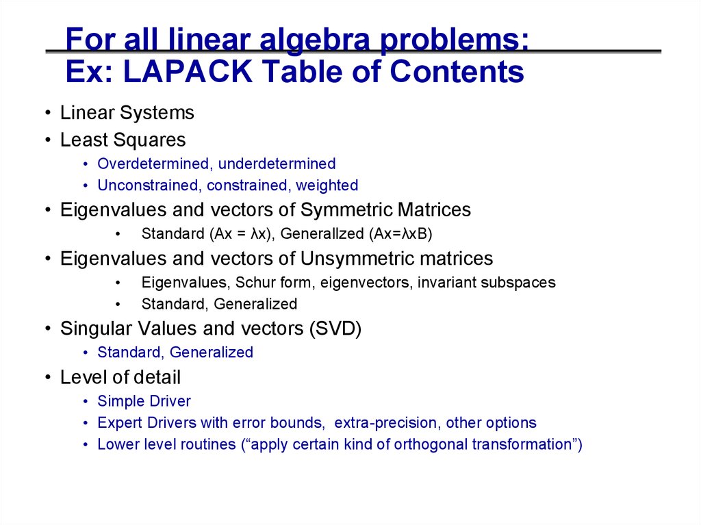
25. For all linear algebra problems: Ex: LAPACK Table of Contents

• Linear Systems
• Least Squares
• Overdetermined, underdetermined
• Unconstrained, constrained, weighted
• Eigenvalues and vectors of Symmetric Matrices
Standard (Ax = λx), Generalized (Ax=λBx)
• Eigenvalues and vectors of Unsymmetric matrices
Eigenvalues, Schur form, eigenvectors, invariant subspaces
Standard, Generalized
• Singular Values and vectors (SVD)
• Standard, Generalized
• Level of detail
• Simple Driver
• Expert Drivers with error bounds, extra-precision, other options
• Lower level routines (“apply certain kind of orthogonal transformation”)
02/22/2011
CS267 Lecture 11
25

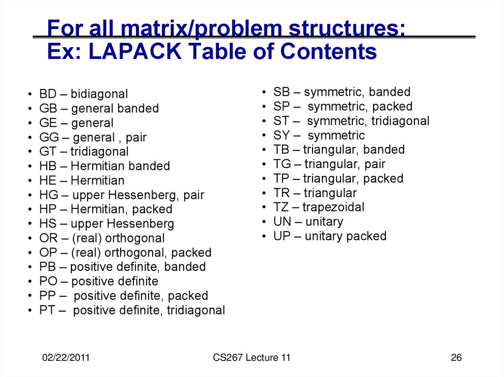
26. For all matrix/problem structures: Ex: LAPACK Table of Contents

BD – bidiagonal
GB – general banded
GE – general
GG – general , pair
GT – tridiagonal
HB – Hermitian banded
HE – Hermitian
HG – upper Hessenberg, pair
HP – Hermitian, packed
HS – upper Hessenberg
OR – (real) orthogonal
OP – (real) orthogonal, packed
PB – positive definite, banded
PO – positive definite
PP – positive definite, packed
PT – positive definite, tridiagonal
02/22/2011
SB – symmetric, banded
SP – symmetric, packed
ST – symmetric, tridiagonal
SY – symmetric
TB – triangular, banded
TG – triangular, pair
TP – triangular, packed
TR – triangular
TZ – trapezoidal
UN – unitary
UP – unitary packed
CS267 Lecture 11
26

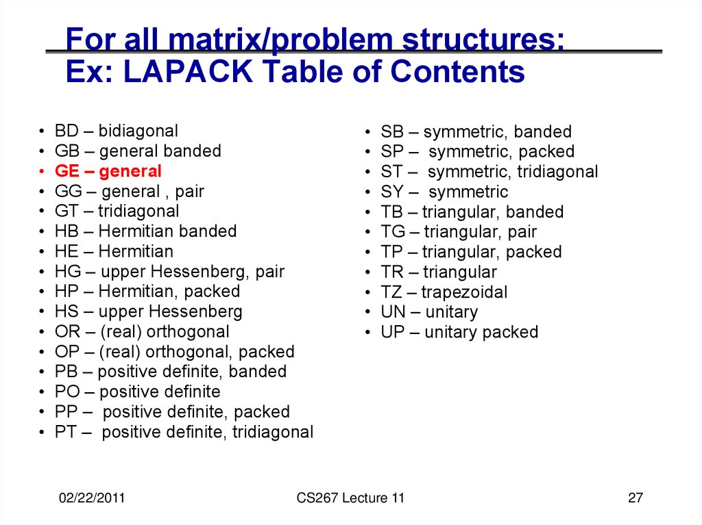
27. For all matrix/problem structures: Ex: LAPACK Table of Contents

BD – bidiagonal
GB – general banded
GE – general
GG – general , pair
GT – tridiagonal
HB – Hermitian banded
HE – Hermitian
HG – upper Hessenberg, pair
HP – Hermitian, packed
HS – upper Hessenberg
OR – (real) orthogonal
OP – (real) orthogonal, packed
PB – positive definite, banded
PO – positive definite
PP – positive definite, packed
PT – positive definite, tridiagonal
02/22/2011
SB – symmetric, banded
SP – symmetric, packed
ST – symmetric, tridiagonal
SY – symmetric
TB – triangular, banded
TG – triangular, pair
TP – triangular, packed
TR – triangular
TZ – trapezoidal
UN – unitary
UP – unitary packed
CS267 Lecture 11
27

28. For all matrix/problem structures: Ex: LAPACK Table of Contents

BD – bidiagonal
GB – general banded
GE – general
GG – general, pair
GT – tridiagonal
HB – Hermitian banded
HE – Hermitian
HG – upper Hessenberg, pair
HP – Hermitian, packed
HS – upper Hessenberg
OR – (real) orthogonal
OP – (real) orthogonal, packed
PB – positive definite, banded
PO – positive definite
PP – positive definite, packed
PT – positive definite, tridiagonal
02/22/2011
SB – symmetric, banded
SP – symmetric, packed
ST – symmetric, tridiagonal
SY – symmetric
TB – triangular, banded
TG – triangular, pair
TP – triangular, packed
TR – triangular
TZ – trapezoidal
UN – unitary
UP – unitary packed
CS267 Lecture 11
28

29. For all matrix/problem structures: Ex: LAPACK Table of Contents

BD – bidiagonal
GB – general banded
GE – general
GG – general, pair
GT – tridiagonal
HB – Hermitian banded
HE – Hermitian
HG – upper Hessenberg, pair
HP – Hermitian, packed
HS – upper Hessenberg
OR – (real) orthogonal
OP – (real) orthogonal, packed
PB – positive definite, banded
PO – positive definite
PP – positive definite, packed
PT – positive definite, tridiagonal
02/22/2011
SB – symmetric, banded
SP – symmetric, packed
ST – symmetric, tridiagonal
SY – symmetric
TB – triangular, banded
TG – triangular, pair
TP – triangular, packed
TR – triangular
TZ – trapezoidal
UN – unitary
UP – unitary packed
CS267 Lecture 11
29

30. For all matrix/problem structures: Ex: LAPACK Table of Contents

BD – bidiagonal
GB – general banded
GE – general
GG – general, pair
GT – tridiagonal
HB – Hermitian banded
HE – Hermitian
HG – upper Hessenberg, pair
HP – Hermitian, packed
HS – upper Hessenberg
OR – (real) orthogonal
OP – (real) orthogonal, packed
PB – positive definite, banded
PO – positive definite
PP – positive definite, packed
PT – positive definite, tridiagonal
02/22/2011
SB – symmetric, banded
SP – symmetric, packed
ST – symmetric, tridiagonal
SY – symmetric
TB – triangular, banded
TG – triangular, pair
TP – triangular, packed
TR – triangular
TZ – trapezoidal
UN – unitary
UP – unitary packed
CS267 Lecture 11
30

31. For all matrix/problem structures: Ex: LAPACK Table of Contents

BD – bidiagonal
GB – general banded
GE – general
GG – general, pair
GT – tridiagonal
HB – Hermitian banded
HE – Hermitian
HG – upper Hessenberg, pair
HP – Hermitian, packed
HS – upper Hessenberg
OR – (real) orthogonal
OP – (real) orthogonal, packed
PB – positive definite, banded
PO – positive definite
PP – positive definite, packed
PT – positive definite, tridiagonal
02/22/2011
SB – symmetric, banded
SP – symmetric, packed
ST – symmetric, tridiagonal
SY – symmetric
TB – triangular, banded
TG – triangular, pair
TP – triangular, packed
TR – triangular
TZ – trapezoidal
UN – unitary
UP – unitary packed
CS267 Lecture 11
31

32. For all matrix/problem structures: Ex: LAPACK Table of Contents

BD – bidiagonal
GB – general banded
GE – general
GG – general , pair
GT – tridiagonal
HB – Hermitian banded
HE – Hermitian
HG – upper Hessenberg, pair
HP – Hermitian, packed
HS – upper Hessenberg
OR – (real) orthogonal
OP – (real) orthogonal, packed
PB – positive definite, banded
PO – positive definite
PP – positive definite, packed
PT – positive definite, tridiagonal
02/22/2011
SB – symmetric, banded
SP – symmetric, packed
ST – symmetric, tridiagonal
SY – symmetric
TB – triangular, banded
TG – triangular, pair
TP – triangular, packed
TR – triangular
TZ – trapezoidal
UN – unitary
UP – unitary packed
CS267 Lecture 11
32

33. For all matrix/problem structures: Ex: LAPACK Table of Contents

BD – bidiagonal
GB – general banded
GE – general
GG – general, pair
GT – tridiagonal
HB – Hermitian banded
HE – Hermitian
HG – upper Hessenberg, pair
HP – Hermitian, packed
HS – upper Hessenberg
OR – (real) orthogonal
OP – (real) orthogonal, packed
PB – positive definite, banded
PO – positive definite
PP – positive definite, packed
PT – positive definite, tridiagonal
02/22/2011
SB – symmetric, banded
SP – symmetric, packed
ST – symmetric, tridiagonal
SY – symmetric
TB – triangular, banded
TG – triangular, pair
TP – triangular, packed
TR – triangular
TZ – trapezoidal
UN – unitary
UP – unitary packed
CS267 Lecture 11
33

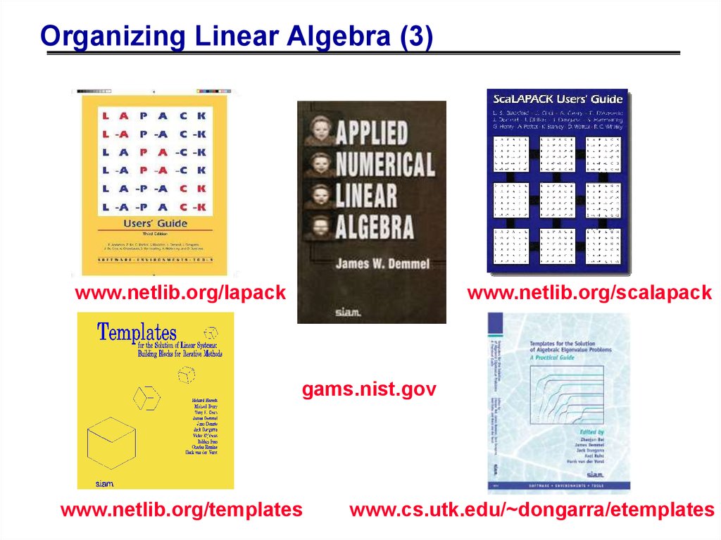
34. Organizing Linear Algebra – in books

www.netlib.org/lapack
www.netlib.org/scalapack
gams.nist.gov
www.netlib.org/templates
www.cs.utk.edu/~dongarra/etemplates

35. Outline

History and motivation
Structure of the Dense Linear Algebra motif
Parallel Matrix-matrix multiplication
Parallel Gaussian Elimination (next time)
02/22/2011
CS267 Lecture 11
35

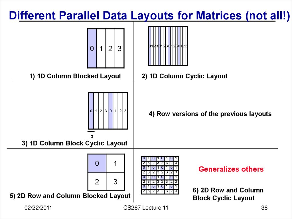
36. Different Parallel Data Layouts for Matrices (not all!)

0123012301230123
0 1 2 3
1) 1D Column Blocked Layout
2) 1D Column Cyclic Layout
0 1 2 3 0 1 2 3
4) Row versions of the previous layouts
b
3) 1D Column Block Cyclic Layout
0
1
2
3
0
2
0
2
0
2
0
2
1
3
1
3
1
3
1
3
0
2
0
2
0
2
0
2
1
3
1
3
1
3
1
3
0
2
0
2
0
2
0
2
1
3
1
3
1
3
1
3
5) 2D Row and Column Blocked Layout
02/22/2011
CS267 Lecture 11
0
2
0
2
0
2
0
2
1
3
1
3
1
3
1
3
Generalizes others
6) 2D Row and Column
Block Cyclic Layout
36

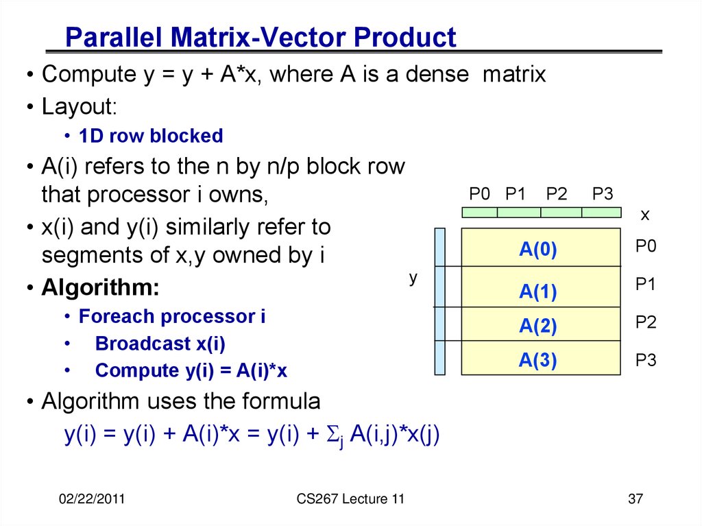
37. Parallel Matrix-Vector Product

• Compute y = y + A*x, where A is a dense matrix
• Layout:
• 1D row blocked
• A(i) refers to the n by n/p block row
that processor i owns,
• x(i) and y(i) similarly refer to
segments of x,y owned by i
y
• Algorithm:
• Foreach processor i
• Broadcast x(i)
• Compute y(i) = A(i)*x
P0 P1
P2
P3
x
A(0)
P0
A(1)
P1
A(2)
P2
A(3)
P3
• Algorithm uses the formula
y(i) = y(i) + A(i)*x = y(i) + Sj A(i,j)*x(j)
02/22/2011
CS267 Lecture 11
37

38. Matrix-Vector Product y = y + A*x

• A column layout of the matrix eliminates the broadcast of x
• But adds a reduction to update the destination y
• A 2D blocked layout uses a broadcast and reduction, both
on a subset of processors
• sqrt(p) for square processor grid
02/22/2011
P0
P1
P2
P3
P0
P1
P2
P3
P4
P5
P6
P7
P8
P9
P10 P11
P12
P13 P14 P15
CS267 Lecture 11
38

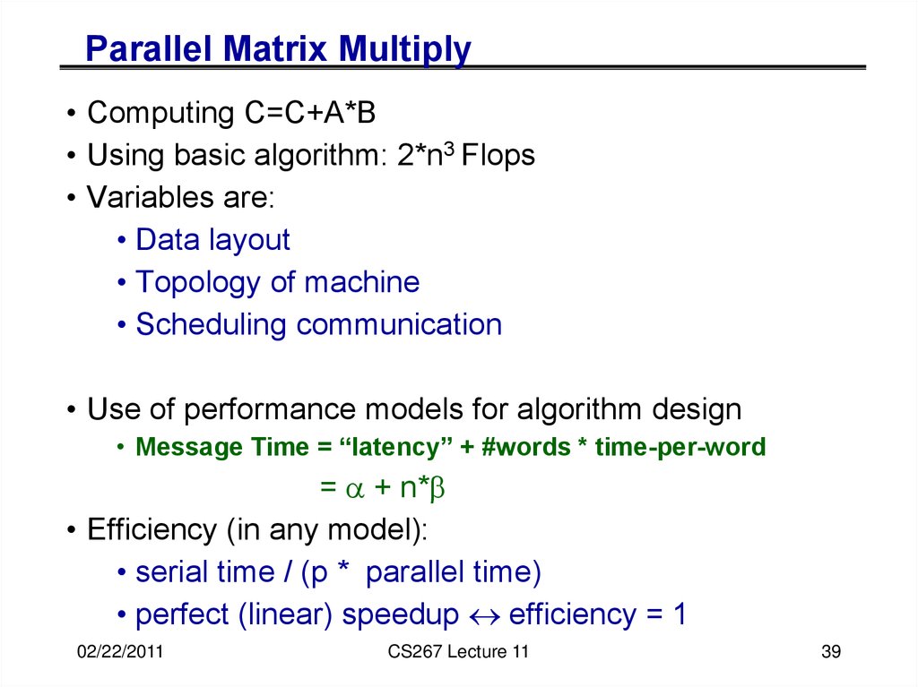
39. Parallel Matrix Multiply

• Computing C=C+A*B
• Using basic algorithm: 2*n3 Flops
• Variables are:
• Data layout
• Topology of machine
• Scheduling communication
• Use of performance models for algorithm design
• Message Time = “latency” + #words * time-per-word
= a + n*b
• Efficiency (in any model):
• serial time / (p * parallel time)
• perfect (linear) speedup efficiency = 1
02/22/2011
CS267 Lecture 11
39

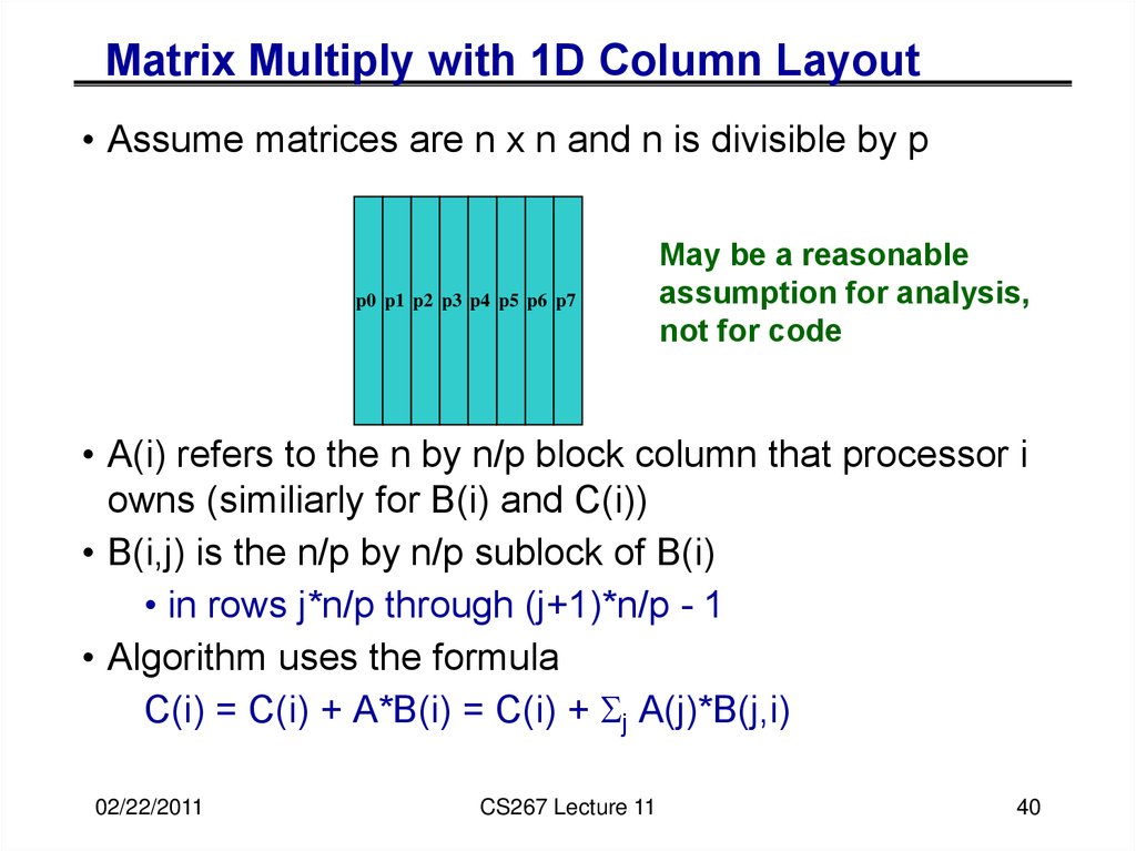
40. Matrix Multiply with 1D Column Layout

• Assume matrices are n x n and n is divisible by p
p0 p1 p2 p3 p4 p5 p6 p7
May be a reasonable
assumption for analysis,
not for code
• A(i) refers to the n by n/p block column that processor i
owns (similiarly for B(i) and C(i))
• B(i,j) is the n/p by n/p sublock of B(i)
• in rows j*n/p through (j+1)*n/p - 1
• Algorithm uses the formula
C(i) = C(i) + A*B(i) = C(i) + Sj A(j)*B(j,i)
02/22/2011
CS267 Lecture 11
40

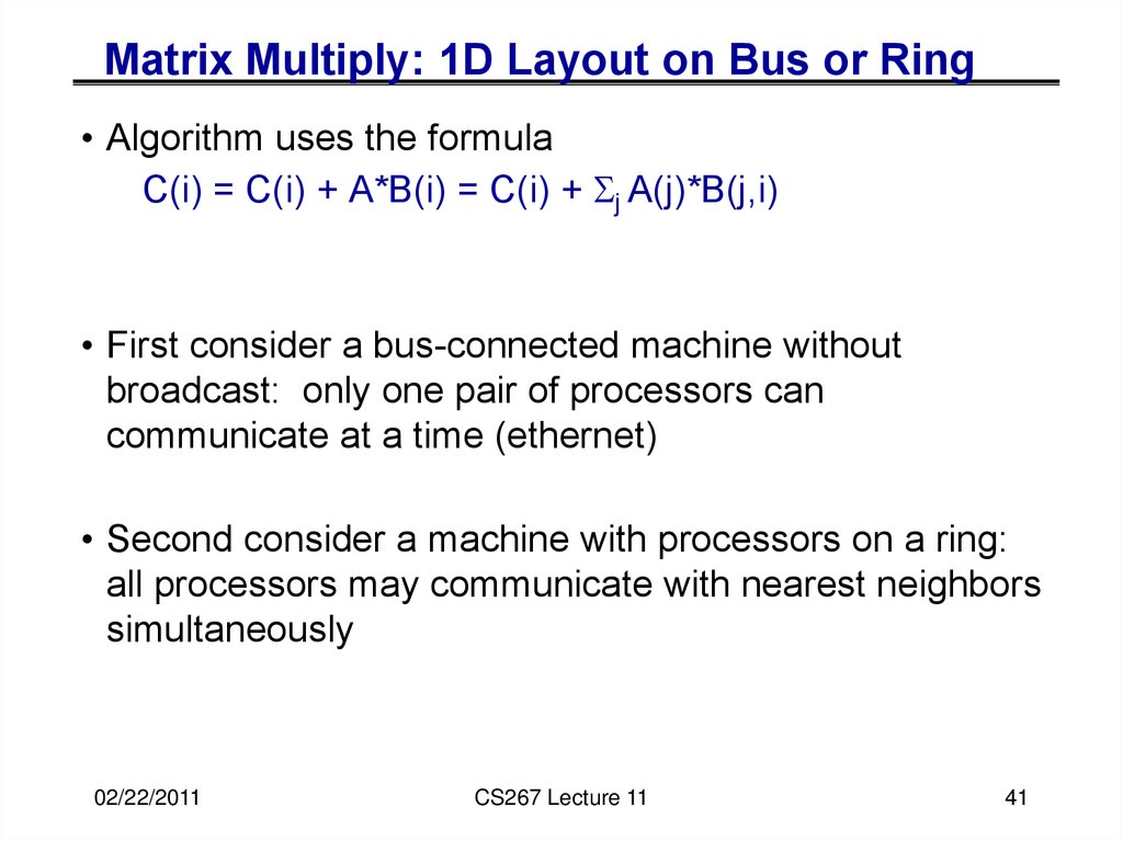
41. Matrix Multiply: 1D Layout on Bus or Ring

• Algorithm uses the formula
C(i) = C(i) + A*B(i) = C(i) + Sj A(j)*B(j,i)
• First consider a bus-connected machine without
broadcast: only one pair of processors can
communicate at a time (ethernet)
• Second consider a machine with processors on a ring:
all processors may communicate with nearest neighbors
simultaneously
02/22/2011
CS267 Lecture 11
41

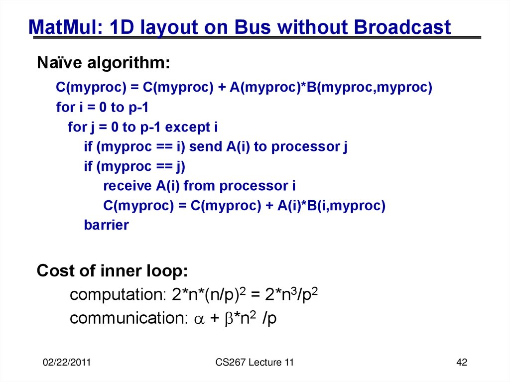
42. MatMul: 1D layout on Bus without Broadcast

Naïve algorithm:
C(myproc) = C(myproc) + A(myproc)*B(myproc,myproc)
for i = 0 to p-1
for j = 0 to p-1 except i
if (myproc == i) send A(i) to processor j
if (myproc == j)
receive A(i) from processor i
C(myproc) = C(myproc) + A(i)*B(i,myproc)
barrier
Cost of inner loop:
computation: 2*n*(n/p)2 = 2*n3/p2
communication: a + b*n2 /p
02/22/2011
CS267 Lecture 11
42

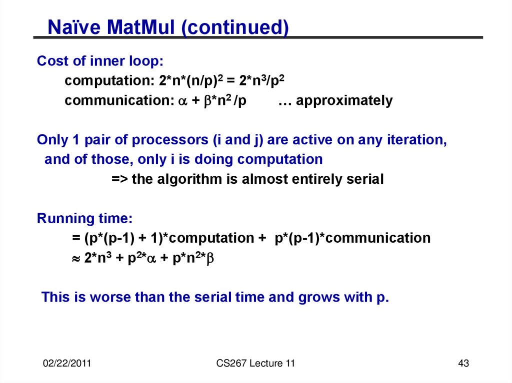
43. Naïve MatMul (continued)

Cost of inner loop:
computation: 2*n*(n/p)2 = 2*n3/p2
communication: a + b*n2 /p
… approximately
Only 1 pair of processors (i and j) are active on any iteration,
and of those, only i is doing computation
=> the algorithm is almost entirely serial
Running time:
= (p*(p-1) + 1)*computation + p*(p-1)*communication
2*n3 + p2*a + p*n2*b
This is worse than the serial time and grows with p.
02/22/2011
CS267 Lecture 11
43

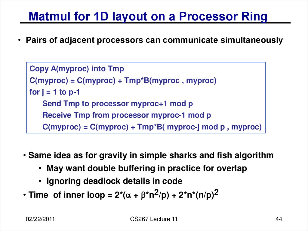
44. Matmul for 1D layout on a Processor Ring

• Pairs of adjacent processors can communicate simultaneously
Copy A(myproc) into Tmp
C(myproc) = C(myproc) + Tmp*B(myproc , myproc)
for j = 1 to p-1
Send Tmp to processor myproc+1 mod p
Receive Tmp from processor myproc-1 mod p
C(myproc) = C(myproc) + Tmp*B( myproc-j mod p , myproc)
• Same idea as for gravity in simple sharks and fish algorithm
• May want double buffering in practice for overlap
• Ignoring deadlock details in code
• Time of inner loop = 2*(a + b*n2/p) + 2*n*(n/p)2
02/22/2011
CS267 Lecture 11
44

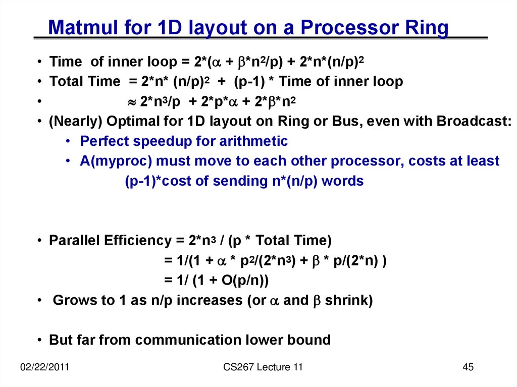
45. Matmul for 1D layout on a Processor Ring

• Time of inner loop = 2*(a + b*n2/p) + 2*n*(n/p)2
• Total Time = 2*n* (n/p)2 + (p-1) * Time of inner loop
2*n3/p + 2*p*a + 2*b*n2
• (Nearly) Optimal for 1D layout on Ring or Bus, even with Broadcast:
• Perfect speedup for arithmetic
• A(myproc) must move to each other processor, costs at least
(p-1)*cost of sending n*(n/p) words
• Parallel Efficiency = 2*n3 / (p * Total Time)
= 1/(1 + a * p2/(2*n3) + b * p/(2*n) )
= 1/ (1 + O(p/n))
• Grows to 1 as n/p increases (or a and b shrink)
• But far from communication lower bound
02/22/2011
CS267 Lecture 11
45

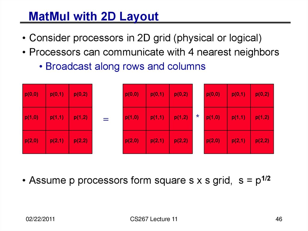
46. MatMul with 2D Layout

• Consider processors in 2D grid (physical or logical)
• Processors can communicate with 4 nearest neighbors
• Broadcast along rows and columns
p(0,0)
p(0,1)
p(0,2)
p(1,0)
p(1,1)
p(1,2)
p(2,0)
p(2,1)
p(2,2)
=
p(0,0)
p(0,1)
p(0,2)
p(1,0)
p(1,1)
p(1,2)
p(2,0)
p(2,1)
p(2,2)
*
p(0,0)
p(0,1)
p(0,2)
p(1,0)
p(1,1)
p(1,2)
p(2,0)
p(2,1)
p(2,2)
• Assume p processors form square s x s grid, s = p1/2
02/22/2011
CS267 Lecture 11
46

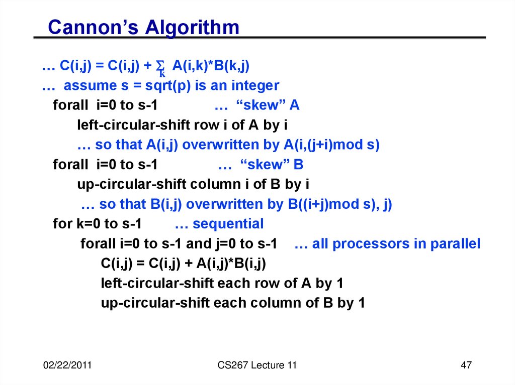
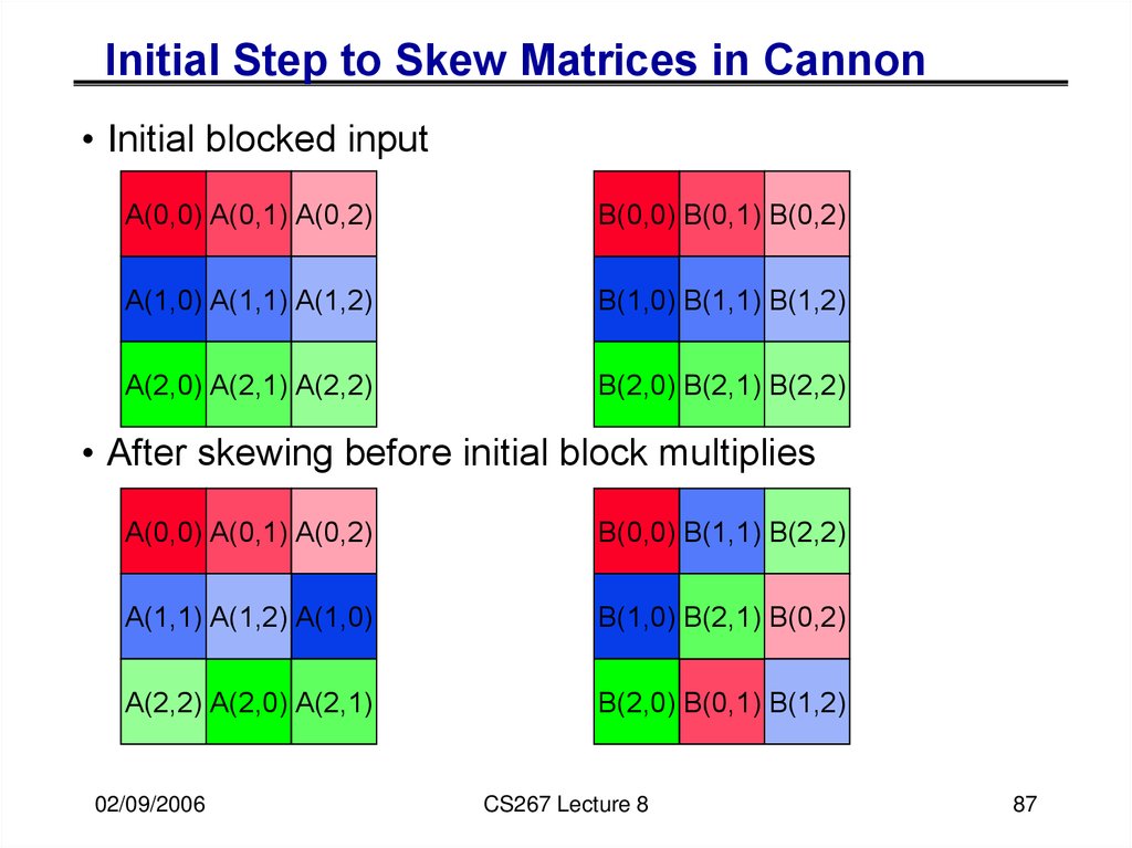
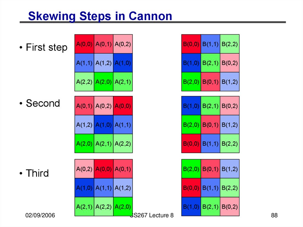
47. Cannon’s Algorithm

… C(i,j) = C(i,j) + Sk A(i,k)*B(k,j)
… assume s = sqrt(p) is an integer
forall i=0 to s-1
… “skew” A
left-circular-shift row i of A by i
… so that A(i,j) overwritten by A(i,(j+i)mod s)
forall i=0 to s-1
… “skew” B
up-circular-shift column i of B by i
… so that B(i,j) overwritten by B((i+j)mod s), j)
for k=0 to s-1
… sequential
forall i=0 to s-1 and j=0 to s-1 … all processors in parallel
C(i,j) = C(i,j) + A(i,j)*B(i,j)
left-circular-shift each row of A by 1
up-circular-shift each column of B by 1
02/22/2011
CS267 Lecture 11
47

48. Cannon’s Matrix Multiplication

C(1,2) = A(1,0) * B(0,2) + A(1,1) * B(1,2) + A(1,2) * B(2,2)
02/22/2011
CS267 Lecture 11
48

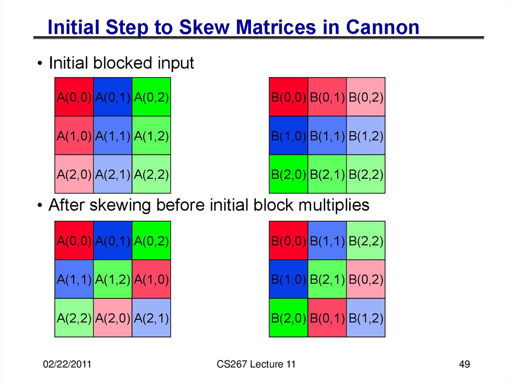
49. Initial Step to Skew Matrices in Cannon

• Initial blocked input
A(0,0) A(0,1) A(0,2)
B(0,0) B(0,1) B(0,2)
A(1,0) A(1,1) A(1,2)
B(1,0) B(1,1) B(1,2)
A(2,0) A(2,1) A(2,2)
B(2,0) B(2,1) B(2,2)
• After skewing before initial block multiplies
A(0,0) A(0,1) A(0,2)
B(0,0) B(1,1) B(2,2)
A(1,1) A(1,2) A(1,0)
B(1,0) B(2,1) B(0,2)
A(2,2) A(2,0) A(2,1)
B(2,0) B(0,1) B(1,2)
02/22/2011
CS267 Lecture 11
49

50. Skewing Steps in Cannon All blocks of A must multiply all like-colored blocks of B

• First step
• Second
• Third
02/22/2011
A(0,0) A(0,1) A(0,2)
B(0,0) B(1,1) B(2,2)
A(1,1) A(1,2) A(1,0)
B(1,0) B(2,1) B(0,2)
A(2,2) A(2,0) A(2,1)
B(2,0) B(0,1) B(1,2)
A(0,1) A(0,2) A(0,0)
B(1,0) B(2,1) B(0,2)
A(1,2) A(1,0) A(1,1)
B(2,0) B(0,1) B(1,2)
A(2,0) A(2,1) A(2,2)
B(0,0) B(1,1) B(2,2)
A(0,2) A(0,0) A(0,1)
B(2,0) B(0,1) B(1,2)
A(1,0) A(1,1) A(1,2)
B(0,0) B(1,1) B(2,2)
A(2,1) A(2,2) A(2,0)
B(1,0) B(2,1) B(0,2)
CS267 Lecture 11
50

51. Cost of Cannon’s Algorithm

forall i=0 to s-1
… recall s = sqrt(p)
left-circular-shift row i of A by i … cost ≤ s*(a + b*n2/p)
forall i=0 to s-1
up-circular-shift column i of B by i … cost ≤ s*(a + b*n2/p)
for k=0 to s-1
forall i=0 to s-1 and j=0 to s-1
C(i,j) = C(i,j) + A(i,j)*B(i,j) … cost = 2*(n/s)3 = 2*n3/p3/2
left-circular-shift each row of A by 1 … cost = a + b*n2/p
up-circular-shift each column of B by 1 … cost = a + b*n2/p
° Total Time = 2*n3/p + 4* s*a + 4*b*n2/s - Optimal!
° Parallel Efficiency = 2*n3 / (p * Total Time)
= 1/( 1 + a * 2*(s/n)3 + b * 2*(s/n) )
= 1/(1 + O(sqrt(p)/n))
° Grows to 1 as n/s = n/sqrt(p) = sqrt(data per processor) grows
° Better than 1D layout, which had Efficiency = 1/(1 + O(p/n))
02/22/2011
CS267 Lecture 11
51

52. Cannon’s Algorithm is “optimal”

Pros and Cons of Cannon
• So what if it’s “optimal”, is it fast?
• Local computation one call to (optimized) matrix-multiply
• Hard to generalize for
• p not a perfect square
• A and B not square
• Dimensions of A, B not perfectly divisible by
s=sqrt(p)
• A and B not “aligned” in the way they are stored on
processors
• block-cyclic layouts
• Needs extra memory for copies of local matrices
02/22/2011
CS267 Lecture 11
53

53. Pros and Cons of Cannon

SUMMA Algorithm
• SUMMA = Scalable Universal Matrix Multiply
• Slightly less efficient, but simpler and easier to generalize
• Presentation from van de Geijn and Watts
• www.netlib.org/lapack/lawns/lawn96.ps
• Similar ideas appeared many times
• Used in practice in PBLAS = Parallel BLAS
• www.netlib.org/lapack/lawns/lawn100.ps
02/22/2011
CS267 Lecture 11
54

54. SUMMA Algorithm

SUMMA
k
j
B(k,j)
k
i
*
=
C(i,j)
A(i,k)
i, j represent all rows, columns owned by a processor
• k is a block of b 1 rows or columns
• C(i,j) = C(i,j) + Sk A(i,k)*B(k,j)
• Assume a pr by pc processor grid (pr = pc = 4 above)
• Need not be square
02/22/2011
CS267 Lecture 11
55

55. SUMMA

k
j
B(k,j)
k
*
i
=
C(i,j)
A(i,k)
For k=0 to n/b-1
… where b is the block size
… b = # cols in A(i,k) and # rows in B(k,j)
for all i = 1 to pr … in parallel
owner of A(i,k) broadcasts it to whole processor row
for all j = 1 to pc … in parallel
owner of B(k,j) broadcasts it to whole processor column
Receive A(i,k) into Acol
Receive B(k,j) into Brow
C_myproc = C_myproc + Acol * Brow
02/22/2011
CS267 Lecture 11
56

56. SUMMA

performance
° To simplify analysis only, assume s = sqrt(p)
For k=0 to n/b-1
for all i = 1 to s … s = sqrt(p)
owner of A(i,k) broadcasts it to whole processor row
… time = log s *( a + b * b*n/s), using a tree
for all j = 1 to s
owner of B(k,j) broadcasts it to whole processor column
… time = log s *( a + b * b*n/s), using a tree
Receive A(i,k) into Acol
Receive B(k,j) into Brow
C_myproc = C_myproc + Acol * Brow
… time = 2*(n/s)2*b
° Total time = 2*n3/p + a * log p * n/b + b * log p * n2 /s
02/22/2011
CS267 Lecture 11
57

57. SUMMA performance

• Total time = 2*n3/p + a * log p * n/b + b * log p * n2 /s
• Parallel Efficiency =
1/(1 + a * log p * p / (2*b*n2) + b * log p * s/(2*n) )
• Same b term as Cannon, except for log p factor
log p grows slowly so this is ok
• Latency (a) term can be larger, depending on b
When b=1, get a * log p * n
As b grows to n/s, term shrinks to
a * log p * s (log p times Cannon)
• Temporary storage grows like 2*b*n/s
• Can change b to tradeoff latency cost with memory
02/22/2011
CS267 Lecture 11
58

58. SUMMA performance

PDGEMM = PBLAS routine
for matrix multiply
Observations:
For fixed N, as P increases
Mflops increases, but
less than 100% efficiency
For fixed P, as N increases,
Mflops (efficiency) rises
DGEMM = BLAS routine
for matrix multiply
Maximum speed for PDGEMM
= # Procs * speed of DGEMM
Observations (same as above):
Efficiency always at least 48%
For fixed N, as P increases,
efficiency drops
For fixed P, as N increases,
efficiency increases
02/22/2011
CS267 Lecture 8
59

59.

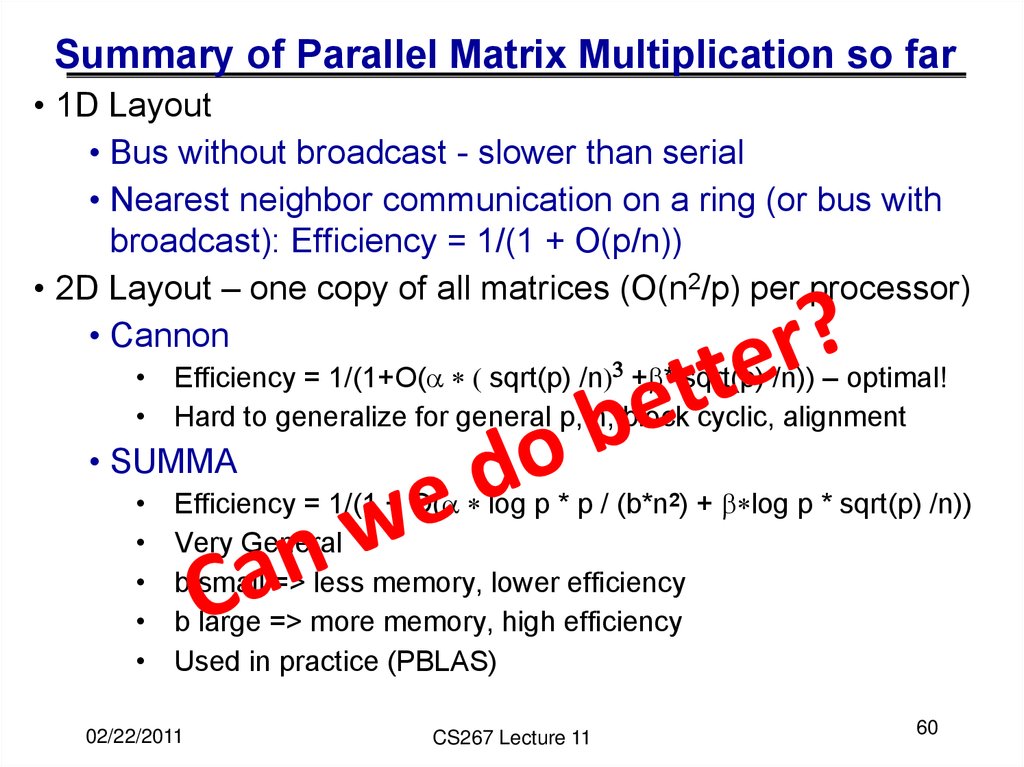
Summary of Parallel Matrix Multiplication so far
• 1D Layout
• Bus without broadcast - slower than serial
• Nearest neighbor communication on a ring (or bus with
broadcast): Efficiency = 1/(1 + O(p/n))
• 2D Layout – one copy of all matrices (O(n2/p) per processor)
• Cannon
• Efficiency = 1/(1+O(a * ( sqrt(p) /n)3 +b* sqrt(p) /n)) – optimal!
• Hard to generalize for general p, n, block cyclic, alignment
• SUMMA
Efficiency = 1/(1 + O(a * log p * p / (b*n2) + b*log p * sqrt(p) /n))
Very General
b small => less memory, lower efficiency
b large => more memory, high efficiency
Used in practice (PBLAS)
02/22/2011
CS267 Lecture 11
60

60. Summary of Parallel Matrix Multiplication so far

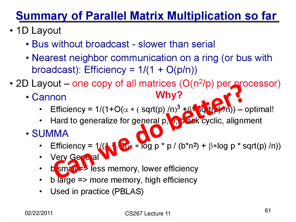
• 1D Layout
• Bus without broadcast - slower than serial
• Nearest neighbor communication on a ring (or bus with
broadcast): Efficiency = 1/(1 + O(p/n))
• 2D Layout – one copy of all matrices (O(n2/p) per processor)
Why?
• Cannon
• Efficiency = 1/(1+O(a * ( sqrt(p) /n)3 +b* sqrt(p) /n)) – optimal!
• Hard to generalize for general p, n, block cyclic, alignment
• SUMMA
Efficiency = 1/(1 + O(a * log p * p / (b*n2) + b*log p * sqrt(p) /n))
Very General
b small => less memory, lower efficiency
b large => more memory, high efficiency
Used in practice (PBLAS)
02/22/2011
CS267 Lecture 11
61

61. Summary of Parallel Matrix Multiplication so far

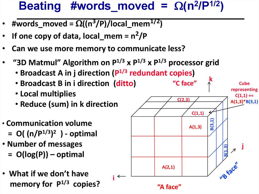
Beating #words_moved = (n2/P1/2)
• #words_moved = ((n3/P)/local_mem1/2)
• If one copy of data, local_mem = n2/P
• Can we use more memory to communicate less?
• “3D Matmul” Algorithm on P1/3 x P1/3 x P1/3 processor grid
• Broadcast A in j direction (P1/3 redundant copies)
k
“C face”
• Broadcast B in i direction (ditto)
• Local multiplies
C(2,3)
• Reduce (sum) in k direction
Cube
representing
C(1,1) +=
A(1,3)*B(3,1)
• Communication volume
A(1,3)
(n/P1/3)2
• What if we don’t have
memory for P1/3 copies?
B(1,3)
= O(
) - optimal
• Number of messages
= O(log(P)) – optimal
B(3,1)
C(1,1)
A(2,1)
i
“A face”
j

62. Beating #words_moved = (n2/P1/2)

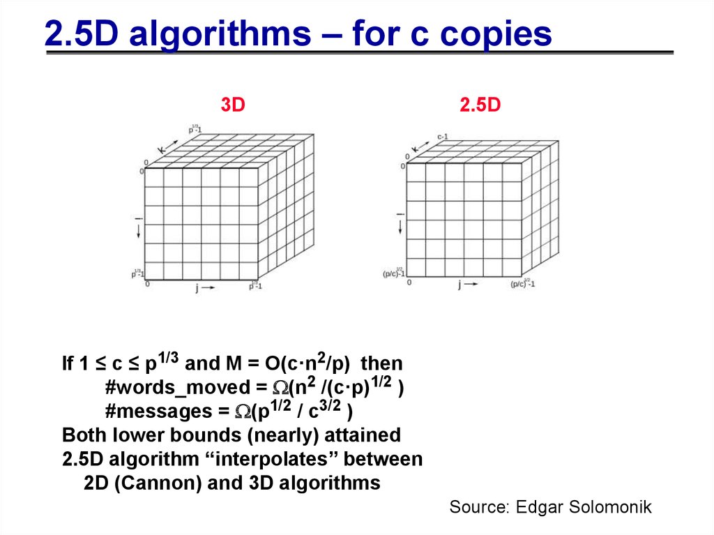
2.5D algorithms – for c copies
3D
2.5D
If 1 ≤ c ≤ p1/3 and M = O(c·n2/p) then
#words_moved = (n2 /(c·p)1/2 )
#messages = (p1/2 / c3/2 )
Both lower bounds (nearly) attained
2.5D algorithm “interpolates” between
2D (Cannon) and 3D algorithms
Source: Edgar Solomonik

63. 2.5D algorithms – for c copies

2.5D matrix multiply
• Interpolate between
Cannon and 3D matmul
• Replicate A, B c-1 times
• Do p1/2/c3/2 steps of Cannon
on each copy of A,B
• Sum contributions to C
from all c layers
• #words_moved = O( n2 / (cp)1/2 )
• #messages = O( p1/2/c3/2 + log(c) )
Source: Edgar Solomonik

64. 2.5D matrix multiply

performance
Source: Edgar Solomonik

65. 2.5D matrix multiply performance

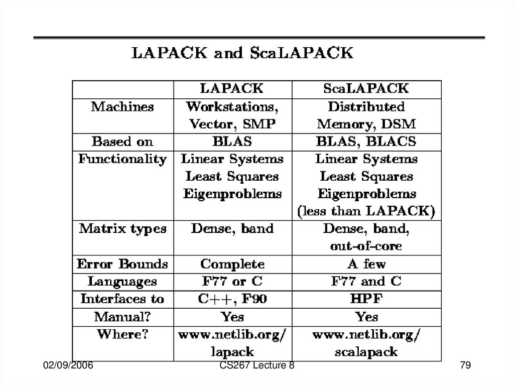
ScaLAPACK Parallel Library
02/22/2011
CS267 Lecture 11
66

66.

Extra Slides
02/22/2011
CS267 Lecture 11
67

67.

Recursive Layouts
• For both cache hierarchies and parallelism, recursive
layouts may be useful
• Z-Morton, U-Morton, and X-Morton Layout
• Also Hilbert layout and others
• What about the user’s view?
• Fortunately, many problems can be solved on a
permutation
• Never need to actually change the user’s layout
2/27/08
CS267 Guest Lecture 1
68

68. Recursive Layouts

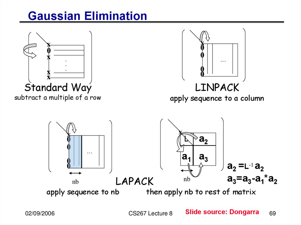
Gaussian Elimination
x
0
x
x
x
x
0
0
.
.
.
0
0
Standard Way
LINPACK
apply sequence to a column
subtract a multiple of a row
x
x
0
0
...
nb
L
a2
a1 a3
0
0
LAPACK
apply sequence to nb
02/09/2006
...
nb
a2 =L-1 a2
a3=a3-a1*a2
then apply nb to rest of matrix
CS267 Lecture 8
Slide source: Dongarra
69

69. Gaussian Elimination

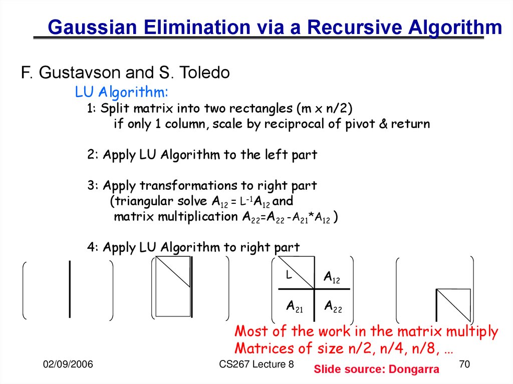
via a Recursive Algorithm
F. Gustavson and S. Toledo
LU Algorithm:
1: Split matrix into two rectangles (m x n/2)
if only 1 column, scale by reciprocal of pivot & return
2: Apply LU Algorithm to the left part
3: Apply transformations to right part
(triangular solve A12 = L-1A12 and
matrix multiplication A22=A22 -A21*A12 )
4: Apply LU Algorithm to right part
L
A12
A21
A22
Most of the work in the matrix multiply
Matrices of size n/2, n/4, n/8, …
02/09/2006
CS267 Lecture 8
Slide source: Dongarra
70

70. Gaussian Elimination via a Recursive Algorithm

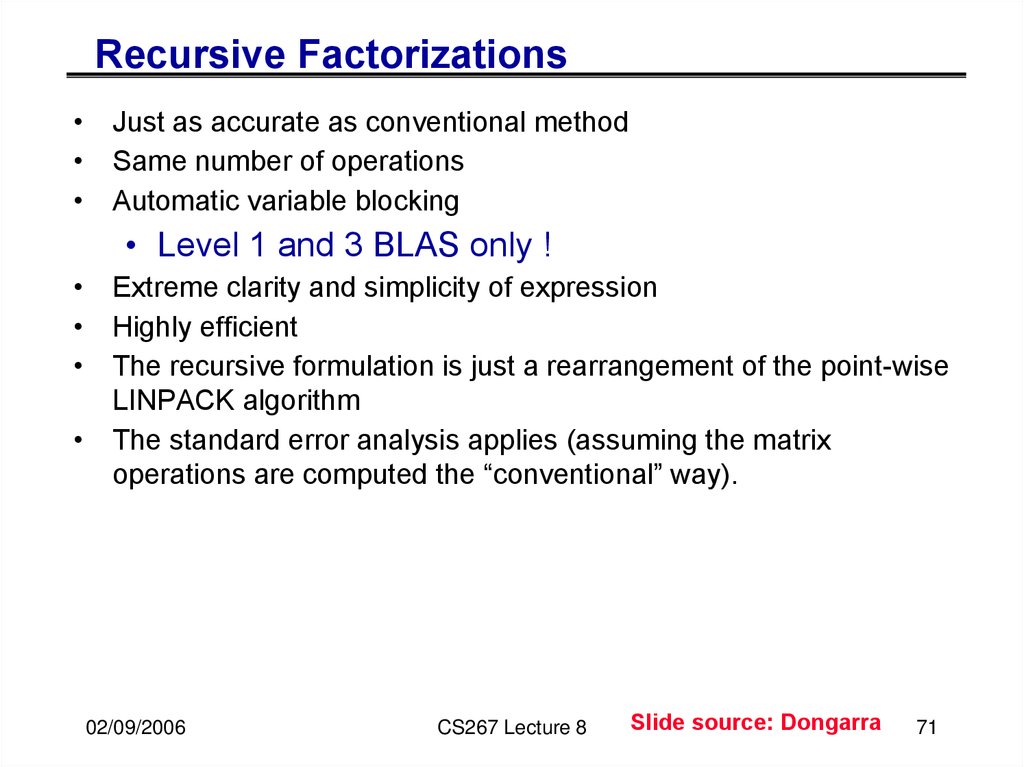
Recursive Factorizations
• Just as accurate as conventional method
• Same number of operations
• Automatic variable blocking
• Level 1 and 3 BLAS only !
• Extreme clarity and simplicity of expression
• Highly efficient
• The recursive formulation is just a rearrangement of the point-wise
LINPACK algorithm
• The standard error analysis applies (assuming the matrix
operations are computed the “conventional” way).
02/09/2006
CS267 Lecture 8
Slide source: Dongarra
71

71. Recursive Factorizations

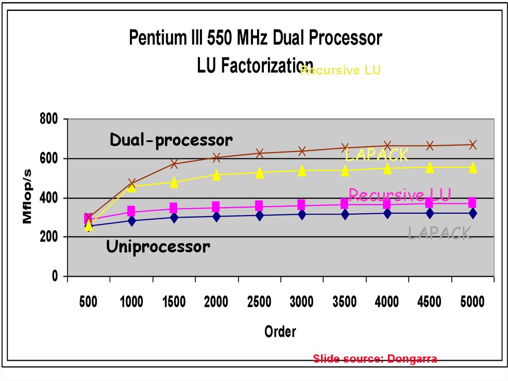
DGEMM
& DGETRF
Recursive
PentiumATLAS
III 550 MHz
Dual Processor
LU 1GHz
Factorization
AMD Athlon
(~$1100
system)
Recursive
LU
MFlop/s
Mflop/s
800
Dual-processor
400
600
300
400
200
200
100
LAPACK
Recursive LU
LAPACK
Uniprocessor
00
500
1500
500 1000 1000
2000 15002500
3000
2000 3500
4000
2500
4500 3000
5000
Order
Order
02/09/2006
CS267 Lecture 8
Slide source: Dongarra
72

72.

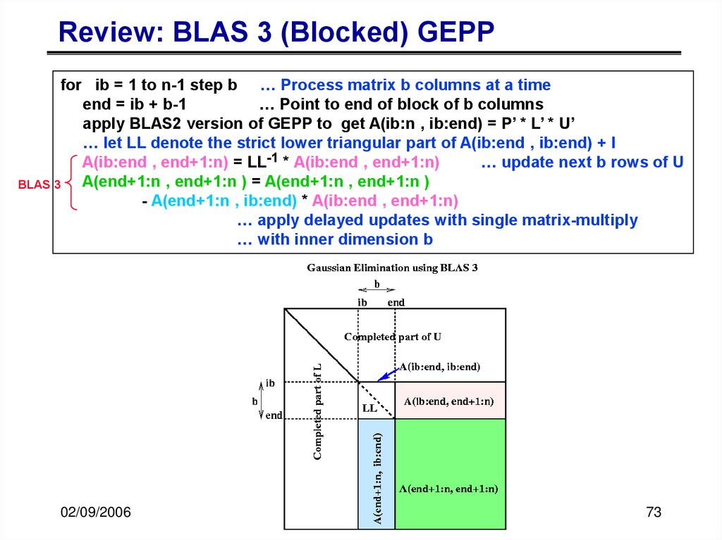
Review: BLAS 3 (Blocked) GEPP
for ib = 1 to n-1 step b … Process matrix b columns at a time
end = ib + b-1
… Point to end of block of b columns
apply BLAS2 version of GEPP to get A(ib:n , ib:end) = P’ * L’ * U’
… let LL denote the strict lower triangular part of A(ib:end , ib:end) + I
A(ib:end , end+1:n) = LL-1 * A(ib:end , end+1:n)
… update next b rows of U
A(end+1:n , end+1:n ) = A(end+1:n , end+1:n )
BLAS 3
- A(end+1:n , ib:end) * A(ib:end , end+1:n)
… apply delayed updates with single matrix-multiply
… with inner dimension b
02/09/2006
CS267 Lecture 8
73

73. Review: BLAS 3 (Blocked) GEPP

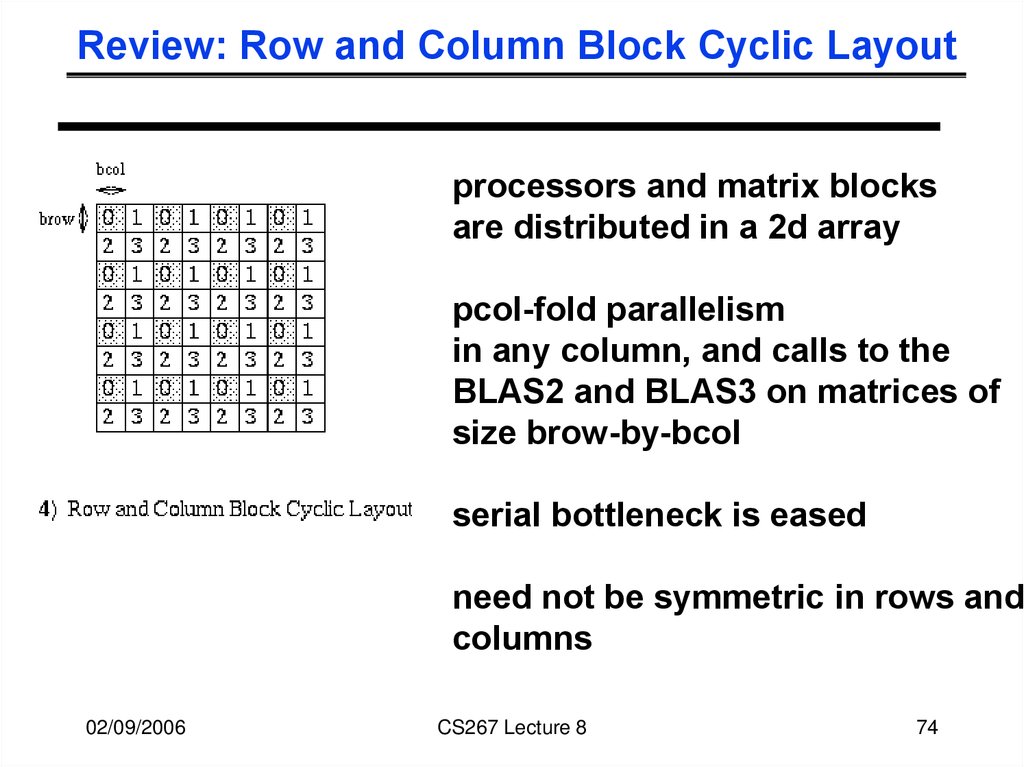
Review: Row and Column Block Cyclic Layout
processors and matrix blocks
are distributed in a 2d array
pcol-fold parallelism
in any column, and calls to the
BLAS2 and BLAS3 on matrices of
size brow-by-bcol
serial bottleneck is eased
need not be symmetric in rows and
columns
02/09/2006
CS267 Lecture 8
74

74.

Distributed GE with a 2D Block Cyclic Layout
block size b in the algorithm and the block sizes brow
and bcol in the layout satisfy b=brow=bcol.
shaded regions indicate busy processors or
communication performed.
unnecessary to have a barrier between each
step of the algorithm, e.g.. step 9, 10, and 11 can be
pipelined
02/09/2006
CS267 Lecture 8
75

75.

Distributed GE with a 2D Block Cyclic Layout
02/09/2006
CS267 Lecture 8
76

76.

02/09/2006
CS267 Lecture 8
77
green = green - blue * pink
Matrix multiply of

77.

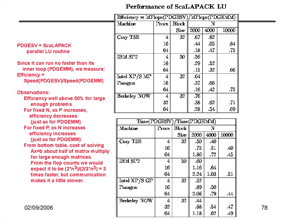
PDGESV = ScaLAPACK
parallel LU routine
Since it can run no faster than its
inner loop (PDGEMM), we measure:
Efficiency =
Speed(PDGESV)/Speed(PDGEMM)
Observations:
Efficiency well above 50% for large
enough problems
For fixed N, as P increases,
efficiency decreases
(just as for PDGEMM)
For fixed P, as N increases
efficiency increases
(just as for PDGEMM)
From bottom table, cost of solving
Ax=b about half of matrix multiply
for large enough matrices.
From the flop counts we would
expect it to be (2*n3)/(2/3*n3) = 3
times faster, but communication
makes it a little slower.
02/09/2006
CS267 Lecture 8
78

78.

02/09/2006
CS267 Lecture 8
79

79.

Scales well,
nearly full machine speed
02/09/2006
CS267 Lecture 8
80

80.

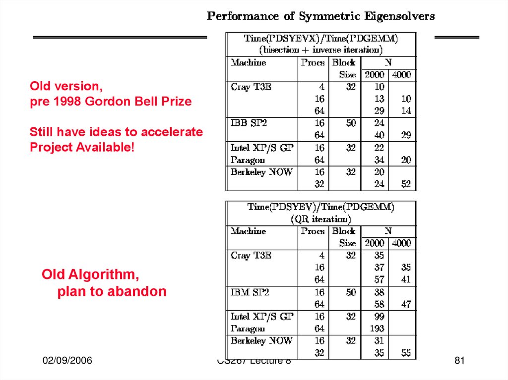
Old version,
pre 1998 Gordon Bell Prize
Still have ideas to accelerate
Project Available!
Old Algorithm,
plan to abandon
02/09/2006
CS267 Lecture 8
81

81.

Have good ideas to speedup
Project available!
Hardest of all to parallelize
Have alternative, and
would like to compare
Project available!
02/09/2006
CS267 Lecture 8
82

82.

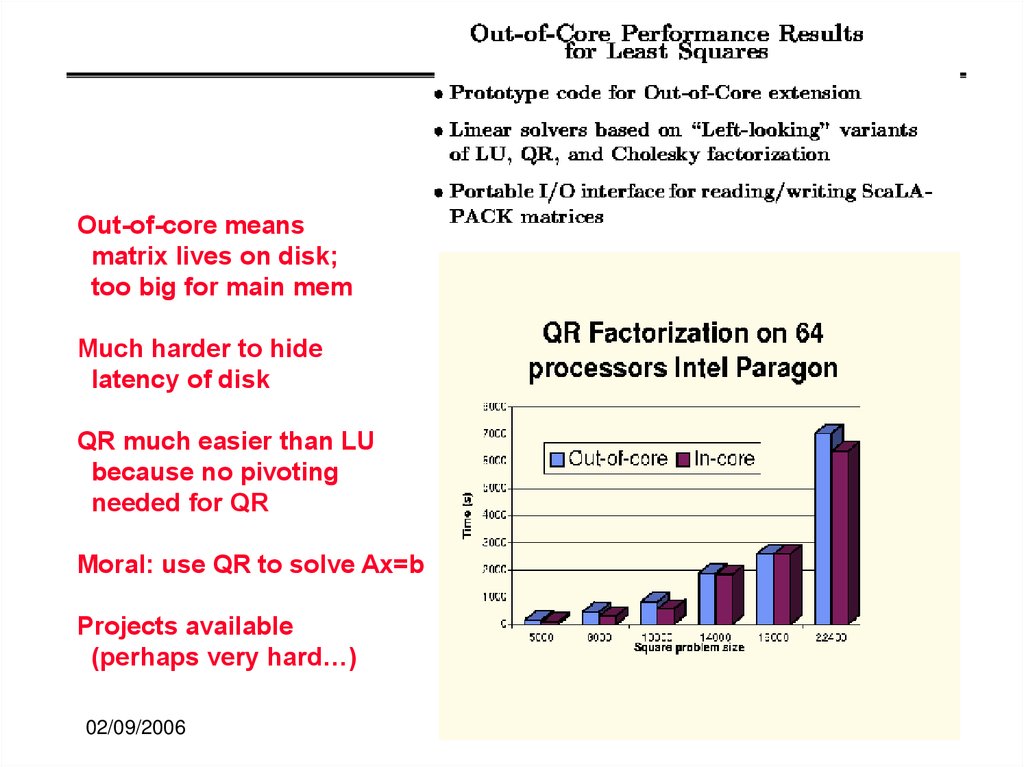
Out-of-core means
matrix lives on disk;
too big for main mem
Much harder to hide
latency of disk
QR much easier than LU
because no pivoting
needed for QR
Moral: use QR to solve Ax=b
Projects available
(perhaps very hard…)
02/09/2006
CS267 Lecture 8
83

83.

A small software project ...
02/09/2006
CS267 Lecture 8
84

84. A small software project ...

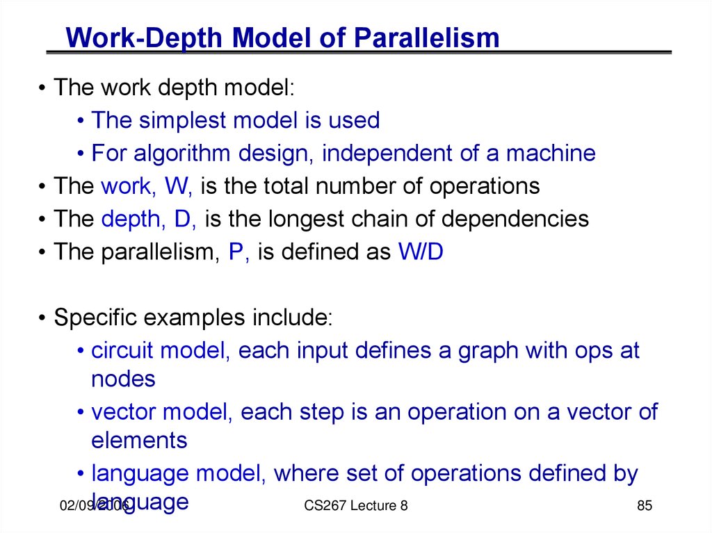
Work-Depth Model of Parallelism
• The work depth model:
• The simplest model is used
• For algorithm design, independent of a machine
• The work, W, is the total number of operations
• The depth, D, is the longest chain of dependencies
• The parallelism, P, is defined as W/D
• Specific examples include:
• circuit model, each input defines a graph with ops at
nodes
• vector model, each step is an operation on a vector of
elements
• language model, where set of operations defined by
language
02/09/2006
CS267 Lecture 8
85

85. Work-Depth Model of Parallelism

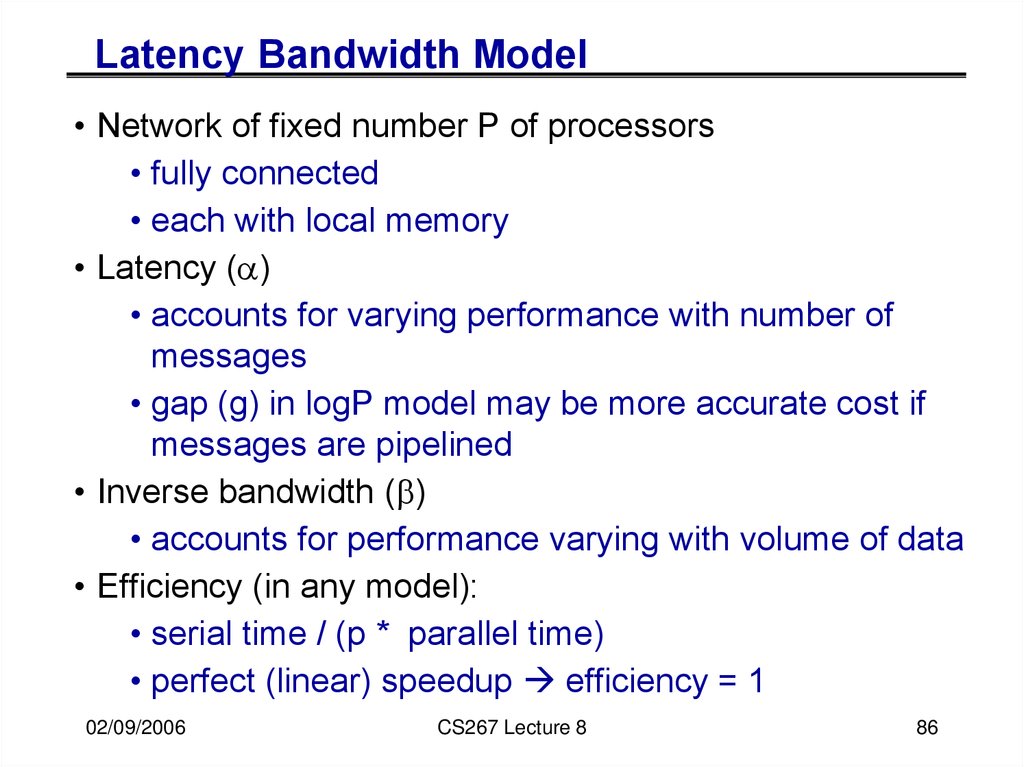
Latency Bandwidth Model
• Network of fixed number P of processors
• fully connected
• each with local memory
• Latency (a)
• accounts for varying performance with number of
messages
• gap (g) in logP model may be more accurate cost if
messages are pipelined
• Inverse bandwidth (b)
• accounts for performance varying with volume of data
• Efficiency (in any model):
• serial time / (p * parallel time)
• perfect (linear) speedup efficiency = 1
02/09/2006
CS267 Lecture 8
86

86. Latency Bandwidth Model

Initial Step to Skew Matrices in Cannon
• Initial blocked input
A(0,0) A(0,1) A(0,2)
B(0,0) B(0,1) B(0,2)
A(1,0) A(1,1) A(1,2)
B(1,0) B(1,1) B(1,2)
A(2,0) A(2,1) A(2,2)
B(2,0) B(2,1) B(2,2)
• After skewing before initial block multiplies
A(0,0) A(0,1) A(0,2)
B(0,0) B(1,1) B(2,2)
A(1,1) A(1,2) A(1,0)
B(1,0) B(2,1) B(0,2)
A(2,2) A(2,0) A(2,1)
B(2,0) B(0,1) B(1,2)
02/09/2006
CS267 Lecture 8
87

87. Initial Step to Skew Matrices in Cannon

Skewing Steps in Cannon
• First step
• Second
• Third
02/09/2006
A(0,0) A(0,1) A(0,2)
B(0,0) B(1,1) B(2,2)
A(1,1) A(1,2) A(1,0)
B(1,0) B(2,1) B(0,2)
A(2,2) A(2,0) A(2,1)
B(2,0) B(0,1) B(1,2)
A(0,1) A(0,2) A(0,0)
B(1,0) B(2,1) B(0,2)
A(1,2) A(1,0) A(1,1)
B(2,0) B(0,1) B(1,2)
A(2,0) A(2,1) A(2,2)
B(0,0) B(1,1) B(2,2)
A(0,2) A(0,0) A(0,1)
B(2,0) B(0,1) B(1,2)
A(1,0) A(1,1) A(1,2)
B(0,0) B(1,1) B(2,2)
A(2,1) A(2,2) A(2,0)
CS267 Lecture 8
B(1,0) B(2,1) B(0,2)
88

88. Skewing Steps in Cannon

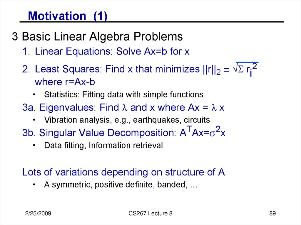
Motivation (1)
3 Basic Linear Algebra Problems
1. Linear Equations: Solve Ax=b for x
2. Least Squares: Find x that minimizes ||r||2 S ri2
where r=Ax-b
• Statistics: Fitting data with simple functions
3a. Eigenvalues: Find l and x where Ax = l x
• Vibration analysis, e.g., earthquakes, circuits
3b. Singular Value Decomposition: ATAx= 2x
• Data fitting, Information retrieval
Lots of variations depending on structure of A
• A symmetric, positive definite, banded, …
2/25/2009
CS267 Lecture 8
89

89. Motivation (1)

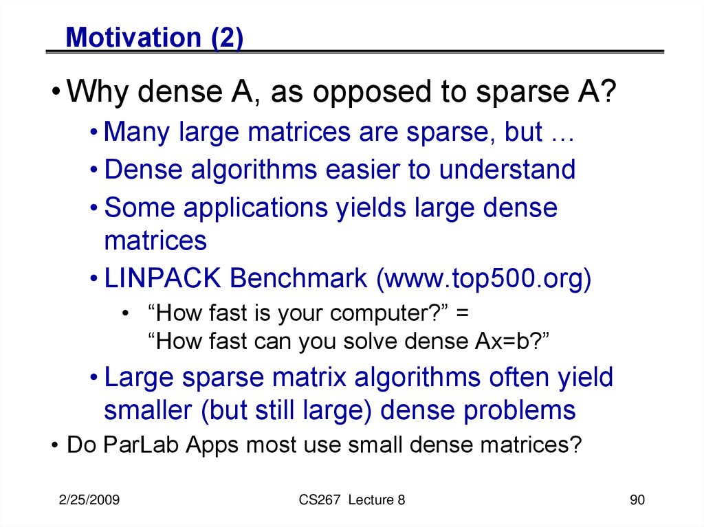
Motivation (2)
• Why dense A, as opposed to sparse A?
• Many large matrices are sparse, but …
• Dense algorithms easier to understand
• Some applications yields large dense
matrices
• LINPACK Benchmark (www.top500.org)
• “How fast is your computer?” =
“How fast can you solve dense Ax=b?”
• Large sparse matrix algorithms often yield
smaller (but still large) dense problems
• Do ParLab Apps most use small dense matrices?
2/25/2009
CS267 Lecture 8
90

90. Motivation (2)

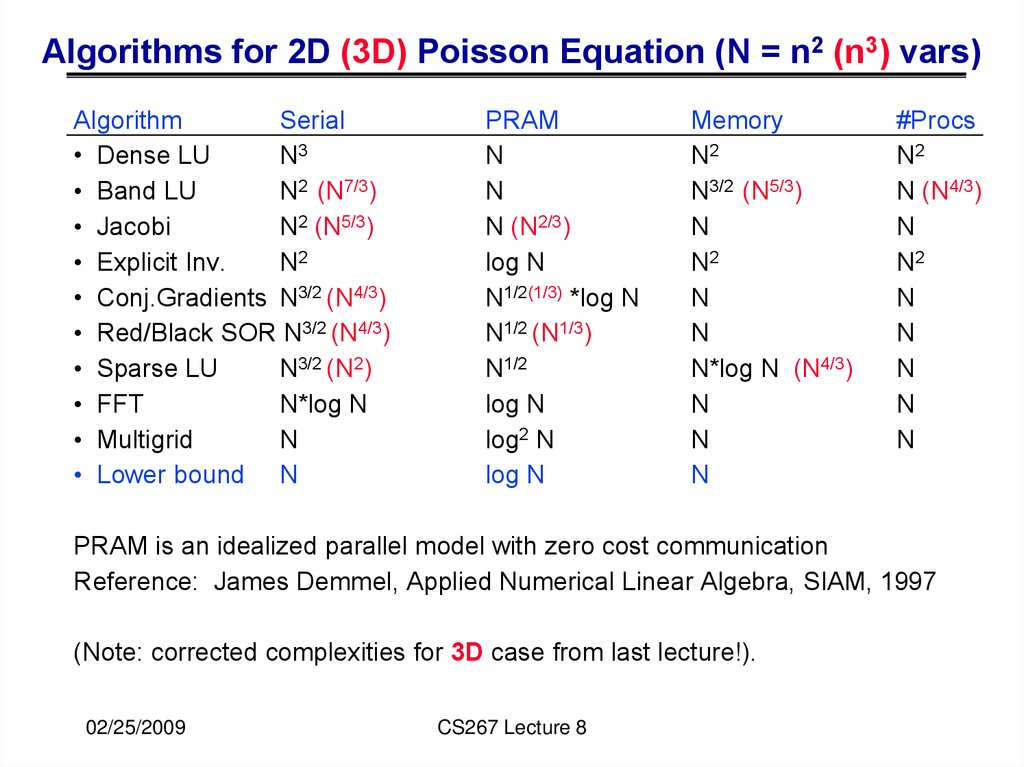
Algorithms for 2D (3D) Poisson Equation (N = n2 (n3) vars)
Algorithm
Serial
• Dense LU
N3
• Band LU
N2 (N7/3)
• Jacobi
N2 (N5/3)
• Explicit Inv.
N2
• Conj.Gradients N3/2 (N4/3)
• Red/Black SOR N3/2 (N4/3)
• Sparse LU
N3/2 (N2)
• FFT
N*log N
• Multigrid
N
• Lower bound N
PRAM
N
N
N (N2/3)
log N
N1/2(1/3) *log N
N1/2 (N1/3)
N1/2
log N
log2 N
log N
Memory
N2
N3/2 (N5/3)
N
N2
N
N
N*log N (N4/3)
N
N
N
#Procs
N2
N (N4/3)
N
N2
N
N
N
N
N
PRAM is an idealized parallel model with zero cost communication
Reference: James Demmel, Applied Numerical Linear Algebra, SIAM, 1997
(Note: corrected complexities for 3D case from last lecture!).
02/25/2009
CS267 Lecture 8

91. Algorithms for 2D (3D) Poisson Equation (N = n2 (n3) vars)

Lessons and Questions (1)
• Structure of the problem matters
• Cost of solution can vary dramatically (n3 to n)
• Many other examples
• Some structure can be figured out automatically
• “A\b” can figure out symmetry, some sparsity
• Some structures known only to (smart) user
• If performance not critical, user may be happy to settle for A\b
• How much of this goes into the motifs?
• How much should we try to help user choose?
• Tuning, but at algorithmic choice level (SALSA)
• Motifs overlap
• Dense, sparse, (un)structured grids, spectral

92. Lessons and Questions (1)

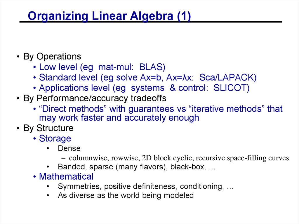
Organizing Linear Algebra (1)
• By Operations
• Low level (eg mat-mul: BLAS)
• Standard level (eg solve Ax=b, Ax=λx: Sca/LAPACK)
• Applications level (eg systems & control: SLICOT)
• By Performance/accuracy tradeoffs
• “Direct methods” with guarantees vs “iterative methods” that
may work faster and accurately enough
• By Structure
• Storage
Dense
– columnwise, rowwise, 2D block cyclic, recursive space-filling curves
Banded, sparse (many flavors), black-box, …
• Mathematical
Symmetries, positive definiteness, conditioning, …
As diverse as the world being modeled

93. Organizing Linear Algebra (1)

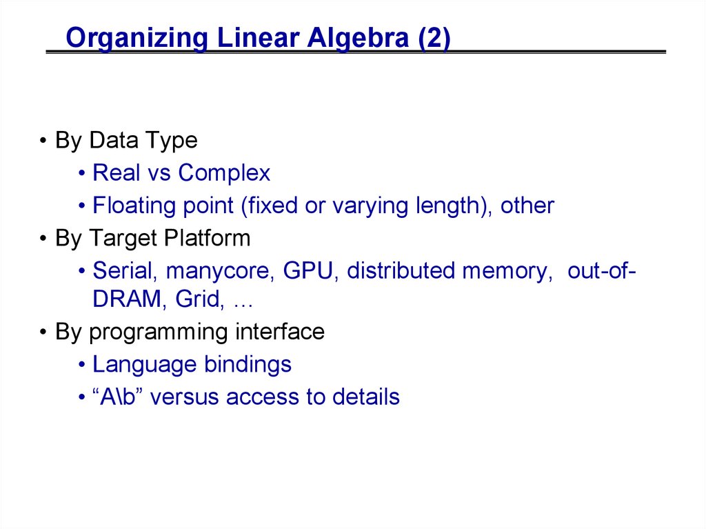
Organizing Linear Algebra (2)
• By Data Type
• Real vs Complex
• Floating point (fixed or varying length), other
• By Target Platform
• Serial, manycore, GPU, distributed memory, out-ofDRAM, Grid, …
• By programming interface
• Language bindings
• “A\b” versus access to details

94. Organizing Linear Algebra (2)

For all linear algebra problems:
Ex: LAPACK Table of Contents
• Linear Systems
• Least Squares
• Overdetermined, underdetermined
• Unconstrained, constrained, weighted
• Eigenvalues and vectors of Symmetric Matrices
Standard (Ax = λx), Generallzed (Ax=λxB)
• Eigenvalues and vectors of Unsymmetric matrices
Eigenvalues, Schur form, eigenvectors, invariant subspaces
Standard, Generalized
• Singular Values and vectors (SVD)
• Standard, Generalized
• Level of detail
• Simple Driver
• Expert Drivers with error bounds, extra-precision, other options
• Lower level routines (“apply certain kind of orthogonal transformation”)

95. For all linear algebra problems: Ex: LAPACK Table of Contents

For all matrix/problem structures:
Ex: LAPACK Table of Contents
BD – bidiagonal
GB – general banded
GE – general
GG – general , pair
GT – tridiagonal
HB – Hermitian banded
HE – Hermitian
HG – upper Hessenberg, pair
HP – Hermitian, packed
HS – upper Hessenberg
OR – (real) orthogonal
OP – (real) orthogonal, packed
PB – positive definite, banded
PO – positive definite
PP – positive definite, packed
PT – positive definite, tridiagonal
SB – symmetric, banded
SP – symmetric, packed
ST – symmetric, tridiagonal
SY – symmetric
TB – triangular, banded
TG – triangular, pair
TB – triangular, banded
TP – triangular, packed
TR – triangular
TZ – trapezoidal
UN – unitary
UP – unitary packed

96. For all matrix/problem structures: Ex: LAPACK Table of Contents

BD – bidiagonal
GB – general banded
GE – general
GG – general , pair
GT – tridiagonal
HB – Hermitian banded
HE – Hermitian
HG – upper Hessenberg, pair
HP – Hermitian, packed
HS – upper Hessenberg
OR – (real) orthogonal
OP – (real) orthogonal, packed
PB – positive definite, banded
PO – positive definite
PP – positive definite, packed
PT – positive definite, tridiagonal
SB – symmetric, banded
SP – symmetric, packed
ST – symmetric, tridiagonal
SY – symmetric
TB – triangular, banded
TG – triangular, pair
TB – triangular, banded
TP – triangular, packed
TR – triangular
TZ – trapezoidal
UN – unitary
UP – unitary packed

97. For all matrix/problem structures: Ex: LAPACK Table of Contents

BD – bidiagonal
GB – general banded
GE – general
GG – general, pair
GT – tridiagonal
HB – Hermitian banded
HE – Hermitian
HG – upper Hessenberg, pair
HP – Hermitian, packed
HS – upper Hessenberg
OR – (real) orthogonal
OP – (real) orthogonal, packed
PB – positive definite, banded
PO – positive definite
PP – positive definite, packed
PT – positive definite, tridiagonal
SB – symmetric, banded
SP – symmetric, packed
ST – symmetric, tridiagonal
SY – symmetric
TB – triangular, banded
TG – triangular, pair
TB – triangular, banded
TP – triangular, packed
TR – triangular
TZ – trapezoidal
UN – unitary
UP – unitary packed

98. For all matrix/problem structures: Ex: LAPACK Table of Contents

BD – bidiagonal
GB – general banded
GE – general
GG – general, pair
GT – tridiagonal
HB – Hermitian banded
HE – Hermitian
HG – upper Hessenberg, pair
HP – Hermitian, packed
HS – upper Hessenberg
OR – (real) orthogonal
OP – (real) orthogonal, packed
PB – positive definite, banded
PO – positive definite
PP – positive definite, packed
PT – positive definite, tridiagonal
SB – symmetric, banded
SP – symmetric, packed
ST – symmetric, tridiagonal
SY – symmetric
TB – triangular, banded
TG – triangular, pair
TB – triangular, banded
TP – triangular, packed
TR – triangular
TZ – trapezoidal
UN – unitary
UP – unitary packed

99. For all matrix/problem structures: Ex: LAPACK Table of Contents

BD – bidiagonal
GB – general banded
GE – general
GG – general, pair
GT – tridiagonal
HB – Hermitian banded
HE – Hermitian
HG – upper Hessenberg, pair
HP – Hermitian, packed
HS – upper Hessenberg
OR – (real) orthogonal
OP – (real) orthogonal, packed
PB – positive definite, banded
PO – positive definite
PP – positive definite, packed
PT – positive definite, tridiagonal
SB – symmetric, banded
SP – symmetric, packed
ST – symmetric, tridiagonal
SY – symmetric
TB – triangular, banded
TG – triangular, pair
TB – triangular, banded
TP – triangular, packed
TR – triangular
TZ – trapezoidal
UN – unitary
UP – unitary packed

100. For all matrix/problem structures: Ex: LAPACK Table of Contents

BD – bidiagonal
GB – general banded
GE – general
GG – general , pair
GT – tridiagonal
HB – Hermitian banded
HE – Hermitian
HG – upper Hessenberg, pair
HP – Hermitian, packed
HS – upper Hessenberg
OR – (real) orthogonal
OP – (real) orthogonal, packed
PB – positive definite, banded
PO – positive definite
PP – positive definite, packed
PT – positive definite, tridiagonal
SB – symmetric, banded
SP – symmetric, packed
ST – symmetric, tridiagonal
SY – symmetric
TB – triangular, banded
TG – triangular, pair
TB – triangular, banded
TP – triangular, packed
TR – triangular
TZ – trapezoidal
UN – unitary
UP – unitary packed

101. For all matrix/problem structures: Ex: LAPACK Table of Contents

BD – bidiagonal
GB – general banded
GE – general
GG – general, pair
GT – tridiagonal
HB – Hermitian banded
HE – Hermitian
HG – upper Hessenberg, pair
HP – Hermitian, packed
HS – upper Hessenberg
OR – (real) orthogonal
OP – (real) orthogonal, packed
PB – positive definite, banded
PO – positive definite
PP – positive definite, packed
PT – positive definite, tridiagonal
SB – symmetric, banded
SP – symmetric, packed
ST – symmetric, tridiagonal
SY – symmetric
TB – triangular, banded
TG – triangular, pair
TB – triangular, banded
TP – triangular, packed
TR – triangular
TZ – trapezoidal
UN – unitary
UP – unitary packed

102. For all matrix/problem structures: Ex: LAPACK Table of Contents

For all data types:
Ex: LAPACK Table of Contents
• Real and complex
• Single and double precision
• Arbitrary precision in progress

103. For all data types: Ex: LAPACK Table of Contents

Organizing Linear Algebra (3)
www.netlib.org/lapack
www.netlib.org/scalapack
gams.nist.gov
www.netlib.org/templates
www.cs.utk.edu/~dongarra/etemplates

104. Organizing Linear Algebra (3)

Review of the BLAS
• Building blocks for all linear algebra
• Parallel versions call serial versions on each processor
• So they must be fast!
• Define q = # flops / # mem refs = “computational intensity”
• The larger is q, the faster the algorithm can go in the
presence of memory hierarchy
• “axpy”: y = a*x + y, where a scalar, x and y vectors
BLAS level
Ex.
# mem refs
# flops
q
1
“Axpy”,
Dot prod
3n
2n1
2/3
2
Matrixvector mult
n2
2n2
2
3
Matrixmatrix mult
4n2
2n3
n/2
2/27/08
CS267 Guest Lecture 1
105