
 mathematics
Similar presentations:


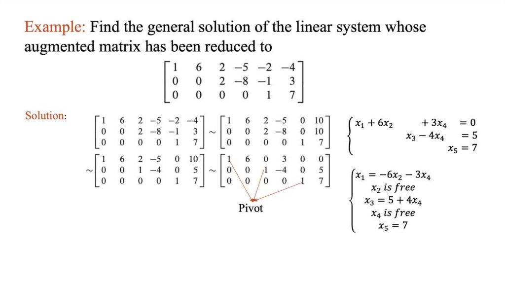
Linear Equations in Linear Algebra
1.
Lecture 1Linear Equations in Linear Algebra
1.1 Systems of Linear Equations;
1.2 Row Reduction and Echelon Forms;
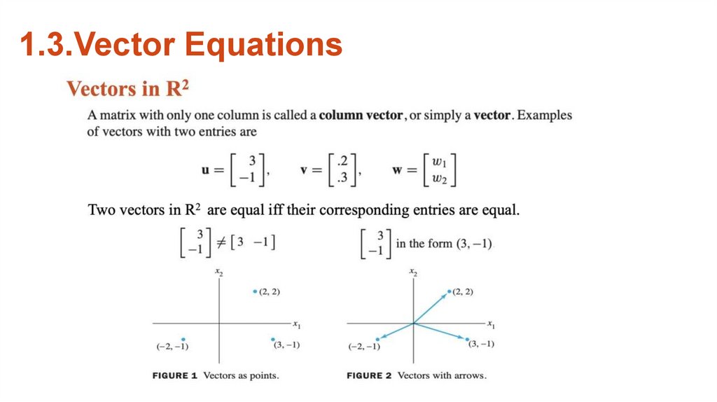
1.3 Vector Equations;
1.4 The Matrix Equation;
1.5 Solution Sets of Linear Systems
2.
Learning Objectives:1. Represent a system of linear equations as an augmented
matrix.
2. Identify whether the matrix is in row-echelon form, reduced
row-echelon form, both, or neither.
3. Solve systems of linear equations.
4. Consider vectors in R2 and R3.
5. Compute Ax.
6. Perform matrix operations of addition, subtraction,
multiplication, and multiplication by a scalar.
3.
1.1. Systems of Linear EquationsA linear equation in two variables can be written in the form ax + by =
k, where a, b, and k are constants, and a and b are coefficients not
equal to 0.
Note: The power of the variables is always 1.
Two or more linear equations is called a system of linear equations
because they involve solving more than one linear equation at once.
A system of linear equations can have either exactly one solution
(unique), no solution, or infinitely many solutions.
The set of all possible solutions is called the solution set of the linear
system. Two linear systems are called equivalent if they have the same
solution set.
4.
Possible graphs of a System of Two LinearEquations in two variables.
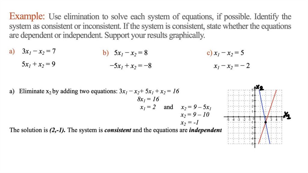
1.The graphs of the two equations are distinct line that intersect at one
point. The system is consistent. There is one solution, which is given
by the coordinates of the point of intersection. In this case the
equations are independent.
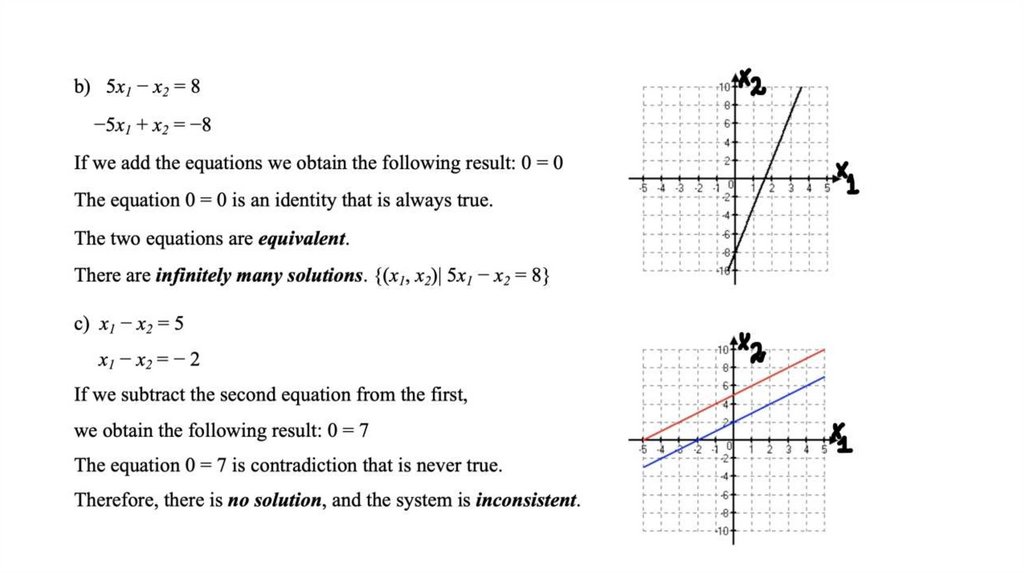
2.The graphs of the two equations are the same line. The system is
consistent. There are infinitely many solutions, and the equations are
dependent.
3.The graphs of the two equations are distinct parallel lines. The system
is inconsistent. There are no solutions.
5.
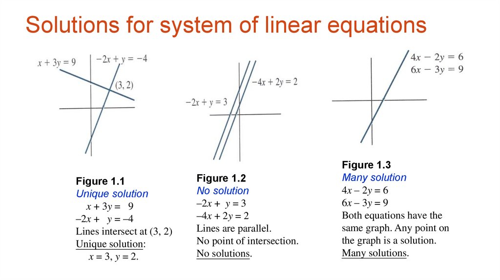
Solutions for system of linear equationsFigure 1.1
Unique solution
x + 3y = 9
–2x + y = –4
Lines intersect at (3, 2)
Unique solution:
x = 3, y = 2.
Figure 1.2
No solution
–2x + y = 3
–4x + 2y = 2
Lines are parallel.
No point of intersection.
No solutions.
Figure 1.3
Many solution
4x – 2y = 6
6x – 3y = 9
Both equations have the
same graph. Any point on
the graph is a solution.
Many solutions.
6.
7.
8.
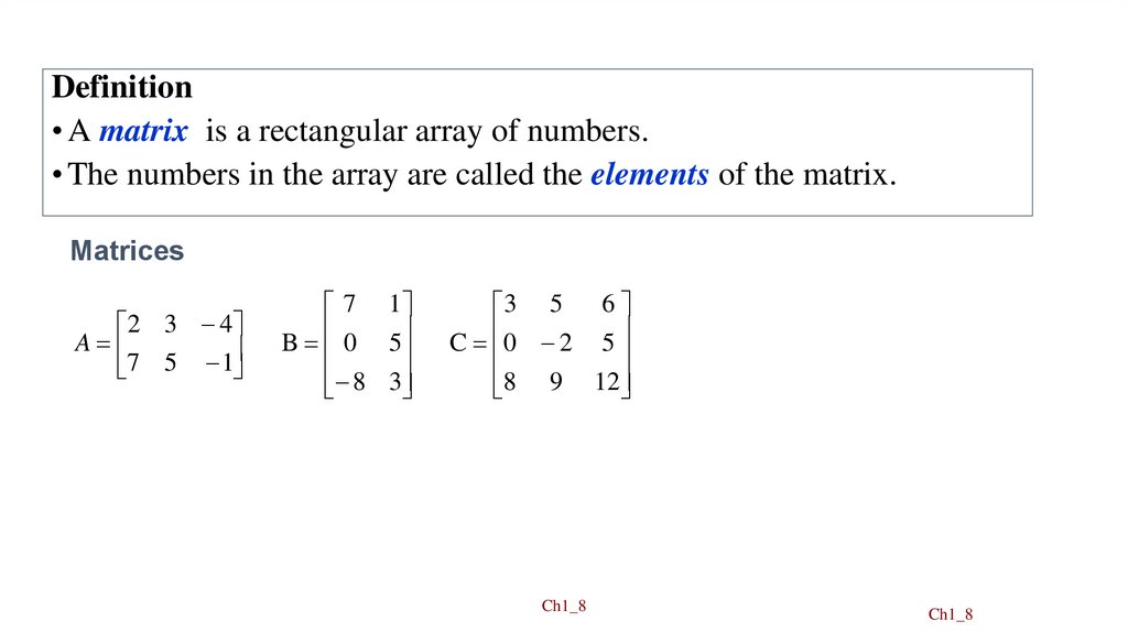
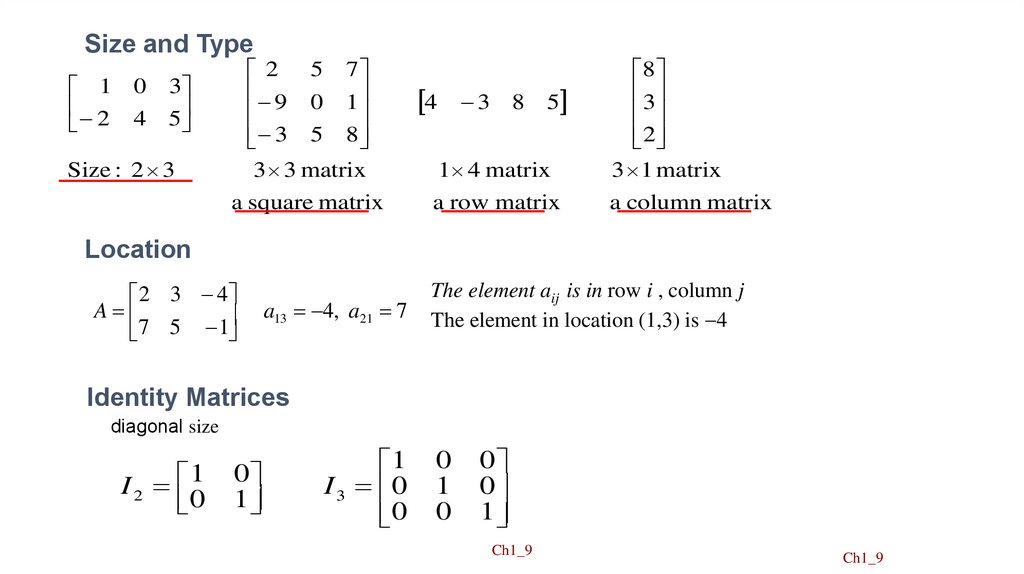
Definition• A matrix is a rectangular array of numbers.
• The numbers in the array are called the elements of the matrix.
Matrices
2 3 4
A
7
5
1
7 1
B 0 5
8 3
3 5 6
C 0 2 5
8 9 12
Ch1_8
Ch1_8
9.
Size and Type1 0
2 4
3
5
Size : 2 3
2 5 7
9 0 1
3 5 8
3 3 matrix
a square matrix
4
3 8
5
1 4 matrix
a row matrix
8
3
2
3 1 matrix
a column matrix
Location
2 3 4
A
7 5 1
a13 4, a21 7
The element aij is in row i , column j
The element in location (1,3) is 4
Identity Matrices
diagonal size
I 2 1
0
0
1
1
I 3 0
0
0
1
0
0
0
1
Ch1_9
Ch1_9
10.
2 3 4A
7
5
1
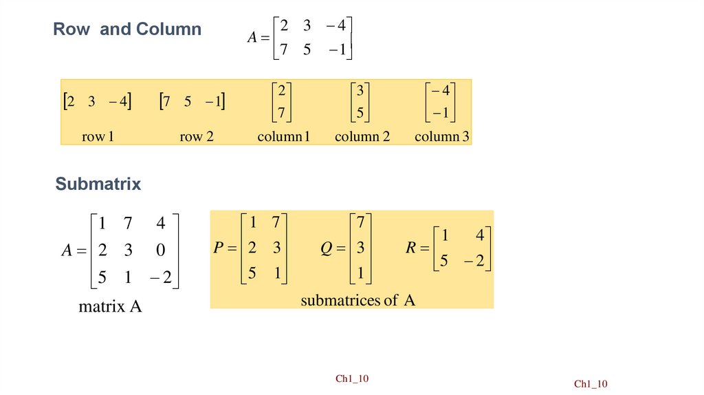
Row and Column
2 3 4
7 5 1
row 1
row 2
2
7
column 1
3
5
column 2
4
1
column 3
Submatrix
1 7 4
A 2 3 0
5 1 2
matrix A
1 7
P 2 3
5 1
7
4
1
Q 3
R
5
2
1
submatrices of A
Ch1_10
Ch1_10
11.
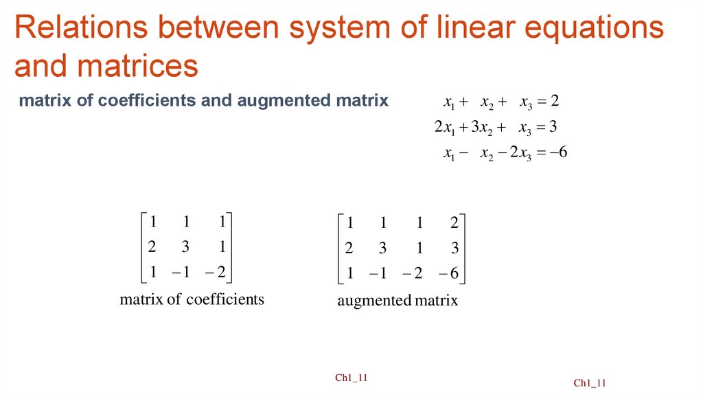
Relations between system of linear equationsand matrices
matrix of coefficients and augmented matrix
x1 x2 x3 2
2 x1 3x2 x3 3
x1 x2 2 x3 6
1
1 1
2 3
1
1 1 2
matrix of coefficients
1
2
1 1
2 3
1
3
1 1 2 6
augmented matrix
Ch1_11
Ch1_11
12.
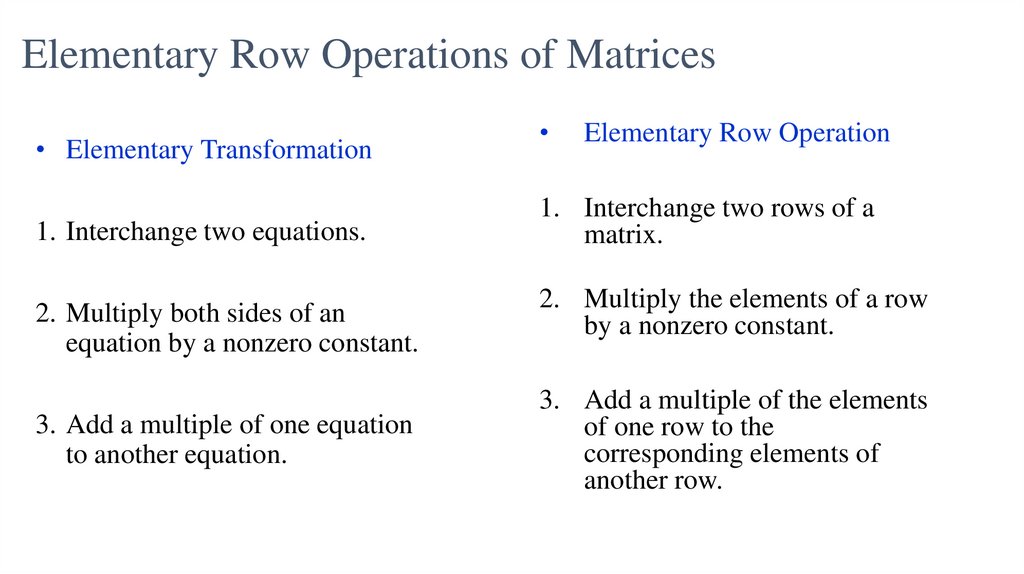
Elementary Row Operations of Matrices• Elementary Transformation
1. Interchange two equations.
2. Multiply both sides of an
equation by a nonzero constant.
3. Add a multiple of one equation
to another equation.
Elementary Row Operation
1. Interchange two rows of a
matrix.
2. Multiply the elements of a row
by a nonzero constant.
3. Add a multiple of the elements
of one row to the
corresponding elements of
another row.
13.
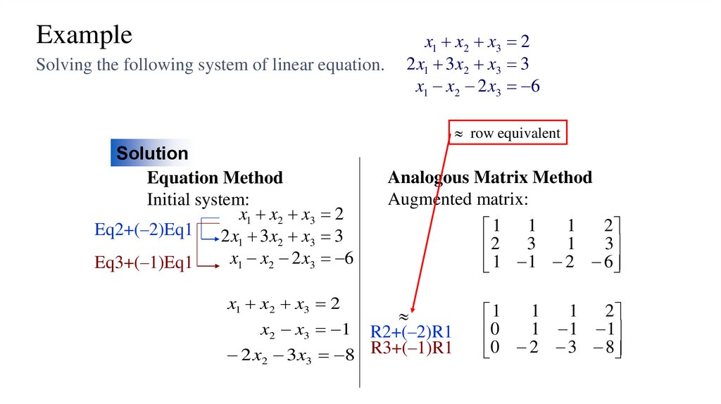
ExampleSolving the following system of linear equation.
x1 x2 x3 2
2 x1 3 x2 x3 3
x1 x2 2 x3 6
row equivalent
Solution
Equation Method
Initial system:
x1 x2 x3 2
Eq2+(–2)Eq1
2 x1 3 x2 x3 3
x1 x2 2 x3 6
Eq3+(–1)Eq1
x1 x2 x3 2
Analogous Matrix Method
Augmented matrix:
1
2
1 1
1
3
2 3
1 1 2 6
x2 x3 1 R2+(–2)R1
2 x2 3 x3 8 R3+(–1)R1
1
1
2
1
1 1 1
0
0 2 3 8
14.
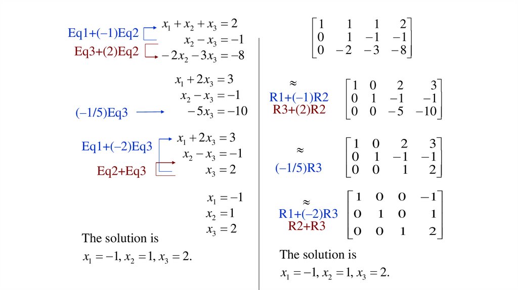
Eq1+(–1)Eq2Eq3+(2)Eq2
x1 x2 x3 2
x2 x3 1
2 x2 3 x3 8
(–1/5)Eq3
x1 2 x3 3
x2 x3 1
5 x3 10
R1+(–1)R2
R3+(2)R2
2
3
1 0
0 1 1 1
0 0 5 10
x1 2 x3 3
x2 x3 1
x3 2
(–1/5)R3
2
3
1 0
0 1 1 1
1
2
0 0
R1+(–2)R3
R2+R3
1
0
0
Eq1+(–2)Eq3
Eq2+Eq3
The solution is
x1 1, x2 1, x3 2.
x1 1
x2 1
x3 2
1
1
2
1
1 1 1
0
0 2 3 8
0
1
0
The solution is
x1 1, x2 1, x3 2.
0
0
1
1
1
2
15.
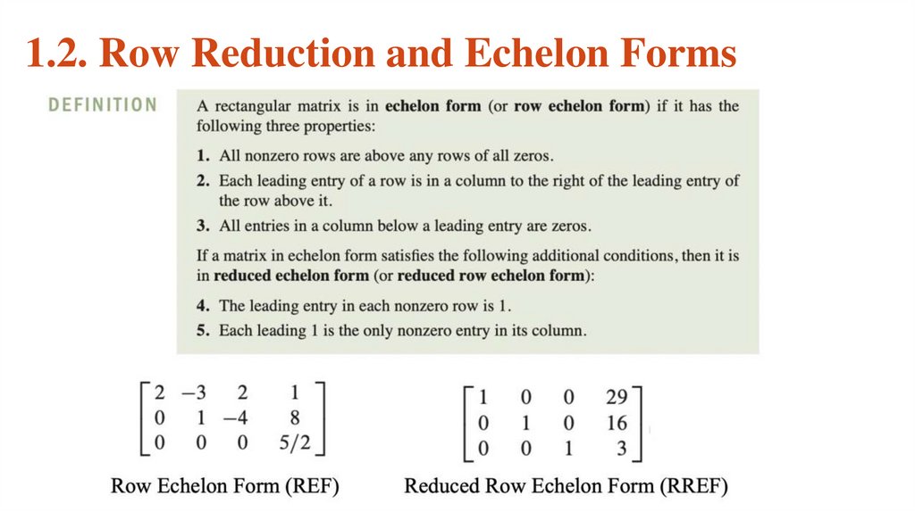
1.2. Row Reduction and Echelon Forms16.
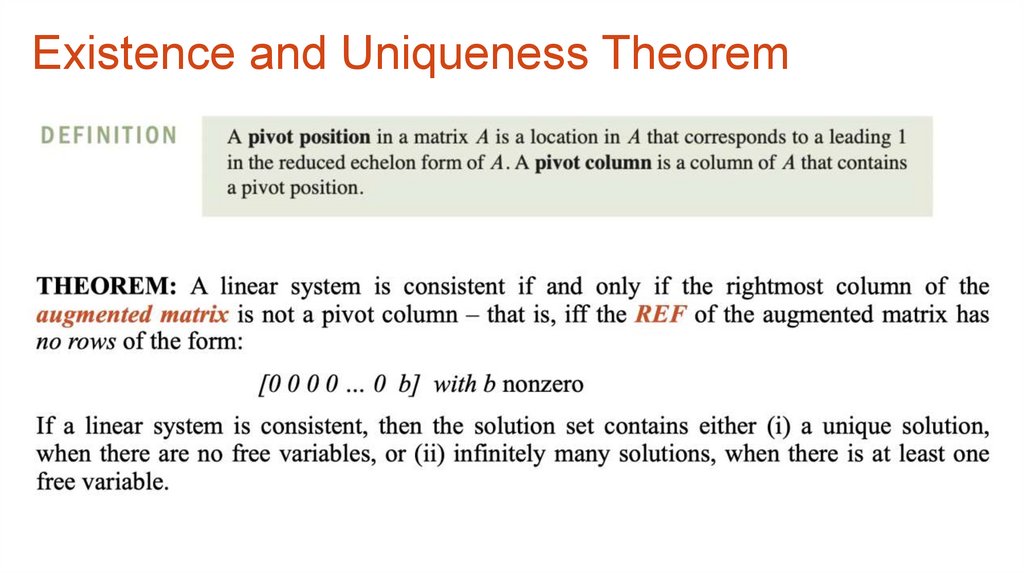
Existence and Uniqueness Theorem17.
18.
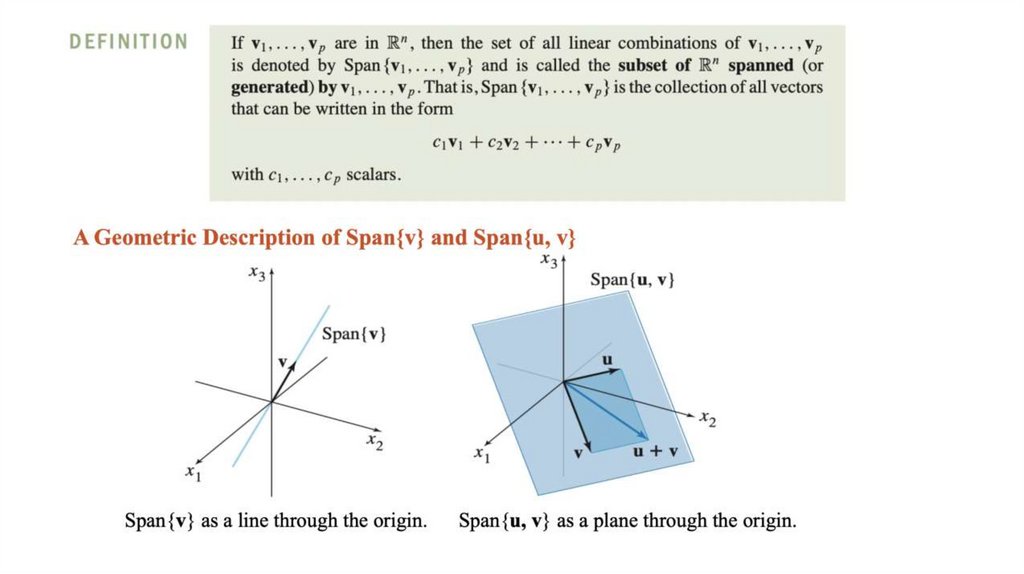
1.3.Vector Equations19.
20.
21.
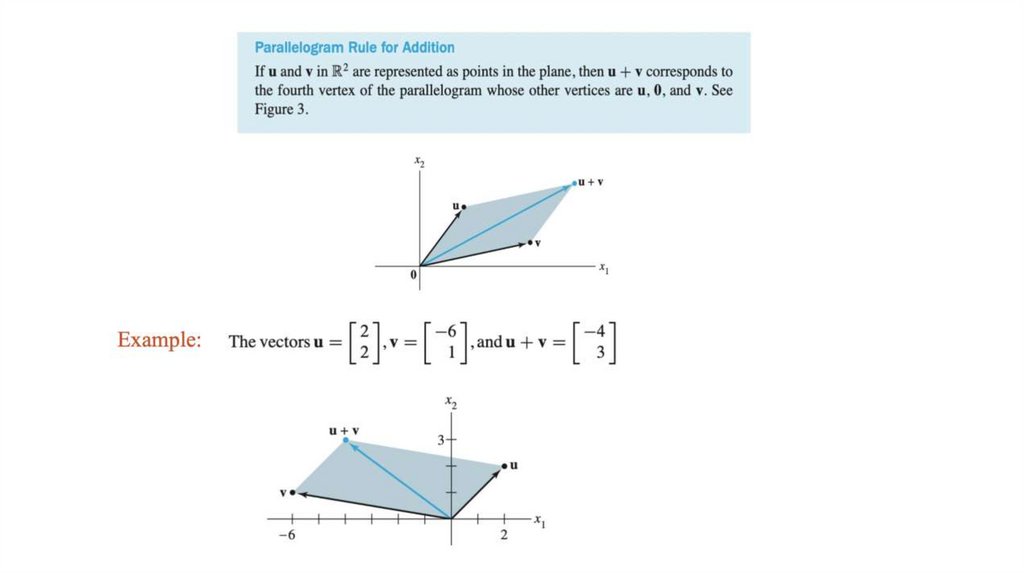
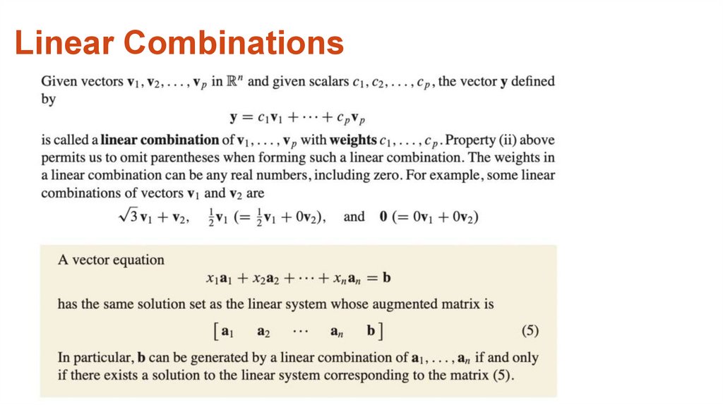
Linear Combinations22.
23.
24.
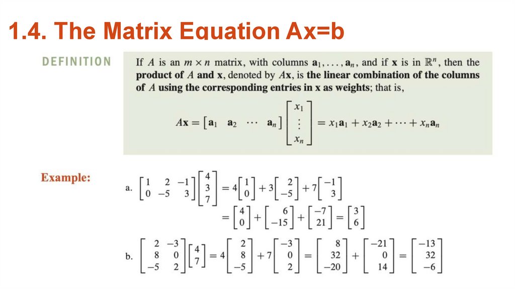
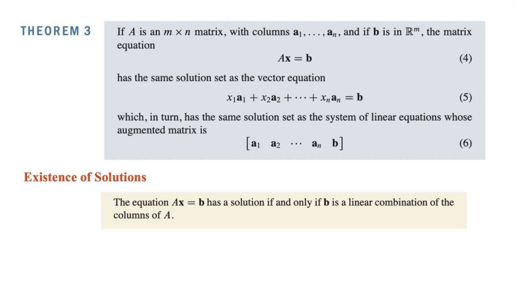
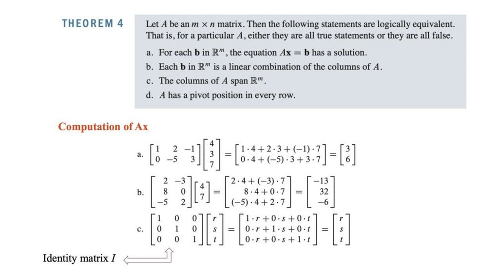
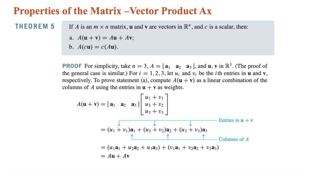
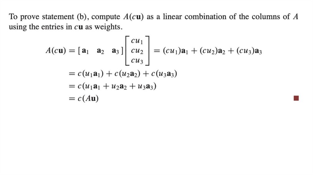
1.4. The Matrix Equation Ax=b25.
26.
27.
28.
29.
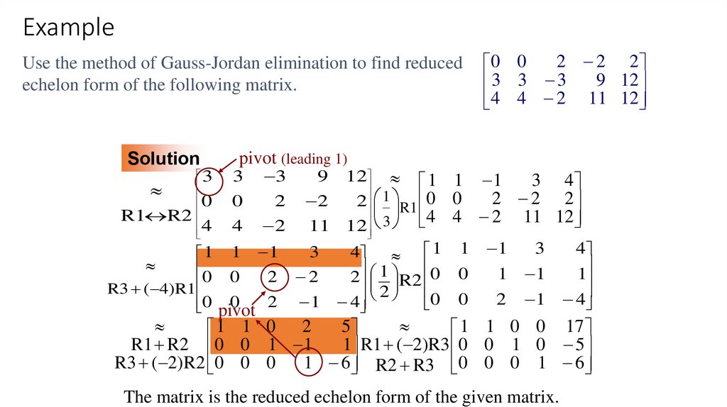
ExampleUse the method of Gauss-Jordan elimination to find reduced
echelon form of the following matrix.
Solution
pivot (leading 1)
3
0
R1 R2
4
3
0
4
3
2
2
1 1 1
2
0 0
R3 ( 4)R1
0 0
pivot 2
2 2 2
0 0
9 12
3 3 3
4 4 2 11 12
9 12 1 1 1
3 4
2 2 2
2
2 1 R1 0 0
4 4 2 11 12
11 12 3
3
4
1 1 1
3
4
1
1 1
1
2
2 R2 0 0
2
0
0
2
1
4
1 4
5
1 1 0 0 17
1 1 0 2
R1 R2 0 0 1 1
1 R1 ( 2)R3 0 0 1 0 5
R3 ( 2)R2 0 0 0
1 6 R2 R3 0 0 0 1 6
The matrix is the reduced echelon form of the given matrix.
30.
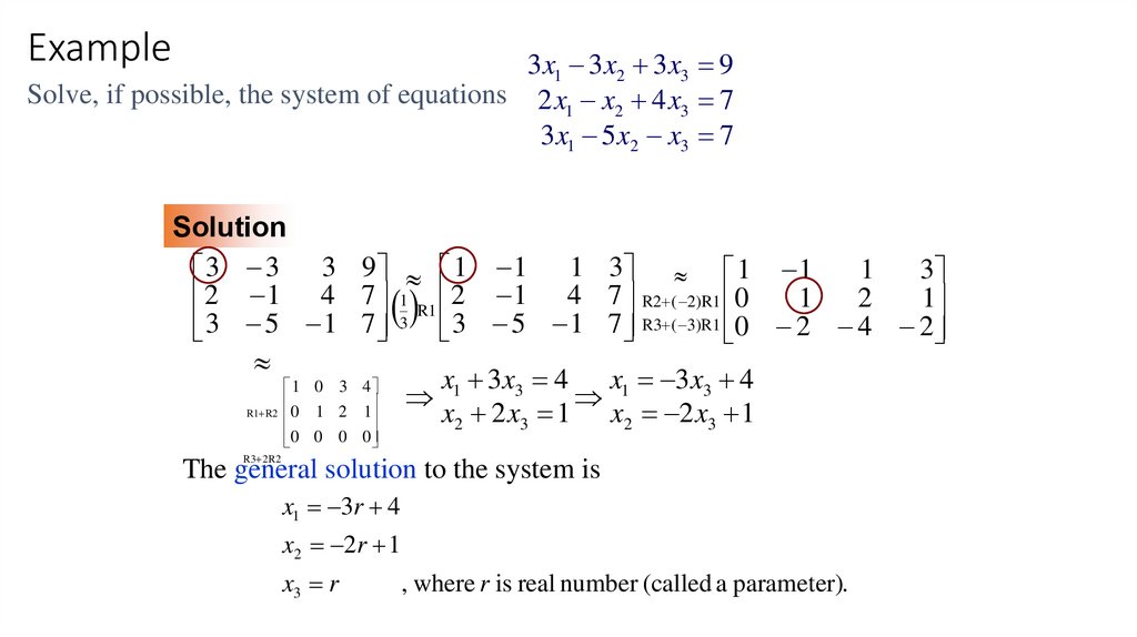
Example3 x1 3 x2 3 x3 9
Solve, if possible, the system of equations 2 x1 x2 4 x3 7
3 x1 5 x2 x3 7
Solution
1
3
3 3 3 9 1 1 1 3 1 1
1
2
1
2 1 4 7 1 R1 2 1 4 7 R2 ( 2)R1 0
3 5 1 7 3 3 5 1 7 R3 ( 3)R1 0 2 4 2
1 0 3 4
R1 R2 0
1 2 1
0 0 0 0
x 3 x3 4 x1 3 x3 4
1
x2 2 x3 1 x2 2 x3 1
R3 2R2
The general solution to the system is
x1 3r 4
x2 2r 1
x3 r
, where r is real number (called a parameter).
31.
ExampleSolve the system of equations
Solution
2 4 12
2 3
1
9
2 4
1 2
R2 R1 0
0
R3 ( 2)R1
0
0
1 2
R1 ( 6)R2 0
0
R3 3R2
0
0
2 x1 4 x2 12 x3 10 x4 58
x1 2 x2 3 x3 2 x4 14
2 x1 4 x2 9 x3 6 x4 44
many sol.
10
58 1 2
6 5
29
2 14 1 R1 1
2 3
2 14
6
44 2 2 4
9 6
44
6 5
29 1 2
6 5
29
3 3
15 1 R2 0
0
1 1
5
3
4 14 3 0
0 3
4 14
0
1 1 1 2 0 0 2
1 1 5 R1 ( 1)R3 0
0 1 0
6
0
1 1 R2 R3 0
0 0 1
1
x1 2r 2
x1 2 x2 2
x2 r
x3 6
, for some r.
x3 6
x4 1Ch1_31
x4 1
Ch1_31
32.
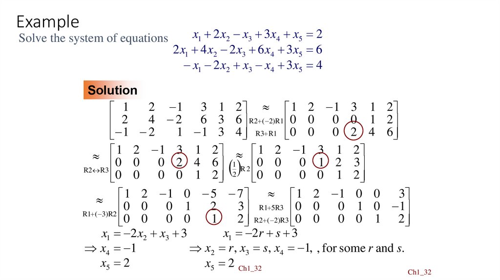
ExampleSolve the system of equations
x1 2 x2 x3 3 x4 x5 2
2 x1 4 x2 2 x3 6 x4 3 x5 6
x1 2 x2 x3 x4 3 x5 4
Solution
2 1 3 1 2 1 2 1 3 1 2
1
4 2 6 3 6 R2 ( 2)R1 0 0 0 0 1 2
2
1 1 3 4 R3 R1 0 0 0 2 4 6
1 2
1 2 1 3 1 2 1 2 1 3 1 2
0 0 0 2 4 6
0 0 0 1 2 3
1
R
2
R2 R3
0 0 0 0 1 2 2 0 0 0 0 1 2
1 2 1 0 5 7
1 2 1 0 0 3
0 0 0 1
2
3 R1 5R3 0 0 0 1 0 1
R1 ( 3)R2
1
2 R2 ( 2)R3 0 0 0 0 1 2
0 0 0 0
x1 2r s 3
x1 2 x2 x3 3
x4 1
x2 r , x3 s, x4 1, , for some r and s.
x5 2
x5 2 Ch1_32
Ch1_32
33.
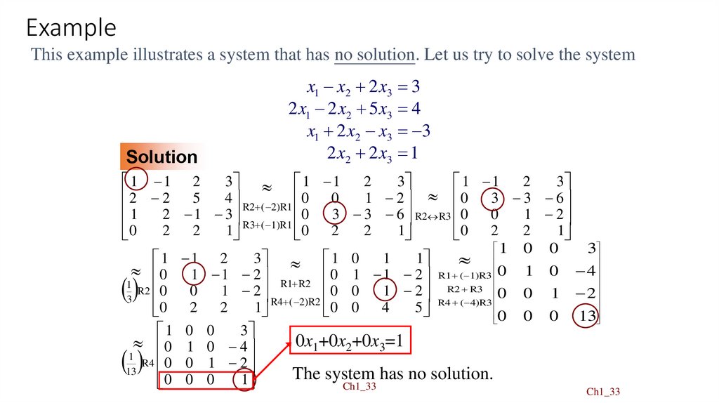
ExampleThis example illustrates a system that has no solution. Let us try to solve the system
x1 x2 2 x3 3
2 x1 2 x2 5 x3 4
x1 2 x2 x3 3
2 x2 2 x3 1
Solution
1 1 2 3 1 1 2 3
1 1 2 3
2 2 5 4 R2 ( 2)R1 0 0 1 2 0 3 3 6
1 2 1 3 R3 ( 1)R1 0 3 3 6 R2 R3 0 0 1 2
0 2 2 1
0 2 2 1
0 2 2 1
1
0 0
3
1 1 2 3 1 0 1 1
0
1
0
4
0 1 1 2
0 1 1 2 R1 ( 1)R3
R1
R2
1
R2
R3
R2
0
0
1
2
0
0
1
2
3
R4 ( 2)R2
R4 ( 4)R3 0 0 1 2
0 2 2 1
0 0 4 5
0
0 0 13
1 0 0 3
0x1+0x2+0x3=1
0 1 0 4
131 R4 0 0 1 2 The system has no solution.
0 0 0 1
Ch1_33
Ch1_33