Similar presentations:
Matlab Linear Programming
1. MATLAB Linear Programming
Greg Reese, Ph.DResearch Computing Support Group
Academic Technology Services
Miami University
2. MATLAB Linear Programming
© 2010-2013 Greg Reese. All rights reserved2
3. Optimization
Optimization - finding value of a parameterthat maximizes or minimizes a function with
that parameter
– Talking about mathematical optimization, not
optimization of computer code!
– "function" is mathematical function, not
MATLAB language function
3
4. Optimization
Optimization– Can have multiple parameters
– Can have multiple functions
– Parameters can appear linearly or
nonlinearly
4
5. Linear programming
Linear programming• Most often used kind of optimization
• Tremendous number of practical
applications
• "Programming" means determining
feasible programs (plans, schedules,
allocations) that are optimal with
respect to a certain criterion and that
obey certain constraints
5
6. Linear programming
A feasible program is a solution to alinear programming problem and that
satisfies certain constraints
In linear programming
• Constraints are linear inequalities
• Criterion is a linear expression
– Expression called the objective function
– In practice, objective function is often
the cost of or profit from some activity
6
7. Linear programming
Many important problems ineconomics and management can be
solved by linear programming
Some problems are so common that
they're given special names
7
8. Linear programming
DIET PROBLEMYou are given a group of foods, their
nutritional values and costs. You know how
much nutrition a person needs.
What combination of foods can you serve
that meets the nutritional needs of a person
but costs the least?
8
9. Linear programming
BLENDING PROBLEM–Closely relate to diet problem
Given quantities and qualities of available
oils, what is cheapest way to blend them
into needed assortment of fuels?
9
10. Linear programming
TRANSPORTATION PROBLEMYou are given a group of ports or supply centers of
a certain commodity and another group of
destinations or markets to which commodity must
be shipped. You know how much commodity at
each port, how much each market must receive,
cost to ship between any port and market.
How much should you ship from each port to each
market so as to minimize the total shipping cost?
10
11. Linear programming
WAREHOUSE PROBLEMYou are given a warehouse of known capacity and
initial stock size. Know purchase and selling price
of stock. Interested in transactions over a certain
time, e.g., year. Divide time into smaller periods,
e.g., months.
How much should you buy and sell each period to
maximize your profit, subject to restrictions that
1. Amount of stock at any time can't exceed warehouse
capacity
2. You can't sell more stock than you have
11
12. Linear programming
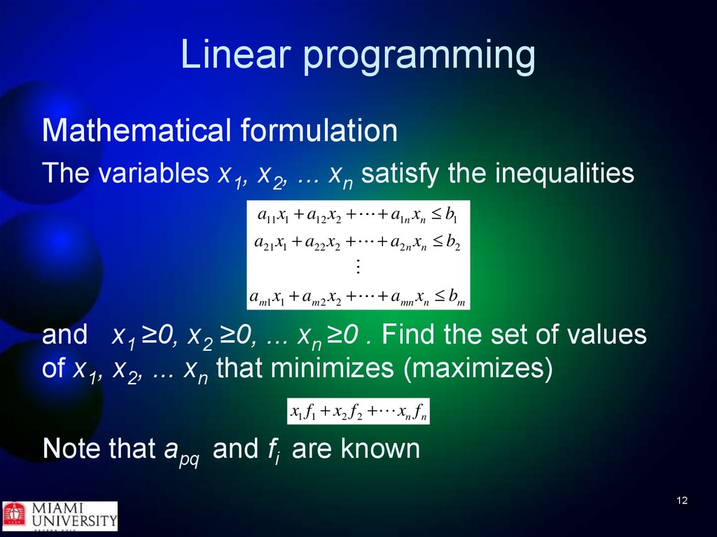
Mathematical formulationThe variables x1, x2, ... xn satisfy the inequalities
a11 x1 a12 x2 a1n xn b1
a21x1 a22 x2 a2 n xn b2
am1 x1 am 2 x2 amn xn bm
and x1 ≥0, x2 ≥0, ... xn ≥0 . Find the set of values
of x1, x2, ... xn that minimizes (maximizes)
x1 f1 x2 f 2 xn f n
Note that apq and fi are known
12
13. Linear programming
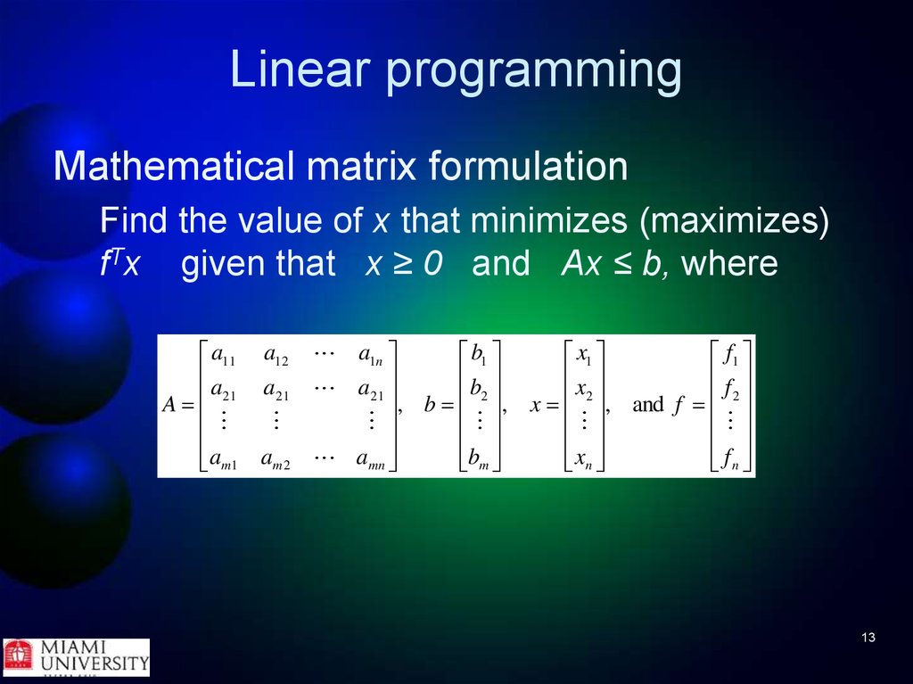
Mathematical matrix formulationFind the value of x that minimizes (maximizes)
fTx given that x ≥ 0 and Ax ≤ b, where
a11
a
A 21
am1
a12
a21
am 2
a1n
b1
x1
f1
b
x
f
a21
2
2
, b , x , and f 2
amn
b
x
m
n
fn
13
14. Linear programming
General procedure1. Restate problem in terms of equations
and inequalities
2. Rewrite in matrix and vector notation
3. Call MATLAB function linprog to solve
14
15. Linear programming
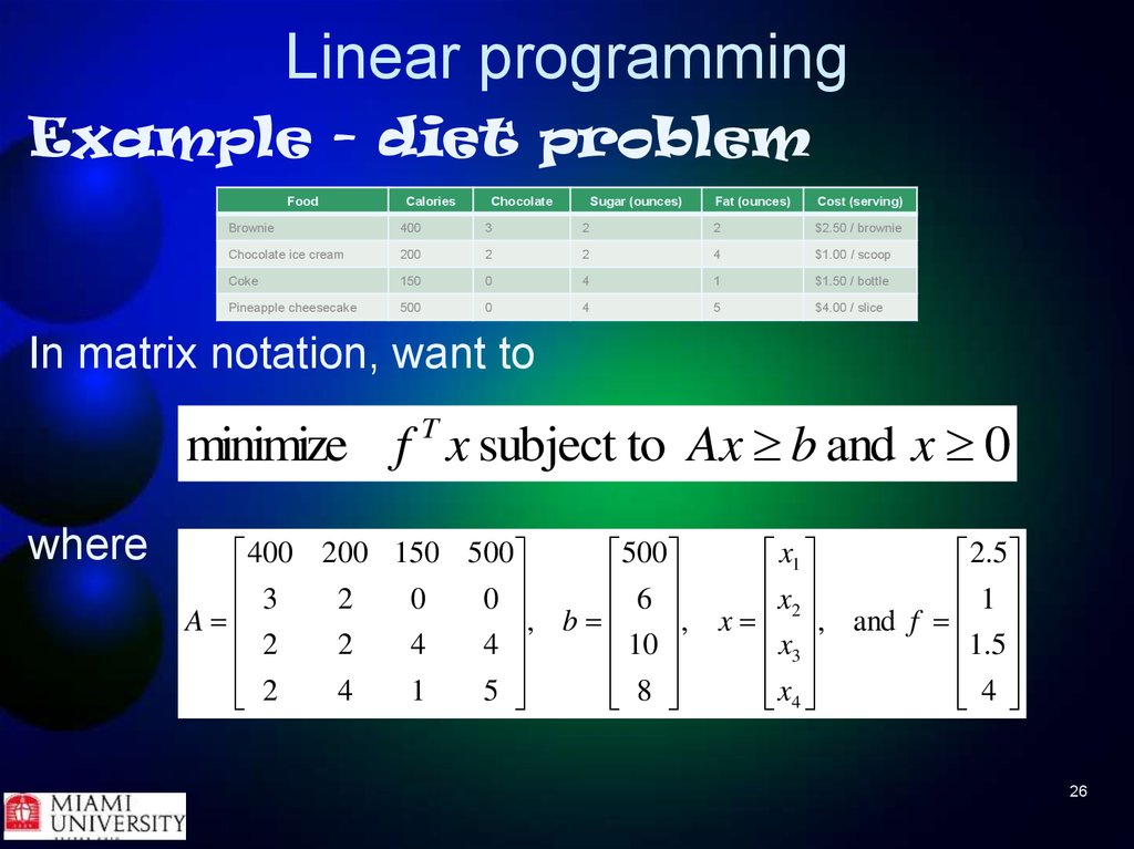
Example - diet problemMy son's diet comes from the four basic food groups chocolate dessert, ice cream, soda, and cheesecake. He
checks in a store and finds one of each kind of food,
namely, a brownie, chocolate ice cream, Pepsi, and one
slice of pineapple cheesecake. Each day he needs at
least 500 calories, 6 oz of chocolate, 10 oz of sugar, and 8
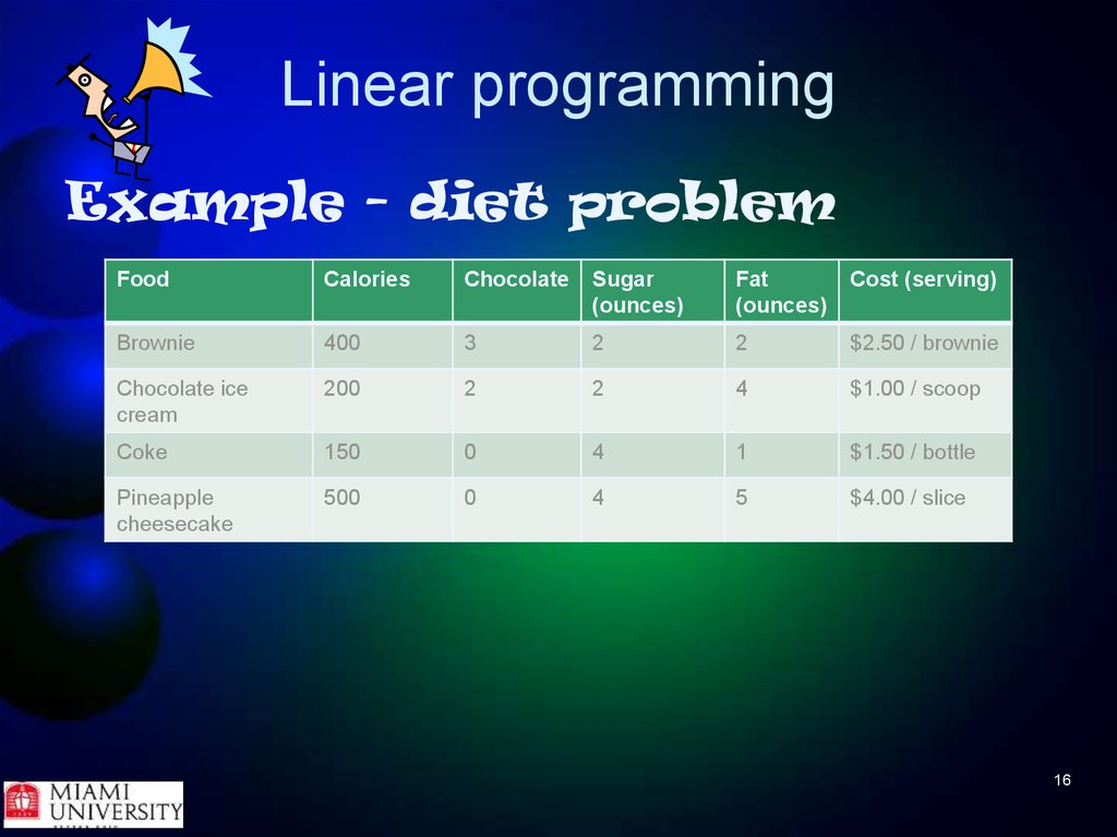
oz of fat. Using the table on the next slide that gives the
cost and nutrition of each item, figure out how much he
should buy and eat of each of the four items he found in
the store so that he gets enough nutrition but spends as
little (of my money...) as possible.
15
16. Linear programming
Example - diet problemFood
Calories
Chocolate
Sugar
(ounces)
Fat
(ounces)
Cost (serving)
Brownie
400
3
2
2
$2.50 / brownie
Chocolate ice
cream
200
2
2
4
$1.00 / scoop
Coke
150
0
4
1
$1.50 / bottle
Pineapple
cheesecake
500
0
4
5
$4.00 / slice
16
17. Linear programming
Example - diet problemFood
Calories
Chocolate
Sugar (ounces)
Fat (ounces)
Cost (serving)
Brownie
400
3
2
2
$2.50 / brownie
Chocolate ice cream
200
2
2
4
$1.00 / scoop
Coke
150
0
4
1
$1.50 / bottle
Pineapple cheesecake
500
0
4
5
$4.00 / slice
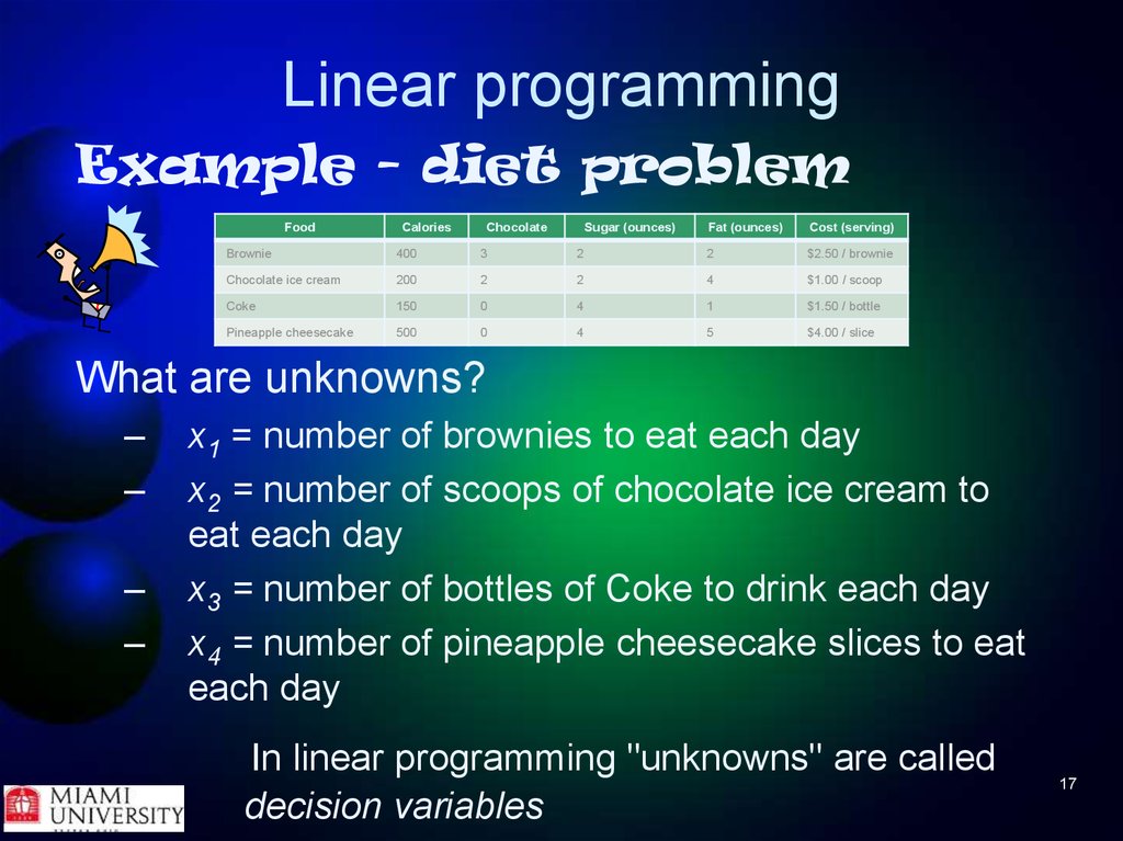
What are unknowns?
–
–
–
–
x1 = number of brownies to eat each day
x2 = number of scoops of chocolate ice cream to
eat each day
x3 = number of bottles of Coke to drink each day
x4 = number of pineapple cheesecake slices to eat
each day
In linear programming "unknowns" are called
decision variables
17
18. Linear programming
Example - diet problemFood
Calories
Chocolate
Sugar (ounces)
Fat (ounces)
Cost (serving)
Brownie
400
3
2
2
$2.50 / brownie
Chocolate ice cream
200
2
2
4
$1.00 / scoop
Coke
150
0
4
1
$1.50 / bottle
Pineapple cheesecake
500
0
4
5
$4.00 / slice
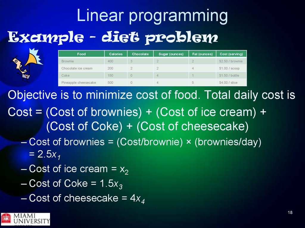
Objective is to minimize cost of food. Total daily cost is
Cost = (Cost of brownies) + (Cost of ice cream) +
(Cost of Coke) + (Cost of cheesecake)
– Cost of brownies = (Cost/brownie) × (brownies/day)
= 2.5x1
– Cost of ice cream = x2
– Cost of Coke = 1.5x3
– Cost of cheesecake = 4x4
18
19. Linear programming
Example - diet problemFood
Calories
Chocolate
Sugar (ounces)
Fat (ounces)
Cost (serving)
Brownie
400
3
2
2
$2.50 / brownie
Chocolate ice cream
200
2
2
4
$1.00 / scoop
Coke
150
0
4
1
$1.50 / bottle
Pineapple cheesecake
500
0
4
5
$4.00 / slice
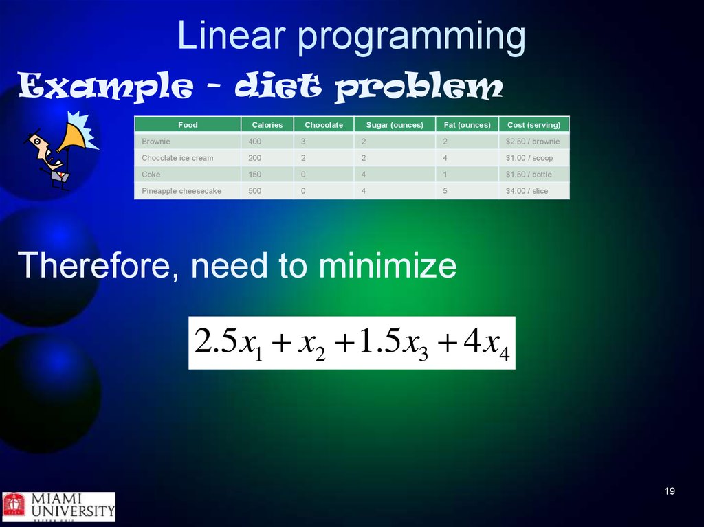
Therefore, need to minimize
2.5x1 x2 1.5 x3 4 x4
19
20. Linear programming
Example - diet problemFood
Calories
Chocolate
Sugar (ounces)
Fat (ounces)
Cost (serving)
Brownie
400
3
2
2
$2.50 / brownie
Chocolate ice cream
200
2
2
4
$1.00 / scoop
Coke
150
0
4
1
$1.50 / bottle
Pineapple cheesecake
500
0
4
5
$4.00 / slice
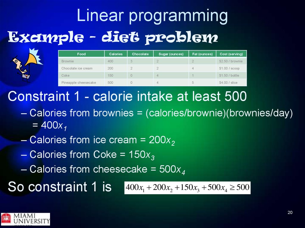
Constraint 1 - calorie intake at least 500
– Calories from brownies = (calories/brownie)(brownies/day)
= 400x1
– Calories from ice cream = 200x2
– Calories from Coke = 150x3
– Calories from cheesecake = 500x4
So constraint 1 is
400 x1 200 x2 150 x3 500 x4 500
20
21. Linear programming
Example - diet problemFood
Calories
Chocolate
Sugar (ounces)
Fat (ounces)
Cost (serving)
Brownie
400
3
2
2
$2.50 / brownie
Chocolate ice cream
200
2
2
4
$1.00 / scoop
Coke
150
0
4
1
$1.50 / bottle
Pineapple cheesecake
500
0
4
5
$4.00 / slice
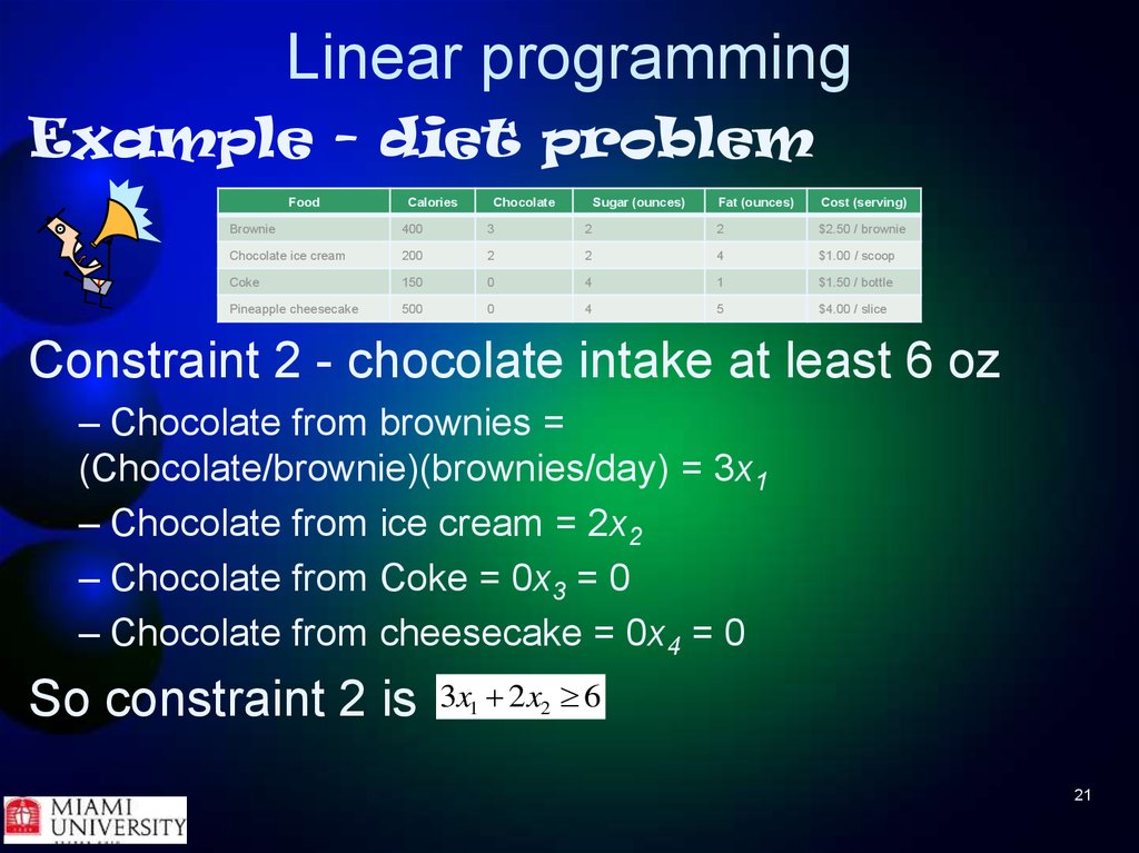
Constraint 2 - chocolate intake at least 6 oz
– Chocolate from brownies =
(Chocolate/brownie)(brownies/day) = 3x1
– Chocolate from ice cream = 2x2
– Chocolate from Coke = 0x3 = 0
– Chocolate from cheesecake = 0x4 = 0
So constraint 2 is
3x1 2x2 6
21
22. Linear programming
Example - diet problemFood
Calories
Chocolate
Sugar (ounces)
Fat (ounces)
Cost (serving)
Brownie
400
3
2
2
$2.50 / brownie
Chocolate ice cream
200
2
2
4
$1.00 / scoop
Coke
150
0
4
1
$1.50 / bottle
Pineapple cheesecake
500
0
4
5
$4.00 / slice
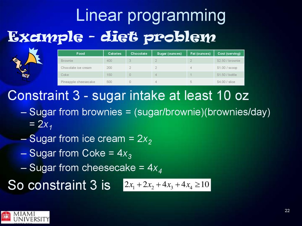
Constraint 3 - sugar intake at least 10 oz
– Sugar from brownies = (sugar/brownie)(brownies/day)
= 2x1
– Sugar from ice cream = 2x2
– Sugar from Coke = 4x3
– Sugar from cheesecake = 4x4
So constraint 3 is
2 x1 2 x2 4 x3 4 x4 10
22
23. Linear programming
Example - diet problemFood
Calories
Chocolate
Sugar (ounces)
Fat (ounces)
Cost (serving)
Brownie
400
3
2
2
$2.50 / brownie
Chocolate ice cream
200
2
2
4
$1.00 / scoop
Coke
150
0
4
1
$1.50 / bottle
Pineapple cheesecake
500
0
4
5
$4.00 / slice
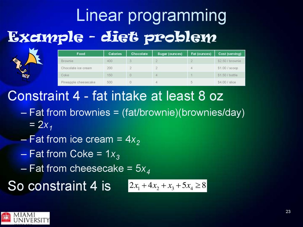
Constraint 4 - fat intake at least 8 oz
– Fat from brownies = (fat/brownie)(brownies/day)
= 2x1
– Fat from ice cream = 4x2
– Fat from Coke = 1x3
– Fat from cheesecake = 5x4
So constraint 4 is
2 x1 4 x2 x3 5x4 8
23
24. Linear programming
Example - diet problemFood
Calories
Chocolate
Sugar (ounces)
Fat (ounces)
Cost (serving)
Brownie
400
3
2
2
$2.50 / brownie
Chocolate ice cream
200
2
2
4
$1.00 / scoop
Coke
150
0
4
1
$1.50 / bottle
Pineapple cheesecake
500
0
4
5
$4.00 / slice
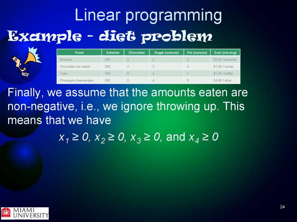
Finally, we assume that the amounts eaten are
non-negative, i.e., we ignore throwing up. This
means that we have
x1 ≥ 0, x2 ≥ 0, x3 ≥ 0, and x4 ≥ 0
24
25. Linear programming
Example - diet problemFood
Calories
Chocolate
Sugar (ounces)
Fat (ounces)
Cost (serving)
Brownie
400
3
2
2
$2.50 / brownie
Chocolate ice cream
200
2
2
4
$1.00 / scoop
Coke
150
0
4
1
$1.50 / bottle
Pineapple cheesecake
500
0
4
5
$4.00 / slice
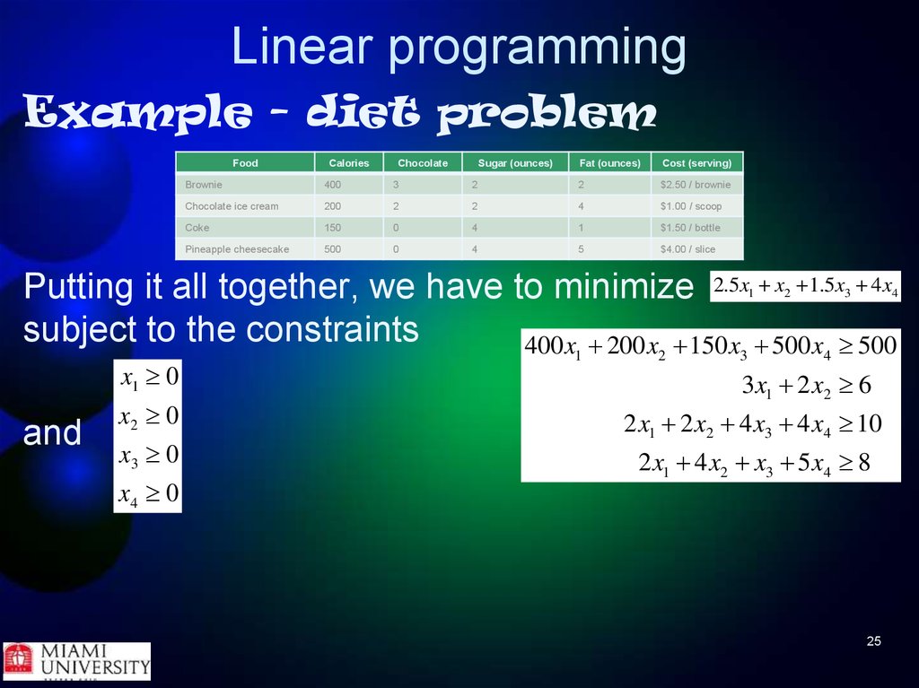
Putting it all together, we have to minimize 2.5x x 1.5x 4x
subject to the constraints
400 x 200 x 150 x 500 x 500
1
x1 0
and
x2 0
x3 0
x4 0
1
2
3
2
3
4
4
3x1 2 x2 6
2 x1 2 x2 4 x3 4 x4 10
2 x1 4 x2 x3 5 x4 8
25
26. Linear programming
Example - diet problemFood
Calories
Chocolate
Sugar (ounces)
Fat (ounces)
Cost (serving)
Brownie
400
3
2
2
$2.50 / brownie
Chocolate ice cream
200
2
2
4
$1.00 / scoop
Coke
150
0
4
1
$1.50 / bottle
Pineapple cheesecake
500
0
4
5
$4.00 / slice
In matrix notation, want to
minimize f x subject to Ax b and x 0
T
where
x1
400 200 150 500
500
2. 5
x
3
6
1
2
0
0
2
, b
, x , and f
A
x3
2
10
1.5
2
4
4
x
2
4
1
5
8
4
4
26
27. Linear programming
MATLAB solves linear programming problemA x b
minimize f T x such that Aeq x beq
lb x ub
where x, b, beq, lb, and ub are vectors and A and Aeq
are matrices.
• Can use one or more of the constraints
• "lb" means "lower bound", "ub" means "upper bound"
– Often have lb = 0 and ub = ∞, i.e., no upper bound
27
28. Linear programming
MATLAB linear programming solver islinprog(), which you can call various ways:
x = linprog(f,A,b)
x = linprog(f,A,b,Aeq,beq)
x = linprog(f,A,b,Aeq,beq,lb,ub)
x = linprog(f,A,b,Aeq,beq,lb,ub,x0)
x = linprog(f,A,b,Aeq,beq,lb,ub,x0,options)
x = linprog(problem)
[x,fval] = linprog(...)
[x,fval,exitflag] = linprog(...)
[x,fval,exitflag,output] = linprog(...)
[x,fval,exitflag,output,lambda] = linprog(...)
28
29. Linear programming
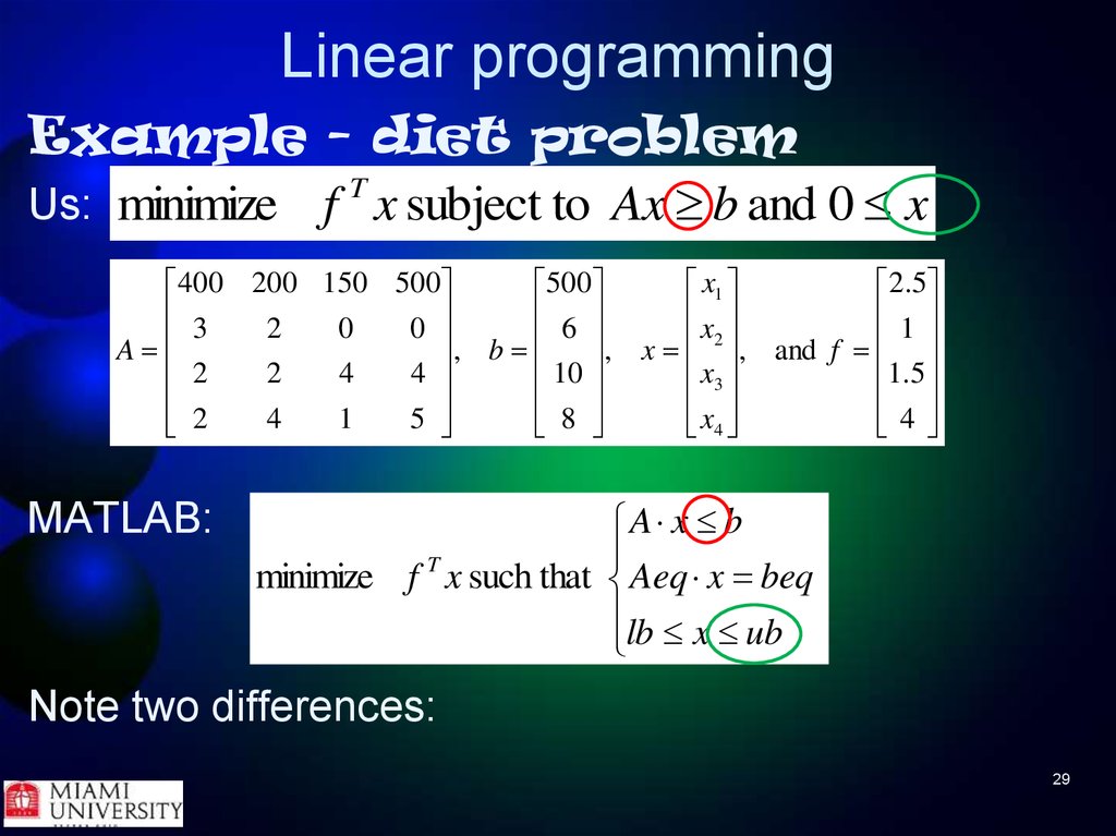
Example - diet problemUs: minimize f T x subject to Ax b and 0 x
x1
400 200 150 500
500
2. 5
x
3
6
1
2
0
0
2
, b
, x , and f
A
x3
2
10
1.5
2
4
4
x
2
4
1
5
8
4
4
MATLAB:
A x b
minimize f T x such that Aeq x beq
lb x ub
Note two differences:
29
30. Linear programming
Example - diet problemISSUE 1 - We have Ax ≥ b but need Ax ≤ b
One way to handle is to note that
if Ax ≥ b then -Ax ≤ -b, so can have MATLAB use
constraint (-A)x ≤ (-b)
ISSUE 2 - We have 0 ≤ x but MATLAB wants
lb ≤ x ≤ ub . Handle by omitting ub in call of
linprog(). If omitted, MATLAB assumes no
upper bound
30
31. Linear programming
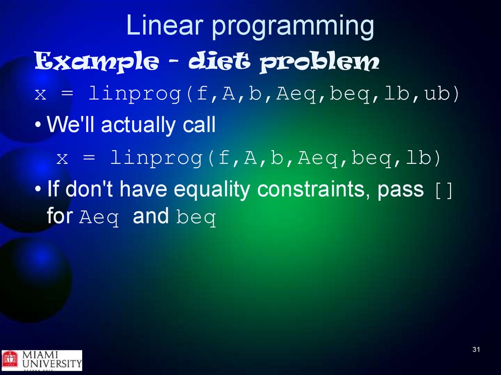
Example - diet problemx = linprog(f,A,b,Aeq,beq,lb,ub)
• We'll actually call
x = linprog(f,A,b,Aeq,beq,lb)
• If don't have equality constraints, pass []
for Aeq and beq
31
32. Linear programming
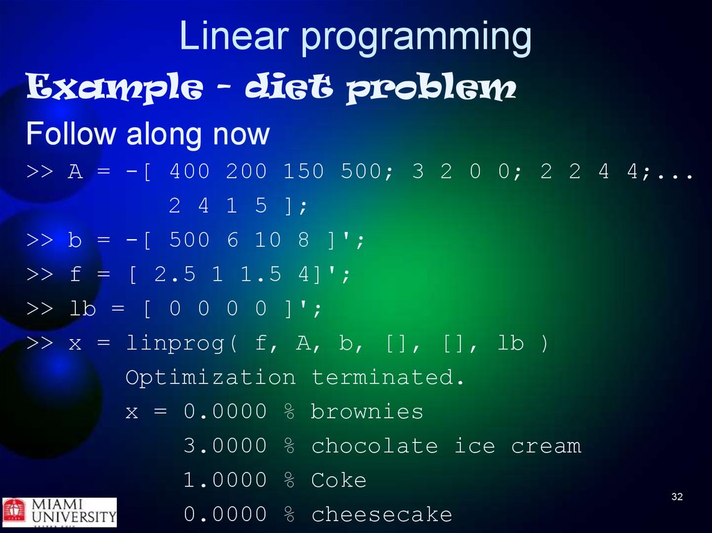
Example - diet problemFollow along now
>> A = -[ 400 200 150 500; 3 2 0 0; 2 2 4 4;...
2 4 1 5 ];
>> b = -[ 500 6 10 8 ]';
>> f = [ 2.5 1 1.5 4]';
>> lb = [ 0 0 0 0 ]';
>> x = linprog( f, A, b, [], [], lb )
Optimization terminated.
x = 0.0000 % brownies
3.0000 % chocolate ice cream
1.0000 % Coke
32
0.0000 % cheesecake
33. Linear programming
Example - diet problemOptimal solution is x = [ 0 3 1 0 ]T . In words,
my son should eat 3 scoops of ice cream and
drink 1 Coke each day.
33
34. Linear programming
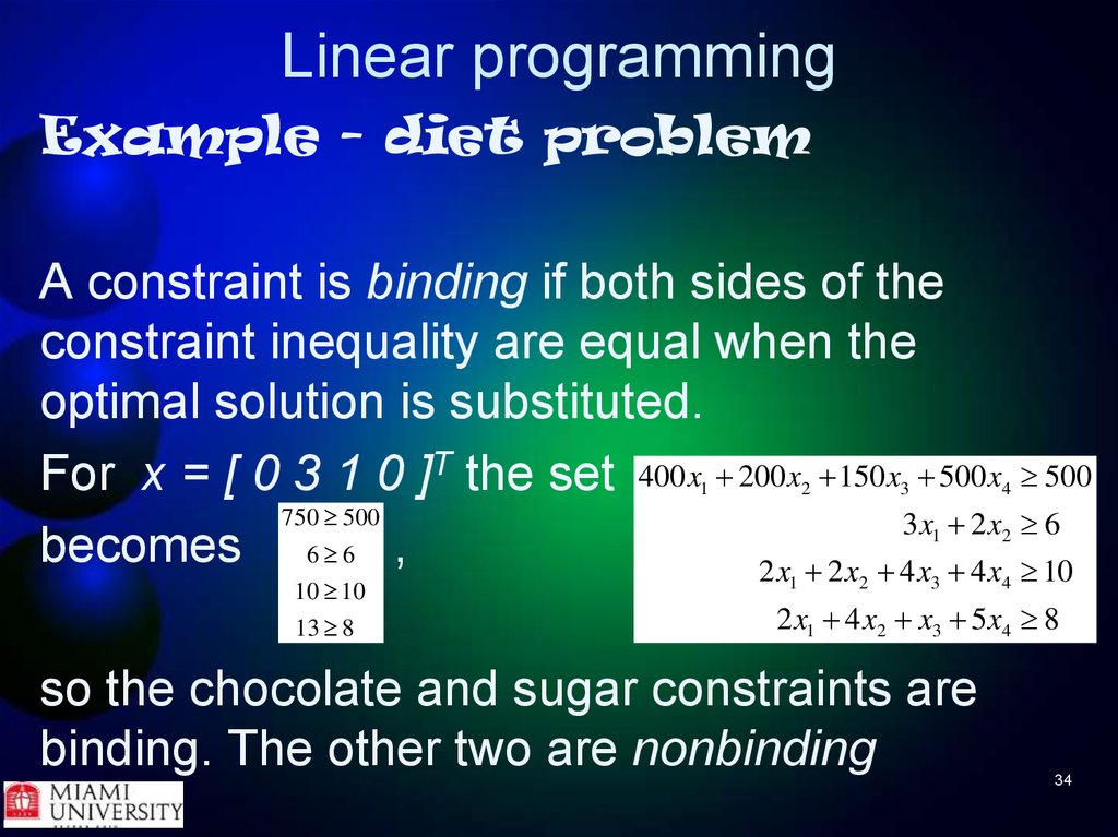
Example - diet problemA constraint is binding if both sides of the
constraint inequality are equal when the
optimal solution is substituted.
For x = [ 0 3 1 0 ]T the set 400 x 200 x 150 x 500 x
750 500
3x 2 x
becomes 6 6 ,
2x 2x 4x 4x
1
10 10
13 8
2
1
4
500
1
2
6
3
4
10
3
2
2 x1 4 x2 x3 5 x4 8
so the chocolate and sugar constraints are
binding. The other two are nonbinding
34
35. Linear programming
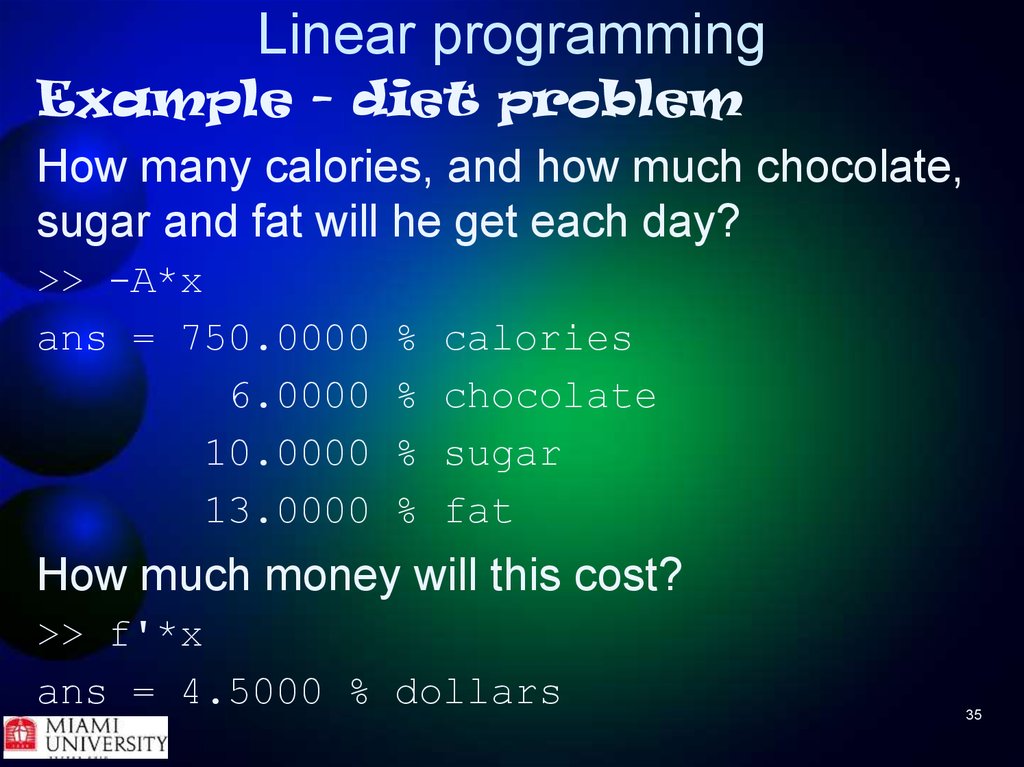
Example - diet problemHow many calories, and how much chocolate,
sugar and fat will he get each day?
>> -A*x
ans = 750.0000
6.0000
10.0000
13.0000
%
%
%
%
calories
chocolate
sugar
fat
How much money will this cost?
>> f'*x
ans = 4.5000 % dollars
35
36. Linear programming
Example - diet problemBecause it's common to want to know the value
of the objective function at the optimum,
linprog() can return that to you
[x fval] = linprog(f,A,b,Aeq,beq,lb,ub)
where fval = fTx
>> [x fval] = linprog( f, A, b, [], [], lb )
x = 0.0000
3.0000
1.0000
0.0000
fval = 4.5000
36
37. Linear programming
Special kinds of solutionsUsually a linear programming problem has a unique
(single) optimal solution. However, there can also be:
1. No feasible solutions
2. An unbounded solution. There are solutions that
make the objective function arbitrarily large (max
problem) or arbitrarily small (min problem)
3. An infinite number of optimal solutions. The
technique of goal programming is often used to
choose among alternative optimal solutions.
(Won't consider this case more)
37
38. Linear programming
Can tell about the solution MATLAB finds byusing third output variable:
[x fval exitflag] =...
linprog(f,A,b,Aeq,beq,lb,ub)
exitflag - integer identifying the reason the algorithm
terminated. Values are
1
0
-2
-3
-4
-5
-7
Function converged to a solution x.
Number of iterations exceeded options.
No feasible point was found.
Problem is unbounded.
NaN value was encountered during execution of the algorithm.
Both primal and dual problems are infeasible.
Search direction became too small. No further progress could be made.
38
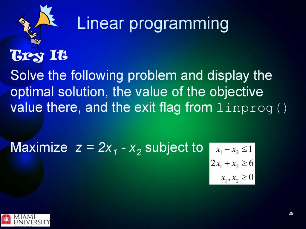
39. Linear programming
Try ItSolve the following problem and display the
optimal solution, the value of the objective
value there, and the exit flag from linprog()
Maximize z = 2x1 - x2 subject to
x1 x2 1
2 x1 x2 6
x1 , x2 0
39
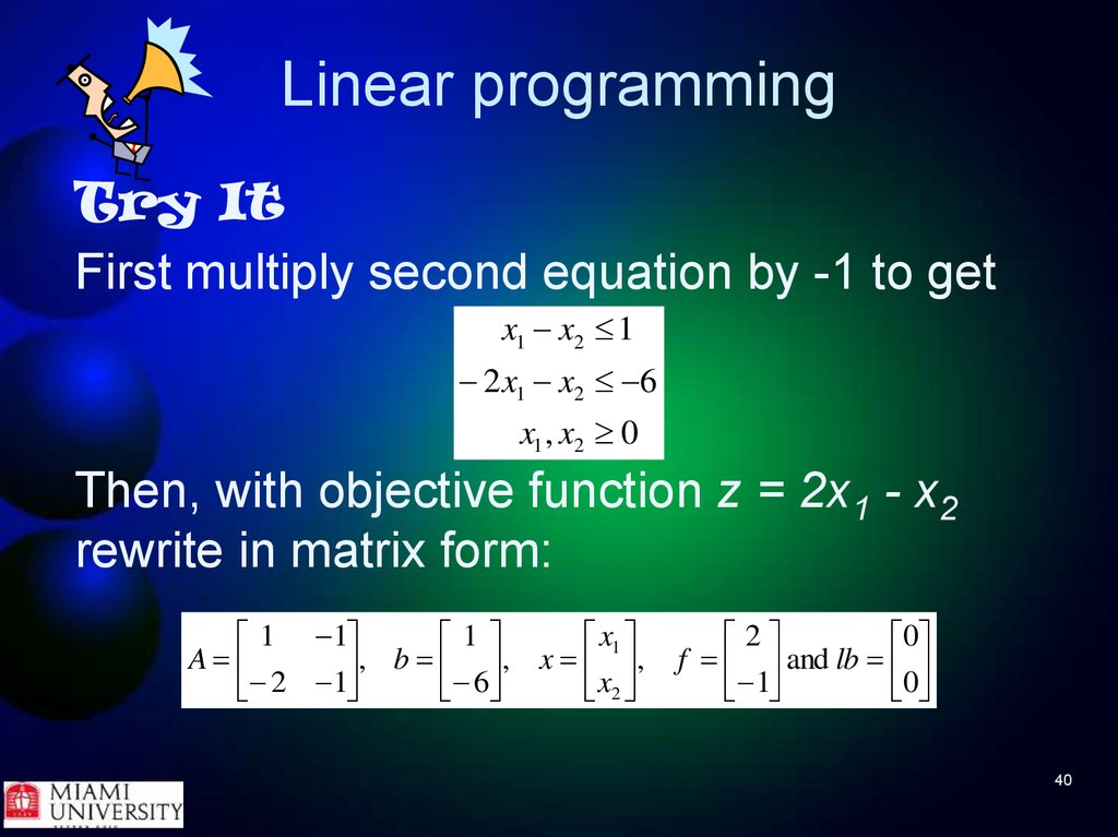
40. Linear programming
Try ItFirst multiply second equation by -1 to get
x1 x2 1
2 x1 x2 6
x1 , x2 0
Then, with objective function z = 2x1 - x2
rewrite in matrix form:
x1
1 1
1
A
, b , x ,
2 1
6
x2
2
0
f and lb
1
0
40
41. Linear programming
Try It>>
>>
>>
>>
x1
1 1
1
2
0
A
, b 6 , x x , f 1 and lb 0
2
1
2
A = [ 1 -1; -2 -1 ];
b = [ 1 -6 ]';
f = [ 2 -1 ]';
lb = [ 0 0 ]';
41
42. Linear programming
Try ItIMPORTANT - linprog() tries to
minimize the objective function. If you
want to maximize the objective function,
pass -f and use -fval as the
maximum value of the objective function
42
43. Linear programming
Try It>> [x fval exitflag] = linprog( -f, A, b, [],[], lb )
Exiting: One or more of the residuals, duality gap,
or total relative error has grown 100000 times
greater than its minimum value so far: the dual
appears to be infeasible (and the primal unbounded).
(The primal residual < TolFun=1.00e-008.)
x = 1.0e+061 *
4.4649
4.4649
fval = -4.4649e+061 (-fval = 4.4649e+061 !!!)
exitflag = -3 (Problem is unbounded)
43
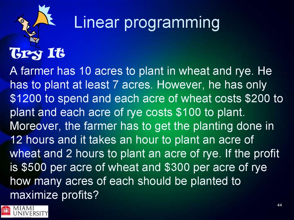
44. Linear programming
Try ItA farmer has 10 acres to plant in wheat and rye. He
has to plant at least 7 acres. However, he has only
$1200 to spend and each acre of wheat costs $200 to
plant and each acre of rye costs $100 to plant.
Moreover, the farmer has to get the planting done in
12 hours and it takes an hour to plant an acre of
wheat and 2 hours to plant an acre of rye. If the profit
is $500 per acre of wheat and $300 per acre of rye
how many acres of each should be planted to
maximize profits?
44
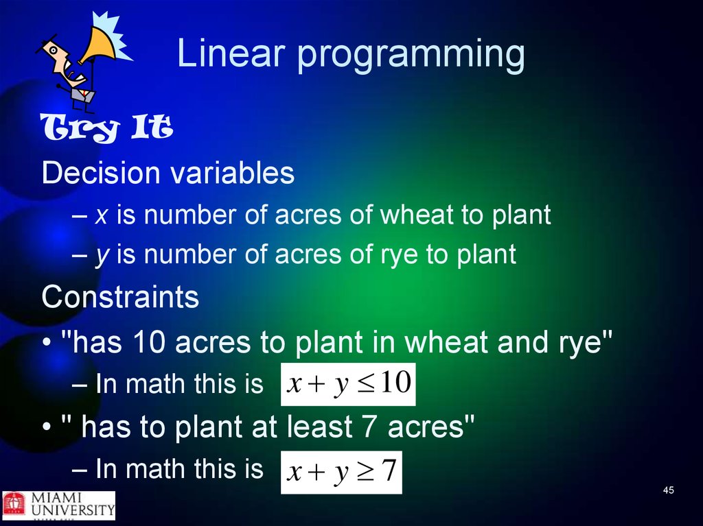
45. Linear programming
Try ItDecision variables
– x is number of acres of wheat to plant
– y is number of acres of rye to plant
Constraints
• "has 10 acres to plant in wheat and rye"
– In math this is x y 10
• " has to plant at least 7 acres"
– In math this is x y 7
45
46. Linear programming
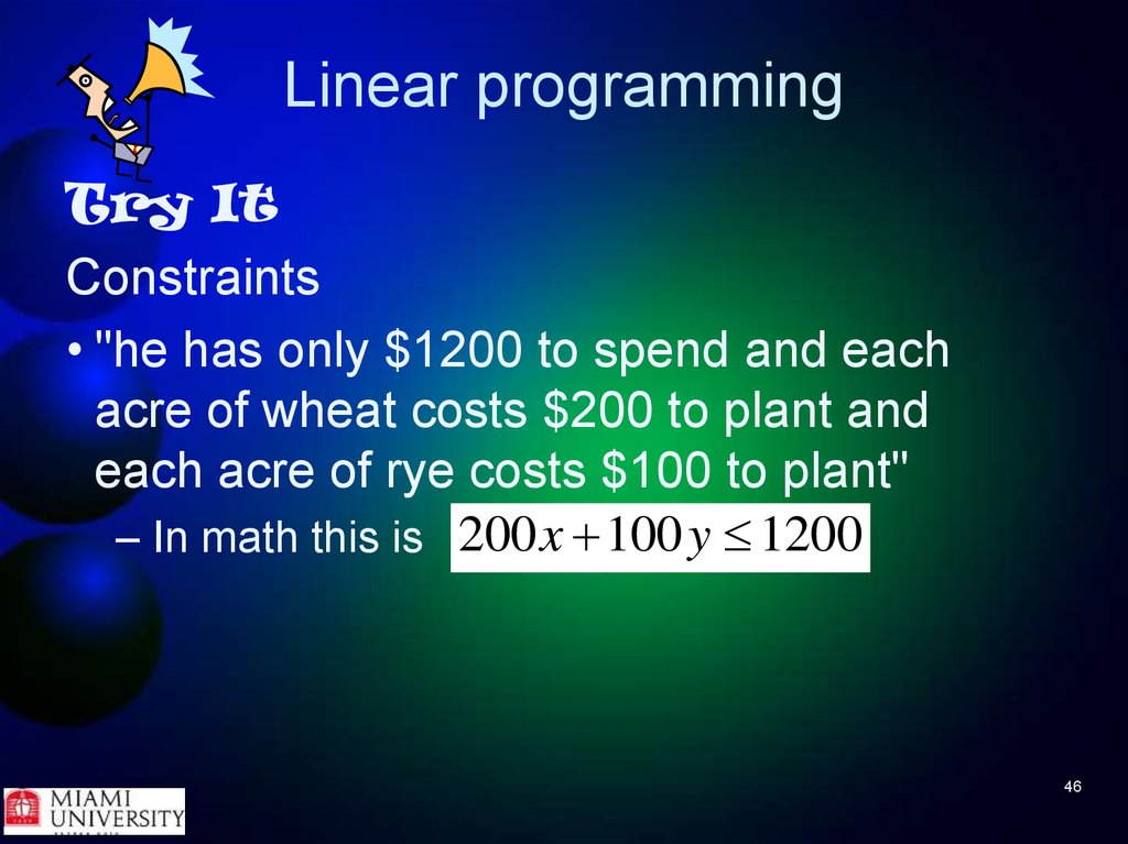
Try ItConstraints
• "he has only $1200 to spend and each
acre of wheat costs $200 to plant and
each acre of rye costs $100 to plant"
– In math this is 200 x 100 y 1200
46
47. Linear programming
Try ItConstraints
• "the farmer has to get the planting done in
12 hours and it takes an hour to plant an
acre of wheat and 2 hours to plant an acre
of rye "
– In math this is 1x 2 y 12
47
48. Linear programming
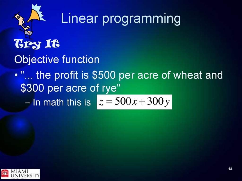
Try ItObjective function
• "... the profit is $500 per acre of wheat and
$300 per acre of rye"
– In math this is z 500 x 300 y
48
49. Linear programming
Try ItPut it together
– Constraints:
x y 10
x y 7
200 x 100 y 1200
x 2 y 12
x 0
y 0
– Objective function:
z 500 x 300 y
49
50. Linear programming
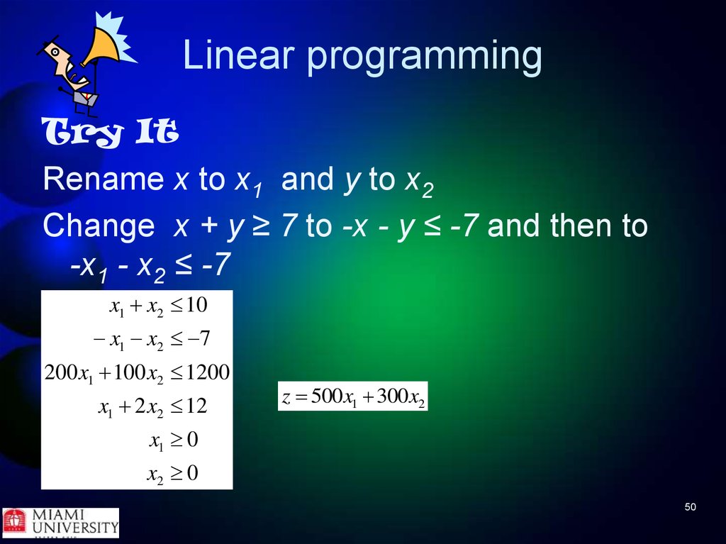
Try ItRename x to x1 and y to x2
Change x + y ≥ 7 to -x - y ≤ -7 and then to
-x1 - x2 ≤ -7
x1 x2 10
x1 x2 7
200 x1 100 x2 1200
x1 2 x2 12
z 500x1 300x2
x1 0
x2 0
50
51. Linear programming
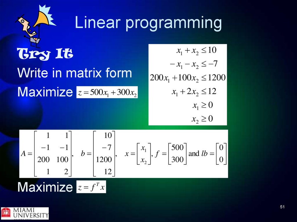
Try ItWrite in matrix form
Maximize z 500x 300x
1
2
x1 x2 10
x1 x2 7
200 x1 100 x2 1200
x1 2 x2 12
x1 0
x2 0
1
1
10
1 1
7
, b
, x x1 , f 500 and lb 0
A
x
300
0
200 100
1200
2
2
1
12
Maximize
z f Tx
51
52. Linear programming
11
10
1 1
, b 7 , x x1 , f 500 and lb 0
A
x
300
0
200 100
1200
2
1
2
12
z f Tx
Try It
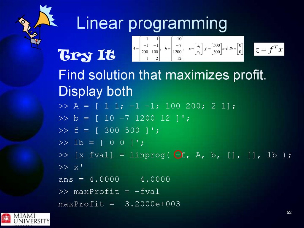
Find solution that maximizes profit.
Display both
>> A = [ 1 1; -1 -1; 100 200; 2 1];
>> b = [ 10 -7 1200 12 ]';
>> f = [ 300 500 ]';
>> lb = [ 0 0 ]';
>> [x fval] = linprog( -f, A, b, [], [], lb );
>> x'
ans = 4.0000
4.0000
>> maxProfit = -fval
maxProfit = 3.2000e+003
52
53. Linear programming
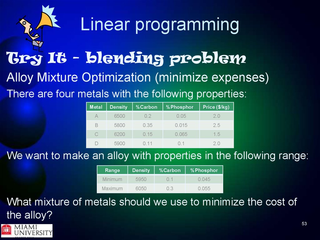
Try It - blending problemAlloy Mixture Optimization (minimize expenses)
There are four metals with the following properties:
Metal
Density
%Carbon
%Phosphor
Price ($/kg)
A
6500
0.2
0.05
2.0
B
5800
0.35
0.015
2.5
C
6200
0.15
0.065
1.5
D
5900
0.11
0.1
2.0
We want to make an alloy with properties in the following range:
Range
Density
%Carbon
%Phosphor
Minimum
5950
0.1
0.045
Maximum
6050
0.3
0.055
What mixture of metals should we use to minimize the cost of
the alloy?
53
54. Linear programming
Try It - blending problemDecision variables
– x1 is fraction of total alloy that is metal A
– x2 is fraction of total alloy that is metal B
– x3 is fraction of total alloy that is metal C
– x4 is fraction of total alloy that is metal D
54
55. Linear programming
MetalDensity
%Carbon
%Phosphor
Price ($/kg)
A
6500
0.2
0.05
2.0
B
5800
0.35
0.015
2.5
C
6200
0.15
0.065
1.5
D
5900
0.11
0.1
2.0
Range
Density
%Carbon
%Phosphor
Minimum
5950
0.1
0.045
Maximum
6050
0.3
0.055
Try It - blending problem
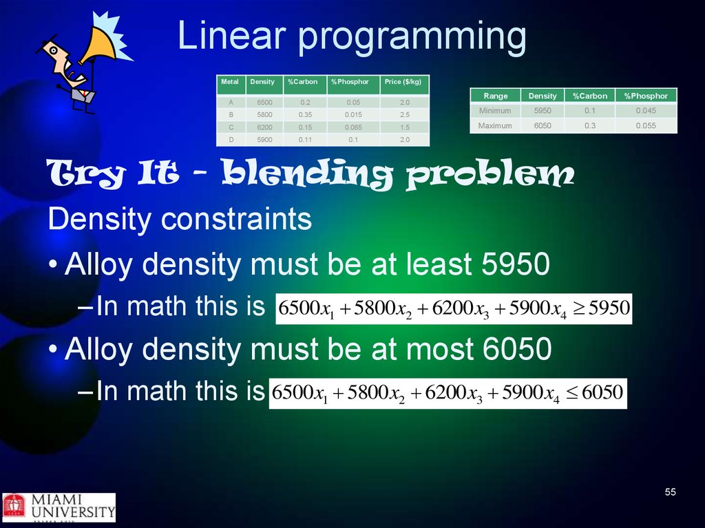
Density constraints
• Alloy density must be at least 5950
–In math this is
6500 x1 5800 x2 6200 x3 5900 x4 5950
• Alloy density must be at most 6050
–In math this is 6500 x1 5800x2 6200x3 5900 x4 6050
55
56. Linear programming
MetalDensity
%Carbon
%Phosphor
Price ($/kg)
A
6500
0.2
0.05
2.0
B
5800
0.35
0.015
2.5
C
6200
0.15
0.065
1.5
D
5900
0.11
0.1
2.0
Range
Density
%Carbon
%Phosphor
Minimum
5950
0.1
0.045
Maximum
6050
0.3
0.055
Try It - blending problem
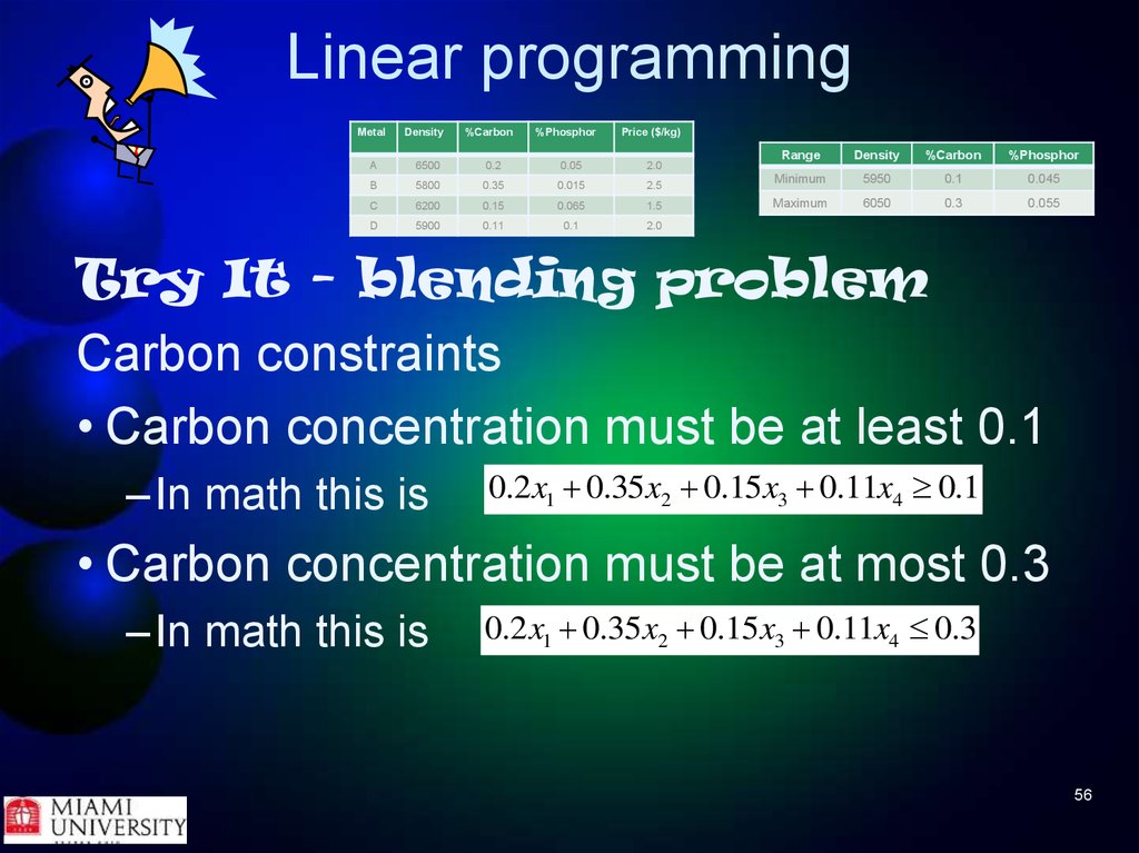
Carbon constraints
• Carbon concentration must be at least 0.1
–In math this is
0.2 x1 0.35 x2 0.15 x3 0.11x4 0.1
• Carbon concentration must be at most 0.3
–In math this is
0.2 x1 0.35 x2 0.15 x3 0.11x4 0.3
56
57. Linear programming
MetalDensity
%Carbon
%Phosphor
Price ($/kg)
A
6500
0.2
0.05
2.0
B
5800
0.35
0.015
2.5
C
6200
0.15
0.065
1.5
D
5900
0.11
0.1
2.0
Range
Density
%Carbon
%Phosphor
Minimum
5950
0.1
0.045
Maximum
6050
0.3
0.055
Try It - blending problem
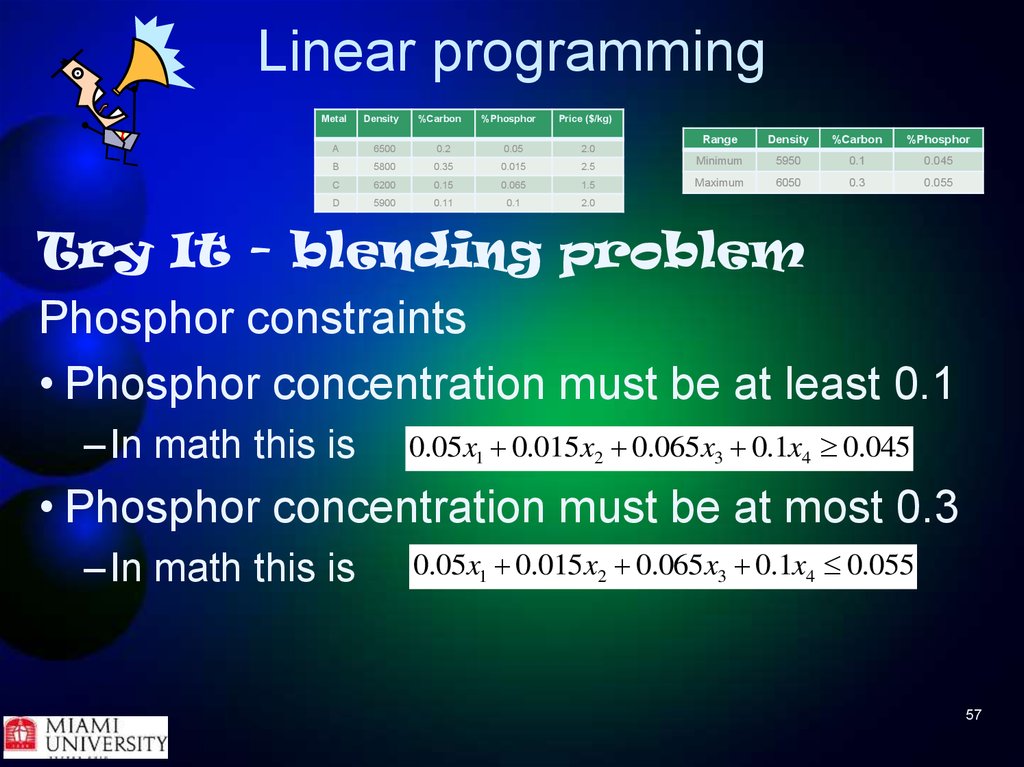
Phosphor constraints
• Phosphor concentration must be at least 0.1
–In math this is
0.05x1 0.015 x2 0.065x3 0.1x4 0.045
• Phosphor concentration must be at most 0.3
–In math this is
0.05x1 0.015 x2 0.065x3 0.1x4 0.055
57
58. Linear programming
Try It - blending problemConstraints
Since only the four metals will make up the
alloy, the sum of the fractional amounts
must be one: x1 x2 x3 x4 1
Fractional parts must be non-negative:
0 xi
for i 1,2,3,4
(Each part must also be ≤ 1, but that's handled by first
equation.)
58
59. Linear programming
MetalDensity
%Carbon
%Phosphor
Price ($/kg)
A
6500
0.2
0.05
2.0
B
5800
0.35
0.015
2.5
C
6200
0.15
0.065
1.5
D
5900
0.11
0.1
2.0
Try It - blending problem
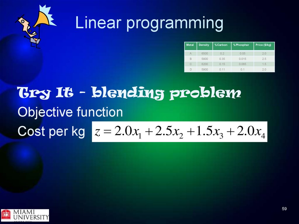
Objective function
Cost per kg z 2.0 x1 2.5x2 1.5 x3 2.0 x4
59
60. Linear programming
Try It - blending problemPut it together 6500 x 5800 x 6200 x 5900 x 5950
1
– Constraints:
(Convert ≥ to ≤)
2
3
4
6500 x1 5800 x2 6200 x3 5900 x4 6050
0.2 x1 0.35 x2 0.15 x3 0.11x4 0.1
0.2 x1 0.35 x2 0.15 x3 0.11x4 0.3
0.05 x1 0.015 x2 0.065 x3 0.1x4 0.045
0.05 x1 0.015 x2 0.065 x3 0.1x4 0.055
x1 x2 x3 x4 1
xi 0, i 1,2,3,4
–Objective function:
z 2.0 x1 2.5x2 1.5x3 2.0 x4
60
61. Linear programming
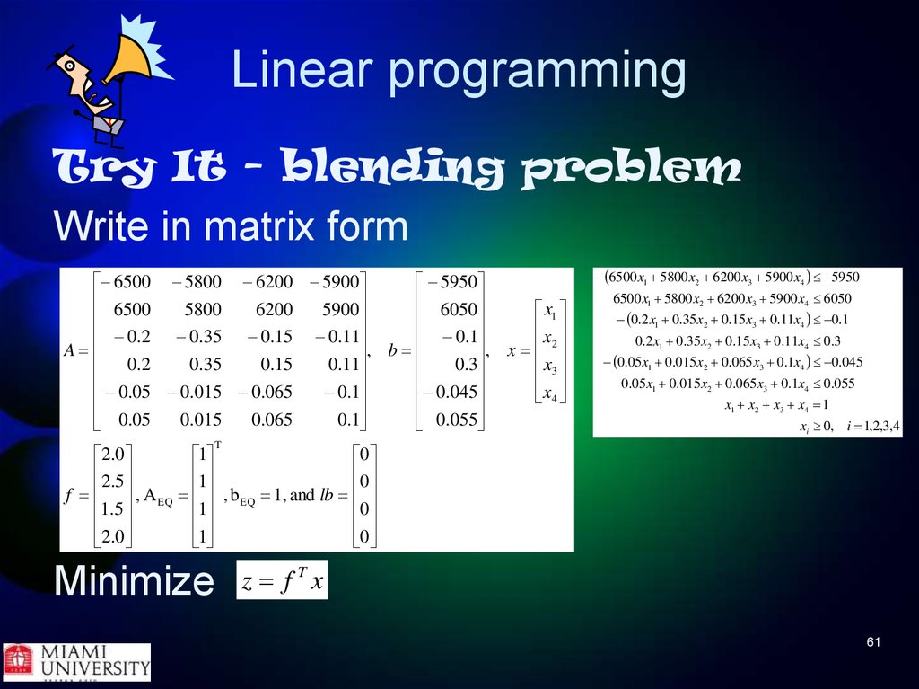
Try It - blending problemWrite in matrix form
6500 5800 6200 5900
5950
6500
6050
5800
6200
5900
x1
x
0.2 0.35 0.15 0.11
0.1
2
A
, b
, x
x3
0.35
0.15
0.11
0.3
0.2
0.05 0.015 0.065
0.045
0.1
x4
0.015
0.065
0.1
0.05
0.055
6500 x1 5800 x2 6200 x3 5900 x4 5950
6500 x1 5800 x2 6200 x3 5900 x4 6050
0.2 x1 0.35 x2 0.15 x3 0.11x4 0.1
0.2 x1 0.35 x2 0.15 x3 0.11x4 0.3
0.05 x1 0.015 x2 0.065 x3 0.1x4 0.045
0.05 x1 0.015 x2 0.065 x3 0.1x4 0.055
x1 x2 x3 x4 1
xi 0, i 1,2,3,4
T
2.0
1
0
2.5
1
0
f , A EQ , b EQ 1, and lb
1.5
1
0
2.0
1
0
Minimize
z f Tx
61
62. Linear programming
6500 5800 6200 59005950
6500
6050
5800
6200
5900
x1
x
0.2 0.35 0.15 0.11
0.1
2
A
,
b
,
x
x3
0
.
2
0
.
35
0
.
15
0
.
11
0
.
3
0.05 0.015 0.065
0.045
0.1
x4
0.015
0.065
0.1
0.05
0.055
T
2.0
1
0
2.5
1
0
f , A EQ , b EQ 1, and lb
1.5
1
0
2.0
1
0
Try It - blending problem
>> A = [-6500 -5800 -6200 -5900; 6500 5800 6200 5900;...
-0.2 -0.35 -0.15 -0.11; 0.2 0.35 0.15 0.11;...
-0.05 -0.015 -0.065 -0.1; 0.05 0.015 0.065 0.1 ];
>> b = [ -5950 6050 -0.1 0.3 -0.045 0.055 ]';
>> f = [ 2 2.5 1.5 2 ]';
>> Aeq = [ 1 1 1 1 ];
>> beq = 1;
>> lb = [ 0 0 0 0 ]';
62
63. Linear programming
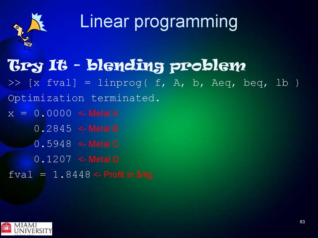
Try It - blending problem>> [x fval] = linprog( f, A, b, Aeq, beq, lb )
Optimization terminated.
x = 0.0000 <- Metal A
0.2845 <- Metal B
0.5948 <- Metal C
0.1207 <- Metal D
fval = 1.8448 <- Profit in $/kg
63
64. MATLAB Linear Programming
Questions?64

























 mathematics
 programming


