Linear Algebra. Chapter 3. Determinants

1. Chapter 3 Determinants

Linear Algebra
Chapter 3
Determinants

2. 3.1 Introduction to Determinants

Definition
The determinant of a 2 2 matrix A is denoted |A| and is given
by
a11
a12
a21
a22
a11a22 a12 a21
Observe that the determinant of a 2 2 matrix is given by the
different of the products of the two diagonals of the matrix.
The notation det(A) is also used for the determinant of A.
Example 1
A 2 4
3 1
det( A) 2 4 (2 1) (4 ( 3)) 2 12 14
3 1
Ch03_2

3.

Definition
Let A be a square matrix.
The minor of the element aij is denoted Mij and is the determinant
of the matrix that remains after deleting row i and column j of A.
The cofactor of aij is denoted Cij and is given by
Cij = (–1)i+j Mij
Note that Cij = Mij or Mij .
Ch03_3

4. Example 2

Determine the minors and cofactors of the elements a11 and a32
of the following matrix A.
0 3
1
A 4 1 2
0 2 1
Solution
1
0 3
Minor of a11 : M 11 4 1 2 1 2 ( 1 1) (2 ( 2)) 3
0 2 1 2 1
Cofactor of a11 : C11 ( 1)1 1 M 11 ( 1) 2 (3) 3
1
0 3
Minor of a32 : M 32 4 1 2 1 3 (1 2) (3 4) 10
0 2 1 4 2
Cofactor of a32 : C32 ( 1)3 2 M 32 ( 1)5 ( 10) 10
Ch03_4

5.

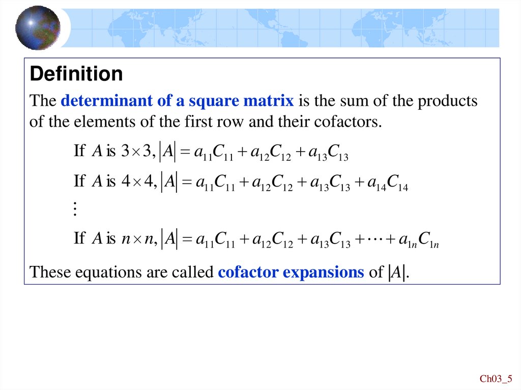
Definition
The determinant of a square matrix is the sum of the products
of the elements of the first row and their cofactors.
If A is 3 3, A a11C11 a12C12 a13C13
If A is 4 4, A a11C11 a12C12 a13C13 a14C14
If A is n n, A a11C11 a12C12 a13C13 a1nC1n
These equations are called cofactor expansions of |A|.
Ch03_5

6. Example 3

Evaluate the determinant of the following matrix A.
1 2 1
A 3 0
1
1
4 2
Solution
A a11C11 a12C12 a13C13
1( 1) 2 0 1 2( 1)3 3 1 ( 1)( 1) 4 3 0
2 1
4 1
4 2
[(0 1) (1 2)] 2[(3 1) (1 4)] [(3 2) (0 4)]
2 2 6
6
Ch03_6

7. Theorem 3.1

The determinant of a square matrix is the sum of the products of
the elements of any row or column and their cofactors.
A ai1Ci1 ai 2Ci 2 ain Cin
ith row expansion:
jth column expansion: A a1 j C1 j a2 j C2 j anjCnj
Example 4
Find the determinant of the following matrix using the second row.
1 2 1
A 3 0
1
1
4 2
Solution
A a21C21 a22C22 a23C23
3 2 1 0 1 1 1 1 2
2
1
4
1 4 2
3[(2 1) ( 1 2)] 0[(1 1) ( 1 4)] 1[(1 2) (2 4)]
12 0 6 6
Ch03_7

8. Example 5

Evaluate the determinant of the following 4 4 matrix.
1
2
0 1
7 2
1
0
0
4
0
2
3
5
0 3
Solution
A a13C13 a23C23 a33C33 a43C43
0(C13 ) 0(C23 ) 3(C33 ) 0(C43 )
2
1
4
3 0 1
2
0
1 3
2 6(3 2) 6
3(2) 1
1 3
Ch03_8

9. Example 6

Solve the following equation for the variable x.
x x 1 7
1 x 2
Solution
Expand the determinant to get the equation
x( x 2) ( x 1)( 1) 7
Proceed to simplify this equation and solve for x.
x2 2x x 1 7
x2 x 6 0
( x 2)( x 3) 0
x 2 or 3
There are two solutions to this equation, x = – 2 or 3.
Ch03_9

10. Computing Determinants of 2  2 and 3  3 Matrices

Computing Determinants of 2 2
and 3 3 Matrices
a11
A
a21
a12
a22 A a11a22 a12 a21
a11
A a21
a
31
a12
a22
a32
a13
a11
a23 a21
a
a33
31
a12
a22
a32
a13 a11
a23 a21
a33 a31
a12
a22
a32
A a11a22 a33 a12 a23a31 a13a21a32
(diagonal products from left to right)
a13a22 a31 a11a23a32 a12 a21a33
(diagonal products from right to left)
Ch03_10

11. Homework

Exercises will be given by the teachers of
the practical classes.
Ch03_11

12. 3.2 Properties of Determinants

Theorem 3.2
Let A be an n n matrix and c be a nonzero scalar.
(a) If A B then |B| = c|A|.
cRk
(b) If A B then |B| = –|A|.
Ri Rj
(c) If A B then |B| = |A|.
Ri cRj
Proof (a)
|A| = ak1Ck1 + ak2Ck2 + … + aknCkn
|B| = cak1Ck1 + cak2Ck2 + … + caknCkn
|B| = c|A|.
Ch03_12

13. Example 1

4 2
3
Evaluate the determinant 1 6
3.
9 3
2
Solution
3
4 2
1 6
2
3
9 3
3 0 2
C2 2 C3
1 0
3 ( 3)
2 3 3
3
2
1
3
21
Ch03_13

14. Example 2

4 3
1
2 5 , |A| = 12 is known.
If A 0
2 4 10
Evaluate the determinants of the following matrices.
4 3
1 12 3
1
1 4 3
(a ) B1 0
6 5 (b) B2 2 4 10 (c) B3 0 2 5
2 12 10
0
0 4 16
2 5
Solution
(a) A B1 Thus |B1| = 3|A| = 36.
3C 2
(b) A
(c)
B2 Thus |B2| = – |A| = –12.
R 2 R 3
A B3 Thus |B3| = |A| = 12.
R 3 2 R1
Ch03_14

15. Theorem 3.3

Definition
A square matrix A is said to be singular if |A|=0.
A is nonsingular if |A| 0.
Theorem 3.3
Let A be a square matrix. A is singular if
(a) all the elements of a row (column) are zero.
(b) two rows (columns) are equal.
(c) two rows (columns) are proportional. (i.e., Ri=cRj)
Proof
(a) Let all elements of the kth row of A be zero.
A ak 1Ck 1 ak 2Ck 2 akn Ckn 0Ck 1 0Ck 2 0Ckn 0
(c) If Ri=cRj, then
|A|=|B|=0
A B , row i of B is [0 0 … 0].
Ri cRj
Ch03_15

16. Example 3

Show that the following matrices are singular.
2 0 7
2 1 3
(a ) A 3 0
1 (b) B 1 2 4
4 0
2 4 8
9
Solution
(a) All the elements in column 2 of A are zero. Thus |A| = 0.
(b) Row 2 and row 3 are proportional. Thus |B| = 0.
Ch03_16

17. Theorem 3.4

Let A and B be n n matrices and c be a nonzero scalar.
(a) |cA| = cn|A|.
(b) |AB| = |A||B|.
(c) |At| = |A|.
1
1
(d) A A (assuming A–1 exists)
Proof
(a)
(d)
A
cR1, cR 2, ..., cRn
A A
1
cA cA c n A
A A
1
I 1
A
1
1
A
Ch03_17

18. Example 4

If A is a 2 2 matrix with |A| = 4, use Theorem 3.4 to compute
the following determinants.
(a) |3A|
(b) |A2|
(c) |5AtA–1|, assuming A–1 exists
Solution
(a) |3A| = (32)|A| = 9 4 = 36.
(b) |A2| = |AA| =|A| |A|= 4 4 = 16.
1
(c) |5AtA–1| = (52)|AtA–1| = 25|At||A–1| 25 A 25.
A
Example 5
Prove that |A–1AtA| = |A|
Solution
1
1
1
A A A (A A )A A A A A
t
t
t
1
1
A A
AA A
A
t
Ch03_18

19. Example 6

Prove that if A and B are square matrices of the same size, with A
being singular, then AB is also singular. Is the converse true?
Solution
( )
( )
|A| = 0 |AB| = |A||B| = 0
Thus the matrix AB is singular.
|AB| = 0 |A||B| = 0 |A| = 0 or |B| = 0
Thus AB being singular implies that either A or B is singular.
The inverse is not true.
Ch03_19

20. Homework

Exercises will be given by the teachers of
the practical classes.
Exercise 11
Prove the following identity without evaluating the determinants.
a b c d e f
a b c d
a c e
q
r
u
v
w
( a b)
q
r
v
w
p
q
r
u
v
w
f
p q r p q r
p
e f
b d
u v w
(c d )
u v w
p
r
u
w
(e f )
p q
u
v
Ch03_20

21. 3.3 Numerical Evaluation of a Determinant

Definition
A square matrix is called an upper triangular matrix if all the
elements below the main diagonal are zero.
It is called a lower triangular matrix if all the elements above the
main diagonal are zero.
1 4 0
3 8 2
0 1 5 , 0 2 3
0 0 0
0 0 9
0 0 0
upper triangular
7
5
9
1
8 0 0
7 0 0
2 1 0 , 1 4 0
7 0 2
3 9 8
4 5 8
lower triangular
0
0
0
1
Ch03_21

22.

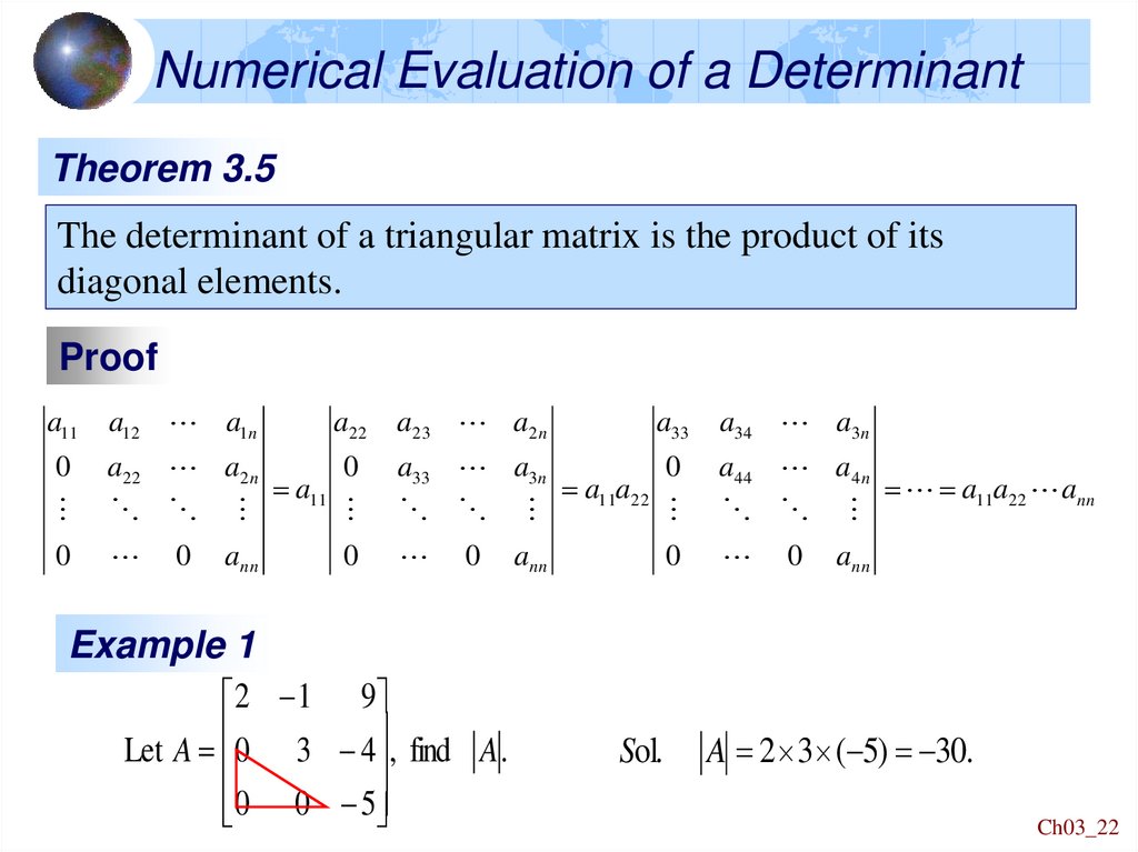
Numerical Evaluation of a Determinant
Theorem 3.5
The determinant of a triangular matrix is the product of its
diagonal elements.
Proof
a11
a12 a1n
0
a22 a2 n
0
ann
0
a11
a22
a23 a2 n
0
a33 a3n
0
ann
0
a33
a34 a3n
0
a44 a4 n
0
ann
a11a22
0
a11a22 ann
Example 1
2 1 9
Let A 0 3 4 , find A .
0 0 5
Sol.
A 2 3 ( 5) 30.
Ch03_22

23. Numerical Evaluation of a Determinant

Example 2
4 1
2
Evaluation the determinant. 2 5 4
9 10
4
Solution (elementary row operations
2
4
1
2
4
2
5
4
R2 R1
0
1 5
9 10 R 3 ( 2) R1 0
1 8
4
2
4
R3 R 2 0 1
0
1
1 2 ( 1) 13 26
5
0 13
Ch03_23

24. Example 3

1 0
2 1
Evaluation the determinant.
1 0
1 0
2
1
0
2
1
0
3
1
2
1
Solution
1
0 2 1
1
0
2 1 1 0 R2 ( 2)R1 0 1 3 2
1
0 0 3 R3 ( 1)R1 0
1
0 2 1
R4 R1
0
1
0
0 2
2
0
2
4
2
1
0 1 3 2
R4 2R3 0
0
0 2
2
0
6
0
1 ( 1) ( 2) 6 12
Ch03_24

25. Example 4

1 2
4
2 5
Evaluation the determinant. 1
2 2 11
Solution
1 2
4
1 2 4
1
2 5 R2 R1 0
0 1
2 2 11 R 3 ( 2)R1 0
2 3
R2 R3
1 2
( 1) 0
0
2
4
3
0 1
( 1) 1 2 ( 1) 2
Ch03_25

26. Example 5

1 1
1
1
Evaluation the determinant.
2 2
6 6
0
2
3
5
2
3
4
1
Solution
1
1 0 2
1 1 0
2
1
1 2 3
R2 R1
0
0 2
2 2 3 4 R3 ( 2)R1 0
0 3
5 0
0
6 6 5 1 R4 ( 6)R1 0
0 5 11
diagonal element is zero and
all elements below this
diagonal element are zero.
Ch03_26

27. 3.4 Determinants, Matrix Inverse, and Systems of Linear Equations

Definition
Let A be an n n matrix and Cij be the cofactor of aij.
The matrix whose (i, j)th element is Cij is called the matrix of
cofactors of A.
The transpose of this matrix is called the adjoint of A and is
denoted adj(A).
C11 C12 C1n
C
C
C
22
2n
21
C
C
C
n2
nn
n1
matrix of cofactors
C11 C12 C1n
C
C
C
22
2n
21
C
C
C
n2
nn
n1
adjoint matrix
t
Ch03_27

28. Example 1

Give the matrix of cofactors and the adjoint matrix of the
following matrix A.
0
3
2
A 1
4 2
5
1 3
Solution The cofactors of A are as follows.
4 1
C11 4 2 14 C12 1 2 3 C13 1
3
5
1
5
1 3
0 6
C21 0 3 9 C22 2 3 7
C23 2
3 5
1 5
1 3
2
3
0
3
2 0 8
C31
12 C32
C
1
33
4 2
1 4
1 2
The matrix of cofactors
The adjoint of A is
of A is 14 3 1
14 9 12
9 7
adj( A) 3
7
1
6
6
8
1
12 1 8
Ch03_28

29. Theorem 3.6

Let A be a square matrix with |A| 0. A is invertible with
1
1
A adj( A)
A
Proof
Consider the matrix product A adj(A). The (i, j)th element of this
product is
(i, j ) th element (row i of A) (column j of adj( A))
C j1
C j 2
ai1 ai 2 ain
C jn
ai1C j1 ai 2C j 2 ain C jn
Ch03_29

30.

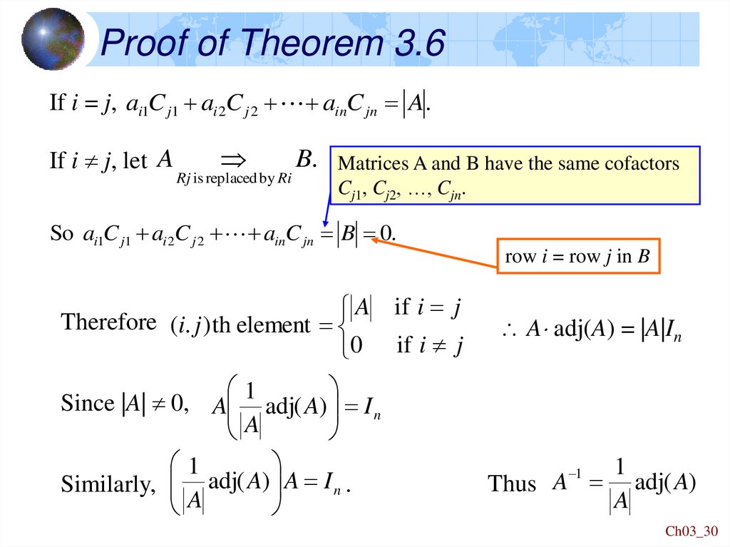
Proof of Theorem 3.6
If i = j, ai1C j1 ai 2C j 2 ainC jn A .
If i j, let A
Rj is replaced by Ri
B.
Matrices A and B have the same cofactors
Cj1, Cj2, …, Cjn.
So ai1C j1 ai 2C j 2 ainC jn B 0.
row i = row j in B
A
Therefore (i. j ) th element
0
1
Since |A| 0, A adj( A) I n
A
1
Similarly, adj( A) A I n .
A
if i j
if i j
A adj(A) = |A|In
1
Thus A adj( A)
A
1
Ch03_30

31. Theorem 3.7

A square matrix A is invertible if and only if |A| 0.
Proof
( ) Assume that A is invertible.
AA–1 = In.
|AA–1| = |In|.
|A||A–1| = 1
|A| 0.
( ) Theorem 3.6 tells us that if |A| 0, then A is invertible.
A–1 exists if and only if |A| 0.
Ch03_31

32. Example 2

Use a determinant to find out which of the following matrices are
invertible.
2 4 3
1 2 1
1
1
4
2
A
B
C 4 12 7 D 1 1 2
3 2
2 1
1
1 0
2 8 0
Solution
|A| = 5 0. A is invertible.
|B| = 0.
B is singular. The inverse does not exist.
|C| = 0.
C is singular. The inverse does not exist.
|D| = 2 0. D is invertible.
Ch03_32

33. Example 3

Use the formula for the inverse of a matrix to compute the inverse
0
3
2
of the matrix
A 1
4 2
5
1 3
Solution
|A| = 25, so the inverse of A exists.We found adj(A) in Example 1
14 9 12
adj( A) 3
7
1
6
8
1
14
1
1
A 1 adj( A) 3
A
25
1
9
7
6
14
12 25
3
1
25
8 1
25
9
25
7
25
6
25
12
25
1
25
8
25
Ch03_33

34. Homework

Exercises will be given by the teachers of
the practical classes.
Exercise
Show that if A = A-1, then |A| = 1.
Show that if At = A-1, then |A| = 1.
Ch03_34

35. Theorem 3.8

Let AX = B be a system of n linear equations in n variables.
(1) If |A| 0, there is a unique solution.
(2) If |A| = 0, there may be many or no solutions.
Proof
(1) If |A| 0
A–1 exists (Thm 3.7)
there is then a unique solution given by X = A–1B (Thm 2.9).
(2) If |A| = 0
since A C implies that if |A| 0 then |C| 0 (Thm 3.2).
the reduced echelon form of A is not In.
The solution to the system AX = B is not unique.
many or no solutions.
Ch03_35

36. Example 4

Determine whether or not the following system of equations has
an unique solution.
3 x1 3 x2 2 x3 2
4 x1 x2 3 x3 5
7 x1 4 x2 x3 9
Solution
Since
3 3 2
4 1
3 0
7 4
1
Thus the system does not have an unique solution.
Ch03_36

37. Theorem 3.9 Cramer’s Rule

Let AX = B be a system of n linear equations in n variables such
that |A| 0. The system has a unique solution given by
A1
A2
An
x1
, x2
, ... , xn
A
A
A
Where Ai is the matrix obtained by replacing column i of A with B.
Proof
|A| 0 the solution to AX = B is unique and is given by
X A 1 B
1
adj( A) B
A
Ch03_37

38.

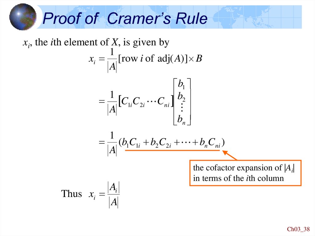
Proof of Cramer’s Rule
xi, the ith element of X, is given by
1
xi [row i of adj( A)] B
A
b1
1
C1i C2i Cni b2
A
b
n
1
(b1C1i b2C2i bnCni )
A
Ai
Thus xi
A
the cofactor expansion of |Ai|
in terms of the ith column
Ch03_38

39. Example 5

Solving the following system of equations using Cramer’s rule.
x1 3 x2 x3 2
2 x1 5 x2 x3 5
x1 2 x2 3 x3 6
Solution
The matrix of coefficients A and column matrix of constants B are
1 3 1
2
A 2 5 1 and B 5
1 2 3
6
It is found that |A| = –3 0. Thus Cramer’s rule be applied. We
get
2 3 1
1 2 1
1 3 2
A1 5 5 1 A2 2 5 1 A3 2 5 5
6 3
6
6 2 3
1
1 2
Ch03_39

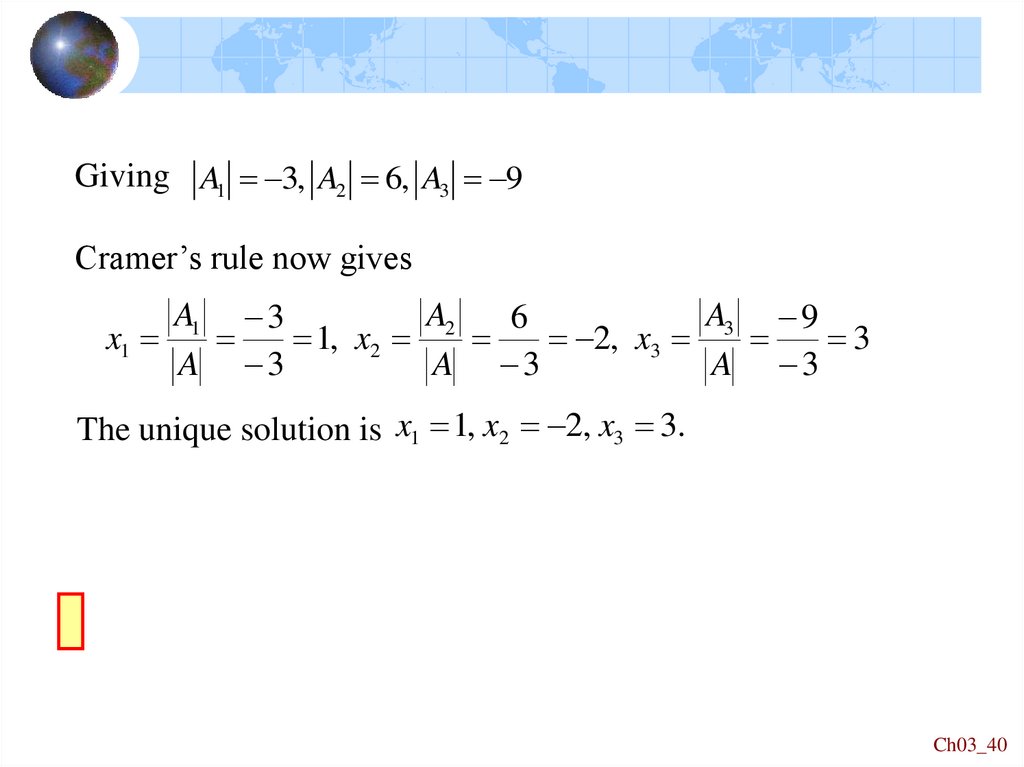
40.

Giving A1 3, A2 6, A3 9
Cramer’s rule now gives
A1 3
A2
A3 9
6
x1
1, x2
2, x3
3
A 3
A 3
A 3
The unique solution is x1 1, x2 2, x3 3.
Ch03_40

41. Example 6

Determine values of for which the following system of
equations has nontrivial solutions.Find the solutions for each
value of .
( 2 ) x ( 4) x 0
1
2
2 x1 ( 1) x2 0
Solution
homogeneous system
x1 = 0, x2 = 0 is the trivial solution.
nontrivial solutions exist many solutions
2 4
0
2 1
( 2)( 1) 2( 4) 0 2 6 0 ( 2)( 3) 0
= – 3 or = 2.
Ch03_41

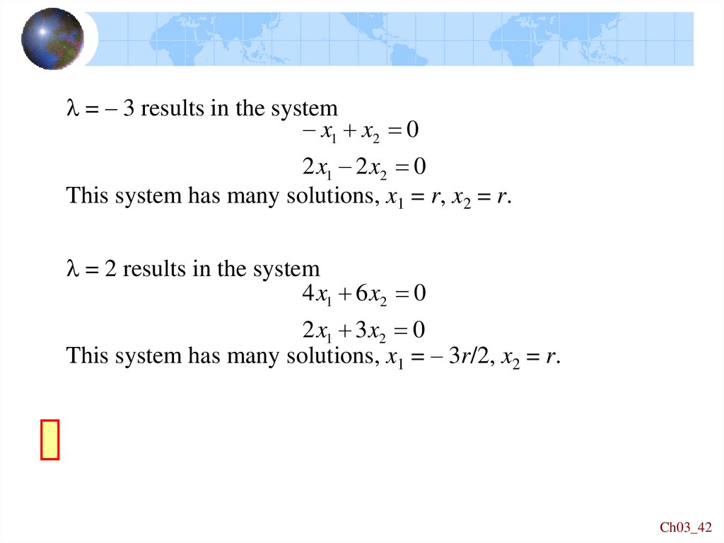
42.

= – 3 results in the system
x1 x2 0
2 x1 2 x2 0
This system has many solutions, x1 = r, x2 = r.
= 2 results in the system
4 x1 6 x2 0
2 x1 3 x2 0
This system has many solutions, x1 = – 3r/2, x2 = r.
Ch03_42

43. Homework

Exercises will be given by the teachers of
the practical classes.
Ch03_43