


 mathematics
Similar presentations:


Linear Algebra. Chapter 1. Linear Equations in Linear Algebra
1. Chapter 1 Linear Equations in Linear Algebra
Linear AlgebraChapter 1
Linear Equations in Linear
Algebra
2. 1.1 Matrices and Systems of Linear Equations
Definition• An equation such as x+3y=9 is called a linear equation
(in two variables or unknowns).
• The graph of this equation is a straight line in the xy-plane.
• A pair of values of x and y that satisfy the equation is called
a solution.
Ch1_2
3.
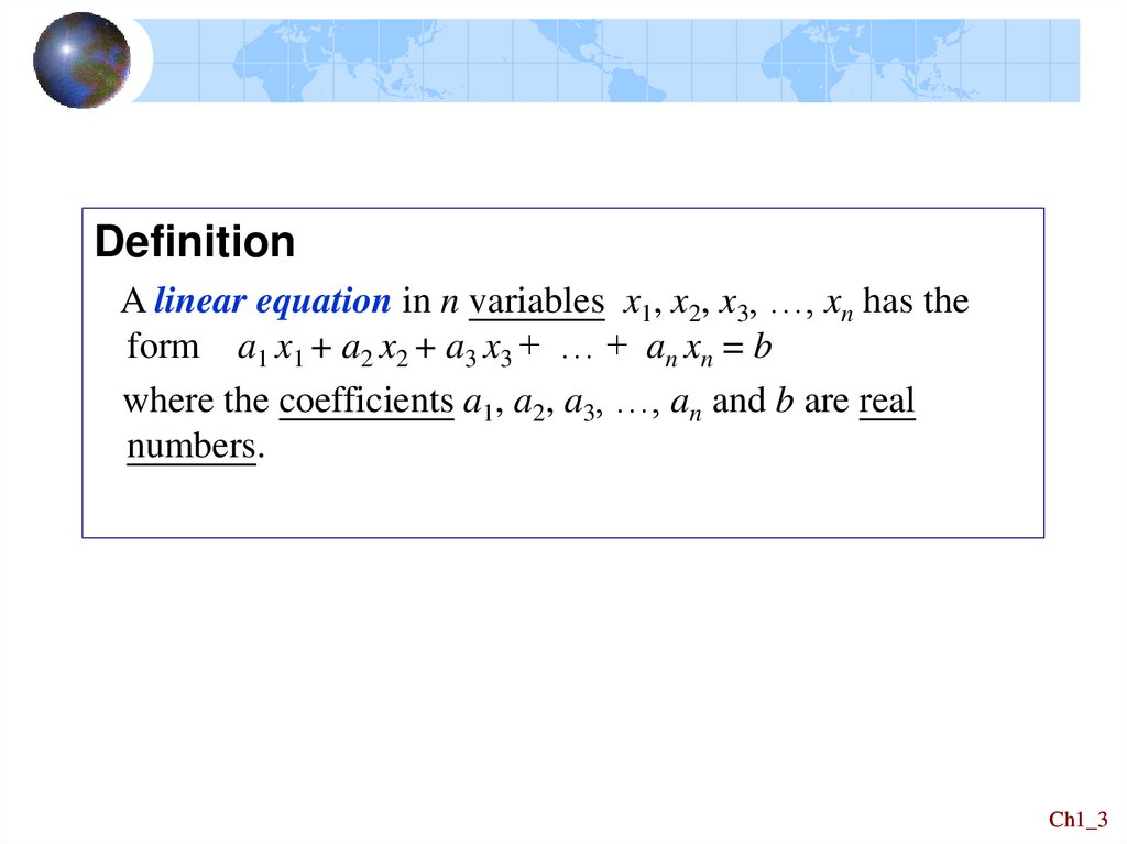
DefinitionA linear equation in n variables x1, x2, x3, …, xn has the
form a1 x1 + a2 x2 + a3 x3 + … + an xn = b
where the coefficients a1, a2, a3, …, an and b are real
numbers.
Ch1_3
4. Solutions for system of linear equations
Figure 1.1Unique solution
x + 3y = 9
–2x + y = –4
Lines intersect at (3, 2)
Unique solution:
x = 3, y = 2.
Figure 1.2
No solution
–2x + y = 3
–4x + 2y = 2
Lines are parallel.
No point of intersection.
No solutions.
Figure 1.3
Many solution
4x – 2y = 6
6x – 3y = 9
Both equations have the
same graph. Any point on
the graph is a solution.
Many solutions.
Ch1_4
5.
A linear equation in three variables corresponds toa plane in three-dimensional space.
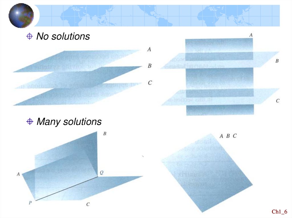
※ Systems of three linear equations in three variables:
Unique solution
Ch1_5
6.
No solutionsMany solutions
Ch1_6
7.
A solution to a system of a three linear equations will bepoints that lie on all three planes.
The following is an example of a system of three linear
equations:
x1
x2
x3 2
2 x1 3 x2
x3 3
x1 x2 2 x3 6
How to solve a system of linear equations? For this we
introduce a method called Gauss-Jordan elimination.
(Section1.2)
Ch1_7
8.
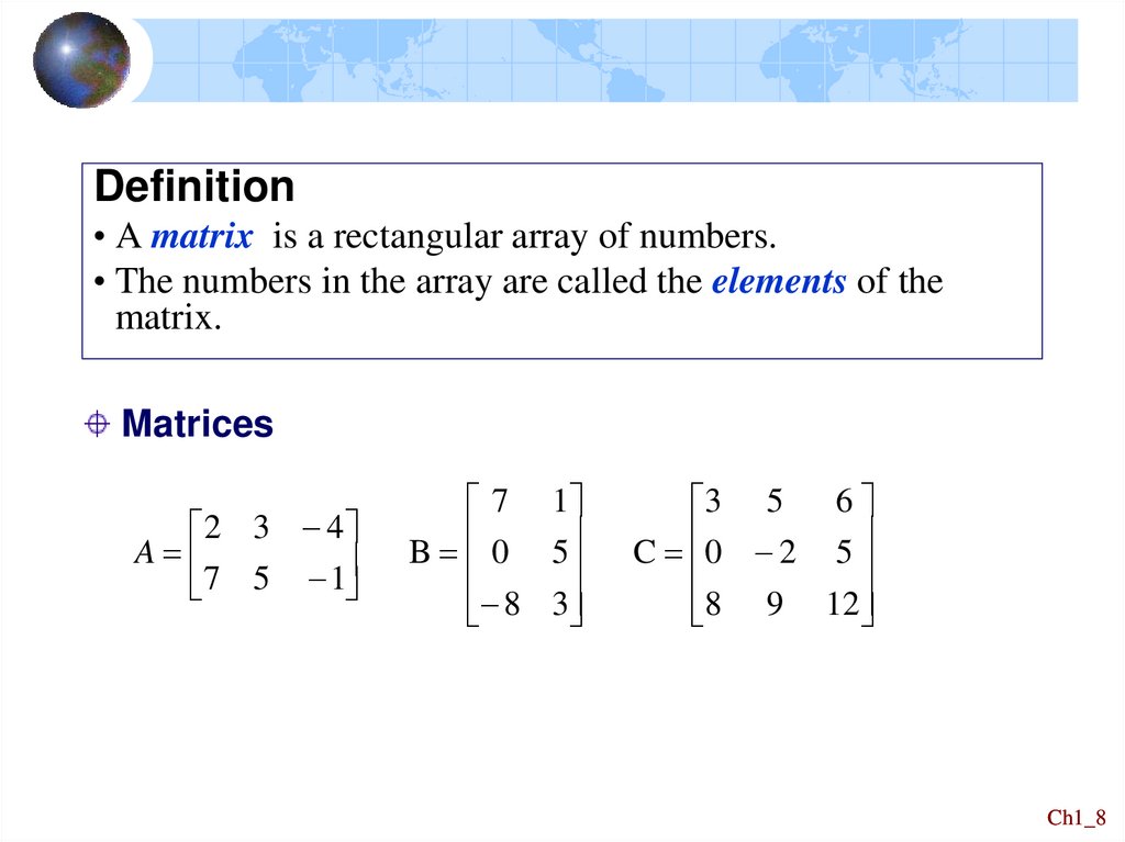
Definition• A matrix is a rectangular array of numbers.
• The numbers in the array are called the elements of the
matrix.
Matrices
2 3 4
A
7
5
1
7 1
B 0 5
8 3
6
3 5
C 0 2 5
8 9 12
Ch1_8
9.
2 3 4A
7
5
1
Row and Column
2 3 4
7 5 1
row 1
row 2
2
7
column 1
3
5
column 2
4
1
column 3
Submatrix
1 7 4
A 2 3 0
5 1 2
matrix A
1 7
P 2 3
5 1
7
4
1
Q 3
R
5
2
1
submatrice s of A
Ch1_9
10.
Size and Type1 0
2 4
2 5 7
9 0 1
3 5 8
3 3 matrix
3
5
Size : 2 3
1 4 matrix
8
3
2
3 1 matrix
a row matrix
a column matrix
4
a square matrix
3 8
5
Location
2 3 4
A
7 5 1
a13 4, a21 7
The element aij is in row i , column j
The element in location (1,3) is 4
Identity Matrices
diagonal size
I 2 1 0
0 1
1 0 0
I 3 0 1 0
0 0 1
Ch1_10
11.
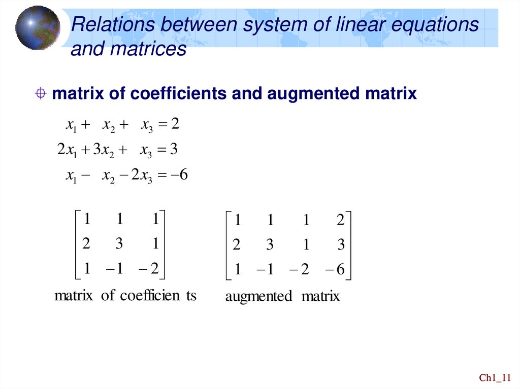
Relations between system of linear equationsand matrices
matrix of coefficients and augmented matrix
x1 x2 x3 2
2 x1 3x2 x3 3
x1 x2 2 x3 6
1
1 1
2
3
1
1 1 2
matrix of coefficien ts
1
2
1 1
2
3
1
3
1 1 2 6
augmented matrix
Ch1_11
12.
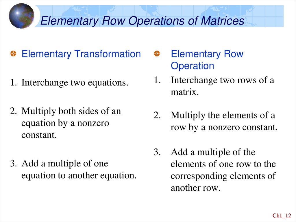
Elementary Row Operations of MatricesElementary Transformation
1. Interchange two equations.
2. Multiply both sides of an
equation by a nonzero
constant.
3. Add a multiple of one
equation to another equation.
Elementary Row
Operation
1. Interchange two rows of a
matrix.
2.
Multiply the elements of a
row by a nonzero constant.
3.
Add a multiple of the
elements of one row to the
corresponding elements of
another row.
Ch1_12
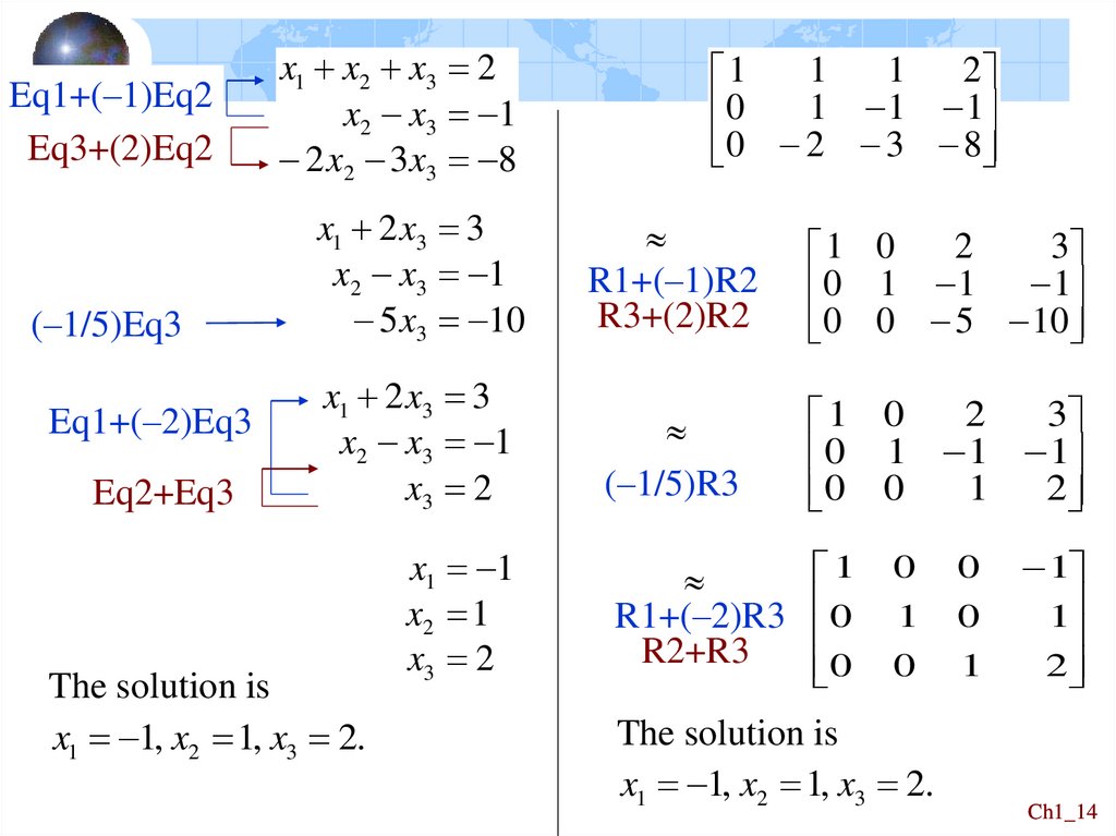
13. Example 1
Solving the following system of linear equation.x1 x2 x3 2
2 x1 3 x2 x3 3
x1 x2 2 x3 6
row equivalent
Solution
Equation Method
Initial system:
x1 x2 x3 2
Eq2+(–2)Eq1
2 x1 3 x2 x3 3
x1 x2 2 x3 6
Eq3+(–1)Eq1
x1 x2 x3 2
Analogous Matrix Method
Augmented matrix:
1
2
1 1
3
1
3
2
1 1 2 6
x2 x3 1 R2+(–2)R1
2 x2 3x3 8 R3+(–1)R1
1
1
2
1
1 1 1
0
0 2 3 8
Ch1_13
14.
Eq1+(–1)Eq2Eq3+(2)Eq2
x1 x2 x3 2
x2 x3 1
2 x2 3 x3 8
(–1/5)Eq3
x1 2 x3 3
x2 x3 1
5 x3 10
R1+(–1)R2
R3+(2)R2
2
3
1 0
0 1 1 1
0 0 5 10
x1 2 x3 3
x2 x3 1
x3 2
(–1/5)R3
2
3
1 0
0 1 1 1
1
2
0 0
R1+(–2)R3
R2+R3
1
0
0
Eq1+(–2)Eq3
Eq2+Eq3
The solution is
x1 1, x2 1, x3 2.
x1 1
x2 1
x3 2
1
1
2
1
1 1 1
0
0 2 3 8
0
0
1
0
0
1
The solution is
x1 1, x2 1, x3 2.
1
1
2
Ch1_14
15. Example 2
Solving the following system of linear equation.x1 2 x2 4 x3 12
2 x1 x2 5 x3 18
x1 3 x2 3 x3 8
Solution
4 12
4 12
1 2
1 2
R2 ( 2)R1
5 18
3 3 6
2 1
0
R3 R1
3 3 8
1
1
4
1
0
1
R2
3
1 2 4 12
1 1 2
0
1 1
4
0
R1 (2)R2
R3 ( 1) R2
8
1 0 2
0 1 1 2
6
0 0 2
8
1 0 2
1 0 0 2
0 1 1 2 R1 ( 2)R3
0
1
0
1
1
R2 R3
R3
0 0
1
3
0 0 1 3
2
x1 2
solution x2 1.
x 3
3
Ch1_15
16. Example 3
Solve the system4 x1 8 x2 12 x3 44
3 x1 6 x2 8 x3 32
2 x1 x2
7
Solution
1 2 3 11
4 8 12 44
1 2 3 11
3 6 8 32 R2 ( 3)R1
3 6 8 32
0
0
1
1
1 R1
R3
2
R1
2 1
0 7
0 7 4
0 3 6 15
2 1
1 2 3 11
1 2 3 11
0 1 2
0 3 6 15
5
R2 R3
R1 ( 2)R2
1 R2
0 0
0 0
1 1
1 1 3
1 0 0
R1 ( 1)R3
R2 2R3
2
0 1 0
.
3
0 0 1 1
1 1
1 0
0 1 2
5
0 0
1 1
The solution is x1 2, x2 3, x3 1.
Ch1_16
17. Summary
8 12 444
[ A : B ] 3 6 8 32
2 1
0 7
4 x1 8 x2 12 x3 44
3 x1 6 x2 8 x3 32
2 x1 x2
7
A
Use row operations to [A: B] :
1
8 12 44
4
3 6 8 32 0
2 1
0 7
0
0
0
1
0
0
1
2
3 .
1
B
i.e., [ A : B] [ I n : X ]
Def. [In : X] is called the reduced echelon form of [A : B].
Note. 1. If A is the matrix of coefficients of a system of n equations
in n variables that has a unique solution,
then A is row equivalent to In (A In).
2. If A In, then the system has unique solution.
Ch1_17
18. Example 4 Many Systems
Solving the following three systems of linear equation, all ofwhich have the same matrix of coefficients.
x1 x2 3 x3 b1
b1 8 0 3
2 x1 x2 4 x3 b2 for b2 11 , 1 , 3 in turn
b 11 2 4
x1 2 x2 4 x3 b3
3
Solution
3
8 0
3
3
8 0
3
1 1
1 1
4
11 1
3 R2+(–2)R1 0
1 2 5 1 3
2 1
R3+R1
1 1 3 2 1
1 2 4 11 2 4
0
1 0
1
3 1
0
1 0 0 1 0 2
0 1 2 5 1 3 R1 ( 1) R3
R1 R2
0 1 0 1 3
1
R3 ( 1)R2
0 0
R2 2 R3
1
2
1
2
2 1
2
0 0 1
x1 1 x1 0 x1 2
The solutions to
x
1
,
x
3
,
2
x2 1 .
the three systems are 2
x 2 x 1 x 2
3
3
3
Ch1_18
19. Homework
Exercises will be given by the teachers ofthe practical classes.
Ch1_19
20. 1.2 Gauss-Jordan Elimination
DefinitionA matrix is in reduced echelon form if
1. Any rows consisting entirely of zeros are grouped at the
bottom of the matrix.
2. The first nonzero element of each other row is 1. This
element is called a leading 1.
3. The leading 1 of each row after the first is positioned to
the right of the leading 1 of the previous row.
4. All other elements in a column that contains a leading 1
are zero.
Ch1_20
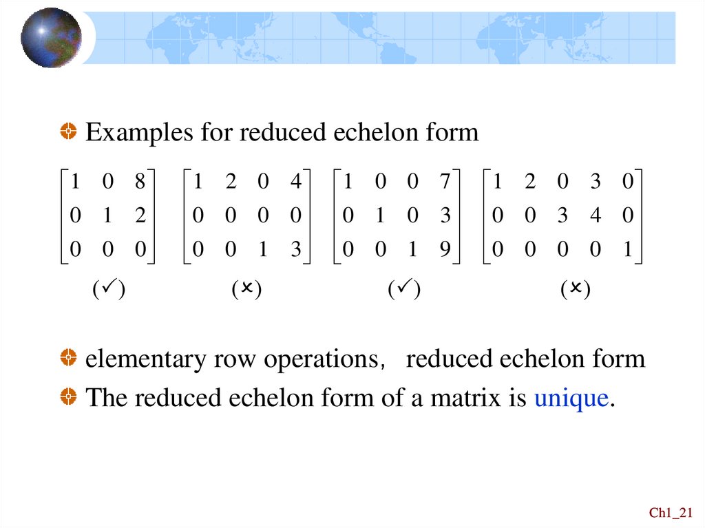
21.
Examples for reduced echelon form1 0 8
0 1 2
0 0 0
( )
1 2 0 4
0 0 0 0
0 0 1 3
( )
1 0 0 7
0 1 0 3
0 0 1 9
( )
1 2 0 3 0
0 0 3 4 0
0 0 0 0 1
( )
elementary row operations reduced echelon form
The reduced echelon form of a matrix is unique.
Ch1_21
22. Gauss-Jordan Elimination
System of linear equationsaugmented matrix
reduced echelon form
solution
Ch1_22
23. Example 1
Use the method of Gauss-Jordan elimination to find reducedechelon form of the following matrix.
2 2 2
0 0
9 12
3 3 3
4 4 2 11 12
pivot (leading 1)
Solution
3
3 3
9 12 1 1 1
3 4
2 2 2
0
2 2
2 1 R1 0 0
0
R1 R2
4 4 2 11 12
3
4
4
2
11
12
1 1 1
2
0 0
R3 ( 4)R1
0 0
pivot 2
3
2
1
1
1
2 R2 0
2
4
0
4
1
1
3
0
1
1
0
2
1
4
1
4
5
1 1 0 2
1 1 0 0 17
R1 R2 0 0 1 1
1 R1 ( 2)R3 0 0 1 0 5
R3 ( 2)R2 0 0 0
1 6 R2 R3 0 0 0 1 6
The matrix is the reduced echelon form of the given matrix.
Ch1_23
24. Example 2
Solve, if possible, the system of equations3 x1 3 x2 3 x3 9
2 x1 x2 4 x3 7
3 x1 5 x2 x3 7
Solution
1
3
3 3 3 9 1 1 1 3 1 1
1
2
1
2 1 4 7 1 R1 2 1 4 7 R2 ( 2)R1 0
3 5 1 7 3 3 5 1 7 R3 ( 3)R1 0 2 4 2
1 0 3 4
R1 R2 0
1 2 1
0 0 0 0
x 3 x3 4 x1 3 x3 4
1
x2 2 x3 1 x2 2 x3 1
R3 2R2
The general solution to the system is
x1 3r 4
x2 2r 1
x3 r
, where r is real number (called a parameter) .
Ch1_24
25. Example 3
Solve the system of equations2 x1 4 x2 12 x3 10 x4 58
x1 2 x2 3 x3 2 x4 14
2 x1 4 x2 9 x3 6 x4 44
Solution
2 4 12
2 3
1
9
2 4
1 2
R2 R1 0
0
R3 ( 2)R1
0
0
1 2
R1 ( 6)R2 0
0
R3 3R2
0
0
many sol.
10
58 1 2
6 5
29
2 14 1 R1 1
2 3
2 14
6
44 2 2 4
9 6
44
6 5
29 1 2
6 5
29
3 3
15 1 R2 0
0
1 1
5
3
4 14 3 0
0 3
4 14
0
1 1 1 2 0 0 2
1 1 5 R1 ( 1)R3 0
0 1 0
6
0
1 1 R2 R3 0
0 0 1
1
x1 2 x2 2
x3 6
x4 1
x1 2r 2
x2 r
, for some r.
x3 6
x4 1
Ch1_25
26. Example 4
Solve the system of equationsx1 2 x2 x3 3 x4 x5 2
2 x1 4 x2 2 x3 6 x4 3 x5 6
x1 2 x2 x3 x4 3 x5 4
Solution
2 1 3 1 2 1 2 1 3 1 2
1
4 2 6 3 6 R2 ( 2)R1 0 0 0 0 1 2
2
1 1 3 4 R3 R1 0 0 0 2 4 6
1 2
1 2 1 3 1 2 1 2 1 3 1 2
0 0 0 2 4 6
0 0 0 1 2 3
1
R
2
R2 R3
0 0 0 0 1 2 2 0 0 0 0 1 2
1 2 1 0 5 7
1 2 1 0 0
3
0 0 0 1
2
3 R1 5R3 0 0 0 1 0 1
R1 ( 3)R2
1
2 R2 ( 2)R3 0 0 0 0 1 2
0 0 0 0
x1 2r s 3
x1 2 x2 x3 3
x4 1
x2 r , x3 s, x4 1, , for some r and s.
x5 2
x5 2
Ch1_26
27. Example 5
This example illustrates a system that has no solution. Let us tryto solve the system
x1 x2 2 x3 3
2 x1 2 x2 5 x3 4
x1 2 x2 x3 3
2 x2 2 x3 1
Solution
1 1 2 3 1 1 2 3
1 1 2 3
2 2 5 4 R2 ( 2)R1 0 0 1 2 0 3 3 6
1 2 1 3 R3 ( 1)R1 0 3 3 6 R2 R3 0 0 1 2
0 2 2 1
0 2 2 1
0 2 2 1
1
0 0
3
1 1 2 3 1 0 1 1
0
1
0
4
0 1 1 2
0 1 1 2 R1 ( 1)R3
R1 R2
1
R2
R3
3 R2 0 0 1 2 R4 ( 2)R2 0 0 1 2 R4 ( 4)R3 0 0 1 2
0 2 2 1
0 0 4 5
0
0 0 13
1 0 0 3
0x1+0x2+0x3=1
0 1 0 4
131 R4 0 0 1 2 The system has no solution.
0 0 0 1
Ch1_27
28. Homogeneous System of linear Equations
DefinitionA system of linear equations is said to be homogeneous if all
the constant terms are zeros.
Example:
x1 2 x2 5 x3 0
2 x1 3 x2 6 x3 0
Observe that x1 0, x2 0, x3 0 is a solution.
Theorem 1.1
A system of homogeneous linear equations in n variables always
has the solution x1 = 0, x2 = 0. …, xn = 0. This solution is called
the trivial solution.
Ch1_28
29. Homogeneous System of linear Equations
Note. Non trivial solutionExample: x1 2 x2 5 x3 0
2 x1 3 x2 6 x3 0
The system has other nontrivial solutions.
2 5 0
1
1 0 3 0
2 3 6 0 0 1 4 0
x1 3r , x2 4r , x3 r
Theorem 1.2
A system of homogeneous linear equations that has more
variables than equations has many solutions.
Ch1_29
30. Homework
Exercise will be given by the teachers of thepractical classes.
Ch1_30
31. 1.3 Gaussian Elimination
DefinitionA matrix is in echelon form if
1. Any rows consisting entirely of zeros are
grouped at the bottom of the matrix.
2. The first nonzero element of each row is 1. This
element is called a leading 1.
3. The leading 1 of each row after the first is
positioned to the right of the leading 1 of the
previous row.
(This implies that all the elements below a leading 1
are zero.)
Ch1_31
32.
Example 6Solving the following system of linear equations using the
method of Gaussian elimination.
x1 2 x2 3 x3 2 x4 1
x1 2 x2 2 x3 x4 2
2 x1 4 x2 8 x3 12 x4 4
Solution
Starting with the augmented matrix, create zeros below the pivot
in the first column.
2
3 2 1
1
1 2 3 2 1
1 2 2 1 2 R 2 R1 0 0 1 3
1
2
4
8 12 4 R3 ( 2) R1 0 0 2 8 6
At this stage, we create a zero only below the pivot.
1 2 3 2 1 1 2 3 2 1
0 0 1 3
1 1 0 0 1 3
1
R3
R3 ( 2) R 2
2
0 0 0 2 4
0 0 0 1 2
Echelon form
We have arrived at the echelon form.
Ch1_32
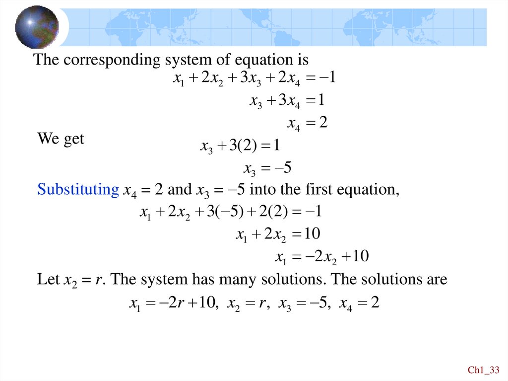
33.
The corresponding system of equation isx1 2 x2 3x3 2 x4 1
x3 3x4 1
x4 2
We get
x3 3(2) 1
x3 5
Substituting x4 = 2 and x3 = 5 into the first equation,
x1 2 x2 3( 5) 2(2) 1
x1 2 x2 10
x1 2 x2 10
Let x2 = r. The system has many solutions. The solutions are
x1 2r 10, x2 r , x3 5, x4 2
Ch1_33
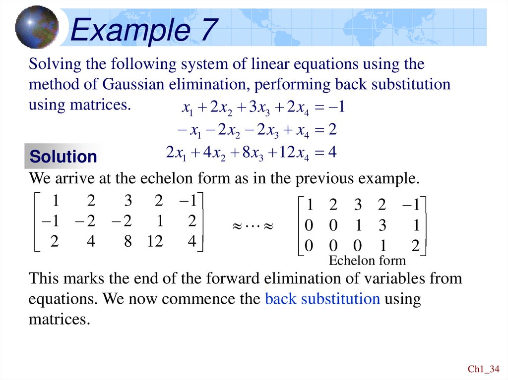
34.
Example 7Solving the following system of linear equations using the
method of Gaussian elimination, performing back substitution
using matrices.
x1 2 x2 3 x3 2 x4 1
x1 2 x2 2 x3 x4 2
2 x1 4 x2 8 x3 12 x4 4
Solution
We arrive at the echelon form as in the previous example.
2
3 2 1
1
1 2 3 2 1
1 2 2 1 2
0 0 1 3
1
2
0 0 0 1 2
4
8 12 4
Echelon form
This marks the end of the forward elimination of variables from
equations. We now commence the back substitution using
matrices.
Ch1_34
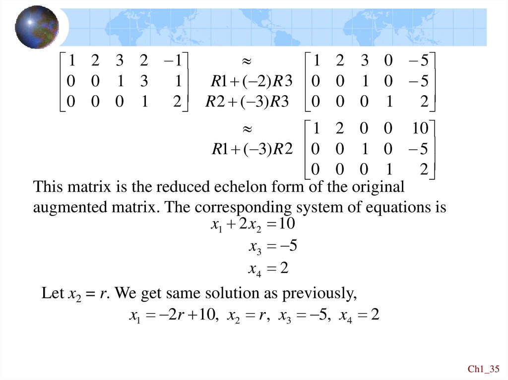
35.
1 2 3 2 10 0 1 3
1
0 0 0 1 2
1 2 3 0 5
R1 ( 2) R 3 0 0 1 0 5
R 2 ( 3) R3 0 0 0 1
2
1 2 0 0 10
R1 ( 3) R 2 0 0 1 0 5
0 0 0 1
2
This matrix is the reduced echelon form of the original
augmented matrix. The corresponding system of equations is
x1 2 x2 10
x3 5
x4 2
Let x2 = r. We get same solution as previously,
x1 2r 10, x2 r , x3 5, x4 2
Ch1_35