Spreadsheet MS Excel. Engineering and technological calculations tasks in Microsoft Excel spreadsheet

1.

Theme: Spreadsheet MS Excel.
Engineering and technological
calculations tasks in Microsoft Excel
spreadsheet
Тема: ЭТ MS Excel. Решение
инженерные и технологических
задач в Microsoft Excel

2.

Microsoft Office Excel is a powerful
program which used to create engineering and
technological calculations of many different tasks.
Spreadsheet MS Excel has some facility for
solving this problems. Main capabilities in
Spreadsheet MS Excel are the functions and the
diagrams masters.

3.

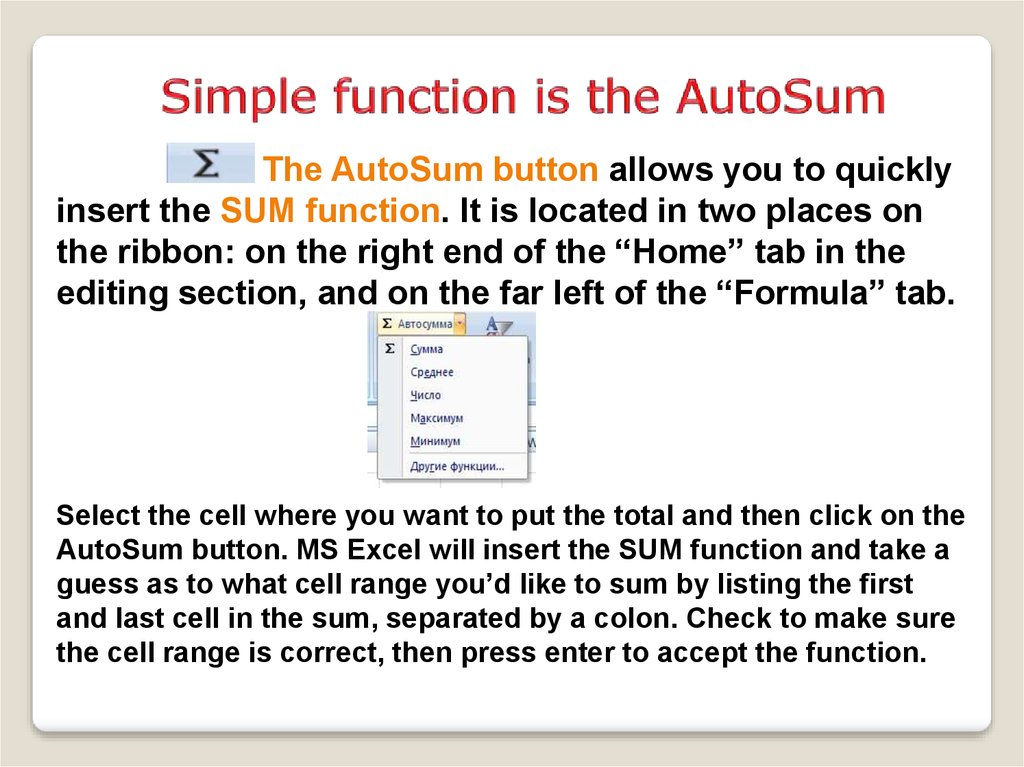
The AutoSum button allows you to quickly
insert the SUM function. It is located in two places on
the ribbon: on the right end of the “Home” tab in the
editing section, and on the far left of the “Formula” tab.
Select the cell where you want to put the total and then click on the
AutoSum button. MS Excel will insert the SUM function and take a
guess as to what cell range you’d like to sum by listing the first
and last cell in the sum, separated by a colon. Check to make sure
the cell range is correct, then press enter to accept the function.

4.

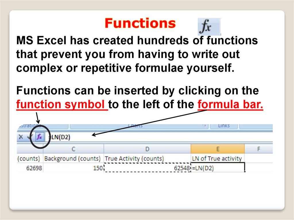
MS Excel has created hundreds of functions
that prevent you from having to write out
complex or repetitive formulae yourself.
Functions can be inserted by clicking on the
function symbol to the left of the formula bar.

5.

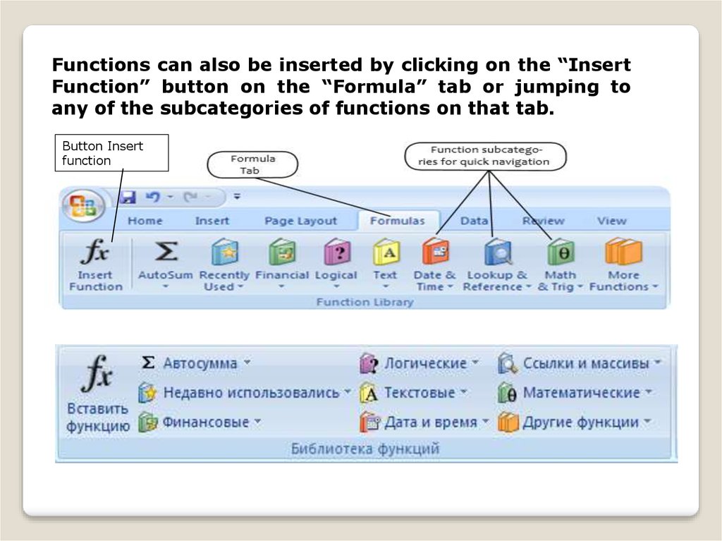
Functions can also be inserted by clicking on the “Insert
Function” button on the “Formula” tab or jumping to
any of the subcategories of functions on that tab.
Button Insert
function

6.

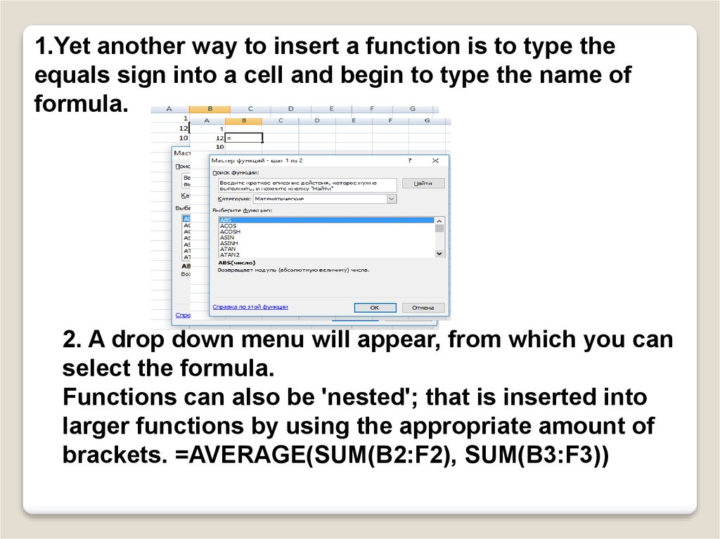
1.Yet another way to insert a function is to type the
equals sign into a cell and begin to type the name of
formula.
2. A drop down menu will appear, from which you can
select the formula.
Functions can also be 'nested'; that is inserted into
larger functions by using the appropriate amount of
brackets. =AVERAGE(SUM(B2:F2), SUM(B3:F3))

7.

Accessing MS Excel functions
Worksheet
functions
are
categorized
by
their
functionality. Click a category to browse its functions.
Or press Ctrl+F to find a function by typing the first few
letters or a descriptive word. To get detailed information
about a function, click its name in the first column.
Statistical functions:
SUM: Adds a range of cells
together
AVERAGE: Calculates the
average of a range of cells
COUNT: Counts the number
of chosen data in a range of
cells
MAX: Identifies the largest
number in a range of cells
MIN: Identifies the smallest
number in a range of cells
Financial functions:
Interest rates
Loan payments
Depreciation amounts

8.

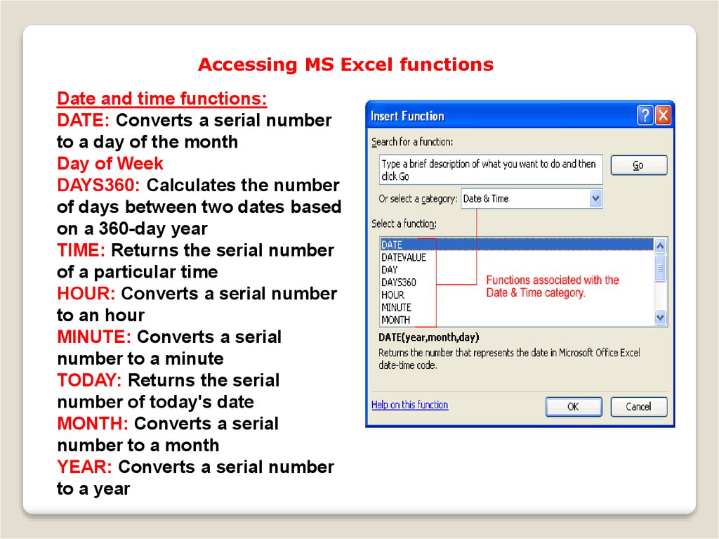
Accessing MS Excel functions
Date and time functions:
DATE: Converts a serial number
to a day of the month
Day of Week
DAYS360: Calculates the number
of days between two dates based
on a 360-day year
TIME: Returns the serial number
of a particular time
HOUR: Converts a serial number
to an hour
MINUTE: Converts a serial
number to a minute
TODAY: Returns the serial
number of today's date
MONTH: Converts a serial
number to a month
YEAR: Converts a serial number
to a year

9.

The parts of a function:
Each function has a specific order, called syntax,
which must be strictly followed for the function to
work correctly.
Syntax order:
1.All functions begin with the = sign.
2.After the = sign, define the function name (e.g.,
Sum).
3.Then there will be an argument. An argument is
the cell range or cell references that are enclosed
by parentheses. If there is more than one
argument, separate each by a comma.
An example of a function with one argument that
adds a range of cells, A3 through A9:

10.

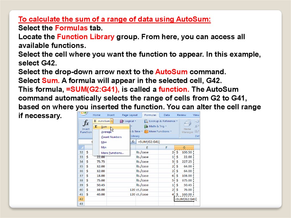
To calculate the sum of a range of data using AutoSum:
Select the Formulas tab.
Locate the Function Library group. From here, you can access all
available functions.
Select the cell where you want the function to appear. In this example,
select G42.
Select the drop-down arrow next to the AutoSum command.
Select Sum. A formula will appear in the selected cell, G42.
This formula, =SUM(G2:G41), is called a function. The AutoSum
command automatically selects the range of cells from G2 to G41,
based on where you inserted the function. You can alter the cell range
if necessary.

11.

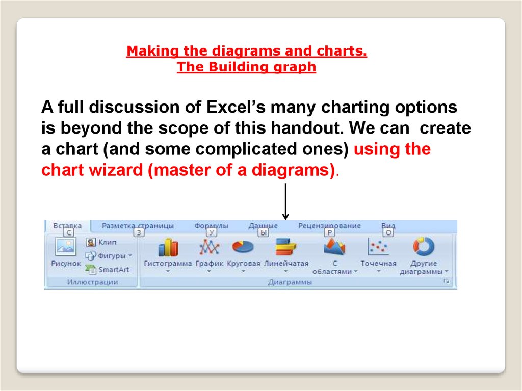
Making the diagrams and charts.
The Building graph
A full discussion of Excel’s many charting options
is beyond the scope of this handout. We can create
a chart (and some complicated ones) using the
chart wizard (master of a diagrams).

12.

Just highlight the data you wish to base your chart on
(including header rows, if you have any) and click on
the Insert tab and you will see the available charts
there. When you click on a type of chart, you will be
prompted to select a subtype of chart. Once you have
done so, the chart will appear on your spreadsheet.
Three additional tabs will also appear on your ribbon ,
through which you can alter your chart by adding
titles, changing data points, and many other options.

13.

For
graphing
functions must
the
table
importance's
argument and
Choose
the
column.
of
the
to create
with
of
the
functions.
necessary
And then in master of the
diagrams to choose the
type of the diagram: point, but type – a graphic.