Similar presentations:
The Capital Asset Pricing Model (CAPM). Corporate Finance
1.
Chapter TenThe Capital Asset
Corporate Finance
Ross Westerfield Jaffe
Pricing Model (CAPM)
Prepared by
Gady Jacoby
University of Manitoba
and
Sebouh Aintablian
American University of
Beirut
10
Sixth Edition
2.
10.1 Individual Securities10.2 Expected Return, Variance, and Covariance
10.3 The Return and Risk for Portfolios
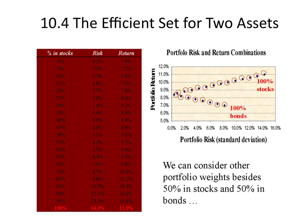
10.4 The Efficient Set for Two Assets
10.5 The Efficient Set for Many Securities
10.6 Diversification: An Example
10.7 Riskless Borrowing and Lending
10.8 Market Equilibrium
10.9 Relationship between Risk and Expected Return (CAPM)
10.10 Summary and Conclusions
3. 10.1 Individual Securities
• The characteristics of individual securities thatare of interest are the:
– Expected Return
– Variance and Standard Deviation
– Covariance and Correlation
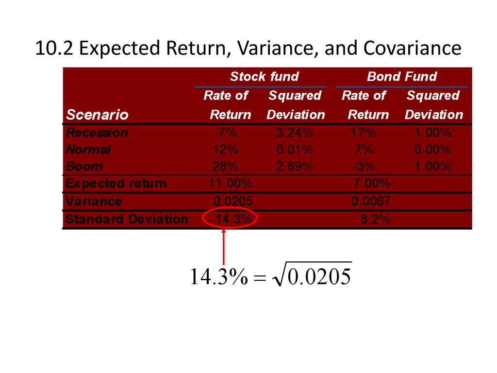
4. 10.2 Expected Return, Variance, and Covariance
Rate of ReturnScenario Probability Stock fund Bond fund
Recession
33.3%
-7%
17%
Normal
33.3%
12%
7%
Boom
33.3%
28%
-3%
Consider the following two risky asset
worlds. There is a 1/3 chance of each state of
the economy and the only assets are a stock
fund and a bond fund.
5. 10.2 Expected Return, Variance, and Covariance
ScenarioRecession
Normal
Boom
Expected return
Variance
Standard Deviation
Stock fund
Rate of
Squared
Return Deviation
-7%
3.24%
12%
0.01%
28%
2.89%
11.00%
0.0205
14.3%
Bond Fund
Rate of
Squared
Return Deviation
17%
1.00%
7%
0.00%
-3%
1.00%
7.00%
0.0067
8.2%
6. 10.2 Expected Return, Variance, and Covariance
ScenarioRecession
Normal
Boom
Expected return
Variance
Standard Deviation
Stock fund
Rate of
Squared
Return Deviation
-7%
3.24%
12%
0.01%
28%
2.89%
11.00%
0.0205
14.3%
Bond Fund
Rate of
Squared
Return Deviation
17%
1.00%
7%
0.00%
-3%
1.00%
7.00%
0.0067
8.2%
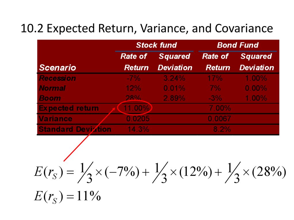
E (rS ) 1 ( 7%) 1 (12%) 1 (28%)
3
3
3
E (rS ) 11 %
7. 10.2 Expected Return, Variance, and Covariance
ScenarioRecession
Normal
Boom
Expected return
Variance
Standard Deviation
Stock fund
Rate of
Squared
Return Deviation
-7%
3.24%
12%
0.01%
28%
2.89%
11.00%
0.0205
14.3%
Bond Fund
Rate of
Squared
Return Deviation
17%
1.00%
7%
0.00%
-3%
1.00%
7.00%
0.0067
8.2%
E (rB ) 1 (17%) 1 (7%) 1 ( 3%)
3
3
3
E (rB ) 7%
8. 10.2 Expected Return, Variance, and Covariance
ScenarioRecession
Normal
Boom
Expected return
Variance
Standard Deviation
Stock fund
Rate of
Squared
Return Deviation
-7%
3.24%
12%
0.01%
28%
2.89%
11.00%
0.0205
14.3%
Bond Fund
Rate of
Squared
Return Deviation
17%
1.00%
7%
0.00%
-3%
1.00%
7.00%
0.0067
8.2%
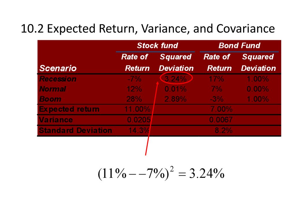
(11 % 7%) 3.24%
2
9. 10.2 Expected Return, Variance, and Covariance
ScenarioRecession
Normal
Boom
Expected return
Variance
Standard Deviation
Stock fund
Rate of
Squared
Return Deviation
-7%
3.24%
12%
0.01%
28%
2.89%
11.00%
0.0205
14.3%
Bond Fund
Rate of
Squared
Return Deviation
17%
1.00%
7%
0.00%
-3%
1.00%
7.00%
0.0067
8.2%
(11 % 12%) .01%
2
10. 10.2 Expected Return, Variance, and Covariance
ScenarioRecession
Normal
Boom
Expected return
Variance
Standard Deviation
Stock fund
Rate of
Squared
Return Deviation
-7%
3.24%
12%
0.01%
28%
2.89%
11.00%
0.0205
14.3%
Bond Fund
Rate of
Squared
Return Deviation
17%
1.00%
7%
0.00%
-3%
1.00%
7.00%
0.0067
8.2%
(11 % 28%) 2.89%
2
11. 10.2 Expected Return, Variance, and Covariance
ScenarioRecession
Normal
Boom
Expected return
Variance
Standard Deviation
Stock fund
Rate of
Squared
Return Deviation
-7%
3.24%
12%
0.01%
28%
2.89%
11.00%
0.0205
14.3%
Bond Fund
Rate of
Squared
Return Deviation
17%
1.00%
7%
0.00%
-3%
1.00%
7.00%
0.0067
8.2%
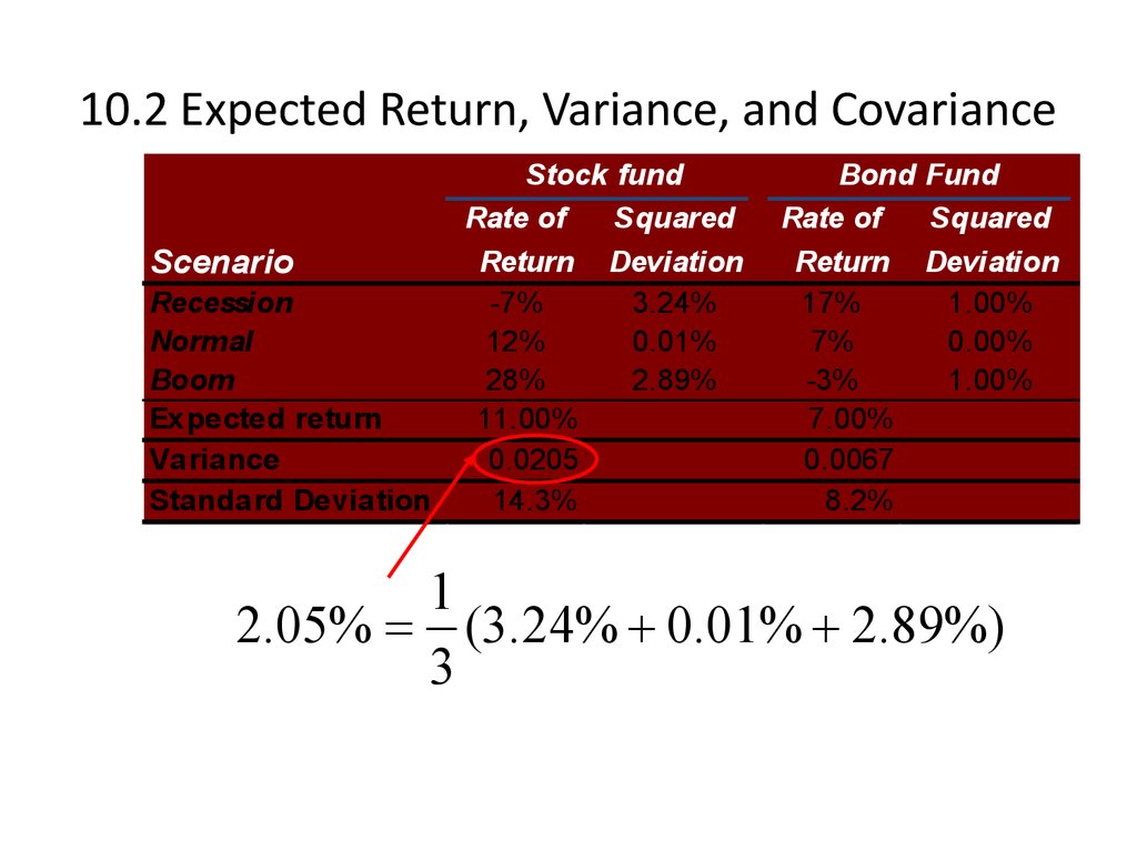
1
2.05% (3.24% 0.01% 2.89%)
3
12. 10.2 Expected Return, Variance, and Covariance
ScenarioRecession
Normal
Boom
Expected return
Variance
Standard Deviation
Stock fund
Rate of
Squared
Return Deviation
-7%
3.24%
12%
0.01%
28%
2.89%
11.00%
0.0205
14.3%
Bond Fund
Rate of
Squared
Return Deviation
17%
1.00%
7%
0.00%
-3%
1.00%
7.00%
0.0067
8.2%
14.3% 0.0205
13. 10.3 The Return and Risk for Portfolios
ScenarioRecession
Normal
Boom
Expected return
Variance
Standard Deviation
Stock fund
Rate of
Squared
Return Deviation
-7%
3.24%
12%
0.01%
28%
2.89%
11.00%
0.0205
14.3%
Bond Fund
Rate of
Squared
Return Deviation
17%
1.00%
7%
0.00%
-3%
1.00%
7.00%
0.0067
8.2%
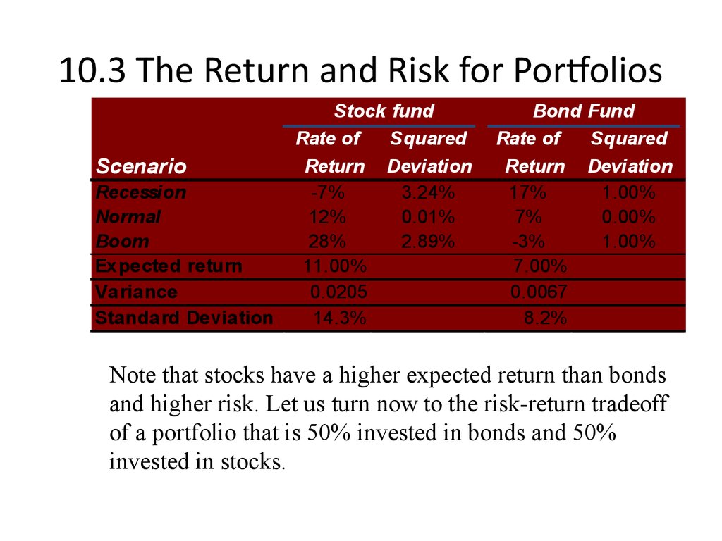
Note that stocks have a higher expected return than bonds
and higher risk. Let us turn now to the risk-return tradeoff
of a portfolio that is 50% invested in bonds and 50%
invested in stocks.
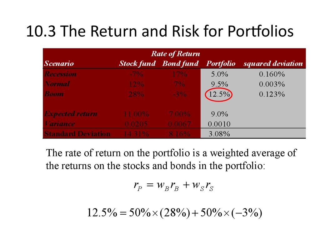
14. 10.3 The Return and Risk for Portfolios
Rate of ReturnStock fund Bond fund Portfolio
-7%
17%
5.0%
12%
7%
9.5%
28%
-3%
12.5%
Scenario
Recession
Normal
Boom
Expected return
Variance
Standard Deviation
11.00%
0.0205
14.31%
7.00%
0.0067
8.16%
squared deviation
0.160%
0.003%
0.123%
9.0%
0.0010
3.08%
The rate of return on the portfolio is a weighted average of
the returns on the stocks and bonds in the portfolio:
rP wB rB wS rS
5% 50% ( 7%) 50% (17%)
15. 10.3 The Return and Risk for Portfolios
Rate of ReturnStock fund Bond fund Portfolio
-7%
17%
5.0%
12%
7%
9.5%
28%
-3%
12.5%
Scenario
Recession
Normal
Boom
Expected return
Variance
Standard Deviation
11.00%
0.0205
14.31%
7.00%
0.0067
8.16%
squared deviation
0.160%
0.003%
0.123%
9.0%
0.0010
3.08%
The rate of return on the portfolio is a weighted average of
the returns on the stocks and bonds in the portfolio:
rP wB rB wS rS
9.5% 50% (12%) 50% (7%)
16. 10.3 The Return and Risk for Portfolios
Rate of ReturnStock fund Bond fund Portfolio
-7%
17%
5.0%
12%
7%
9.5%
28%
-3%
12.5%
Scenario
Recession
Normal
Boom
Expected return
Variance
Standard Deviation
11.00%
0.0205
14.31%
7.00%
0.0067
8.16%
squared deviation
0.160%
0.003%
0.123%
9.0%
0.0010
3.08%
The rate of return on the portfolio is a weighted average of
the returns on the stocks and bonds in the portfolio:
rP wB rB wS rS
12.5% 50% (28%) 50% ( 3%)
17. 10.3 The Return and Risk for Portfolios
Rate of ReturnStock fund Bond fund Portfolio
-7%
17%
5.0%
12%
7%
9.5%
28%
-3%
12.5%
Scenario
Recession
Normal
Boom
Expected return
Variance
Standard Deviation
11.00%
0.0205
14.31%
7.00%
0.0067
8.16%
squared deviation
0.160%
0.003%
0.123%
9.0%
0.0010
3.08%
The expected rate of return on the portfolio is a weighted
average of the expected returns on the securities in the
portfolio.
E (rP ) wB E (rB ) wS E (rS )
9% 50% (11 %) 50% (7%)
18. 10.3 The Return and Risk for Portfolios
ScenarioRecession
Normal
Boom
Expected return
Variance
Standard Deviation
Rate of Return
Stock fund Bond fund Portfolio
-7%
17%
5.0%
12%
7%
9.5%
28%
-3%
12.5%
11.00%
0.0205
14.31%
7.00%
0.0067
8.16%
squared deviation
0.160%
0.003%
0.123%
9.0%
0.0010
3.08%
The variance of the rate of return on the two risky assets
portfolio is
σ P2 (w B σ B ) 2 (wS σ S ) 2 2(w B σ B )(w S σ S )ρ BS
where BS is the correlation coefficient between the returns
on the stock and bond funds.
19. 10.3 The Return and Risk for Portfolios
ScenarioRecession
Normal
Boom
Expected return
Variance
Standard Deviation
Rate of Return
Stock fund Bond fund Portfolio
-7%
17%
5.0%
12%
7%
9.5%
28%
-3%
12.5%
11.00%
0.0205
14.31%
7.00%
0.0067
8.16%
squared deviation
0.160%
0.003%
0.123%
9.0%
0.0010
3.08%
Observe the decrease in risk that diversification offers.
An equally weighted portfolio (50% in stocks and 50%
in bonds) has less risk than stocks or bonds held in
isolation.
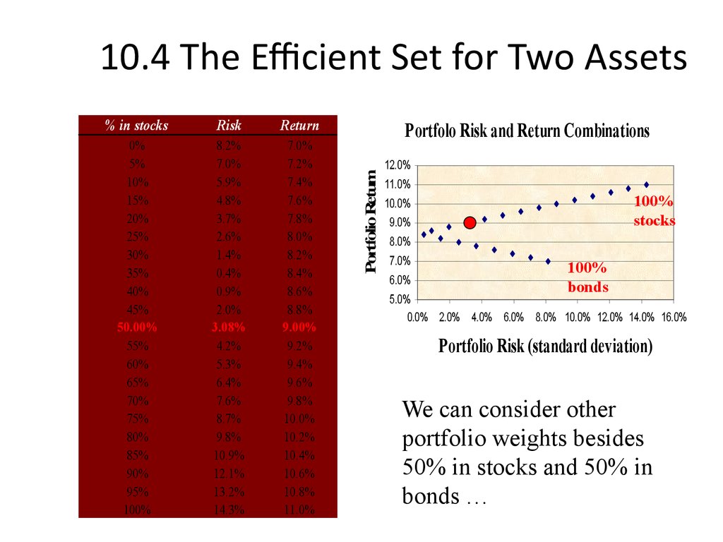
20. 10.4 The Efficient Set for Two Assets
RiskReturn
0%
5%
10%
15%
20%
25%
30%
35%
40%
45%
50.00%
55%
60%
65%
70%
75%
80%
85%
90%
95%
100%
8.2%
7.0%
5.9%
4.8%
3.7%
2.6%
1.4%
0.4%
0.9%
2.0%
3.08%
4.2%
5.3%
6.4%
7.6%
8.7%
9.8%
10.9%
12.1%
13.2%
14.3%
7.0%
7.2%
7.4%
7.6%
7.8%
8.0%
8.2%
8.4%
8.6%
8.8%
9.00%
9.2%
9.4%
9.6%
9.8%
10.0%
10.2%
10.4%
10.6%
10.8%
11.0%
Portfolo Risk and Return Combinations
Portfolio Return
% in stocks
12.0%
11.0%
100%
stocks
10.0%
9.0%
8.0%
7.0%
6.0%
100%
bonds
5.0%
0.0% 2.0% 4.0% 6.0% 8.0% 10.0% 12.0% 14.0% 16.0%
Portfolio Risk (standard deviation)
We can consider other
portfolio weights besides
50% in stocks and 50% in
bonds …
21. 10.4 The Efficient Set for Two Assets
RiskReturn
0%
0%
5%
5%
10%
10%
15%
15%
20%
20%
25%
25%
30%
30%
35%
35%
40%
40%
45%
45%
50%
50%
55%
55%
60%
60%
65%
65%
70%
70%
75%
75%
80%
80%
85%
85%
90%
90%
95%
95%
100%
100%
8.2%
8.2%
7.0%
7.0%
5.9%
5.9%
4.8%
4.8%
3.7%
3.7%
2.6%
2.6%
1.4%
1.4%
0.4%
0.4%
0.9%
0.9%
2.0%
2.0%
3.1%
3.1%
4.2%
4.2%
5.3%
5.3%
6.4%
6.4%
7.6%
7.6%
8.7%
8.7%
9.8%
9.8%
10.9%
10.9%
12.1%
12.1%
13.2%
13.2%
14.3%
14.3%
7.0%
7.0%
7.2%
7.2%
7.4%
7.4%
7.6%
7.6%
7.8%
7.8%
8.0%
8.0%
8.2%
8.2%
8.4%
8.4%
8.6%
8.6%
8.8%
8.8%
9.0%
9.0%
9.2%
9.2%
9.4%
9.4%
9.6%
9.6%
9.8%
9.8%
10.0%
10.0%
10.2%
10.2%
10.4%
10.4%
10.6%
10.6%
10.8%
10.8%
11.0%
11.0%
Portfolo Risk and Return Combinations
Portfolio Return
% in stocks
12.0%
11.0%
100%
stocks
10.0%
9.0%
8.0%
7.0%
6.0%
100%
bonds
5.0%
0.0% 2.0% 4.0% 6.0% 8.0% 10.0% 12.0% 14.0% 16.0%
Portfolio Risk (standard deviation)
We can consider other
portfolio weights besides
50% in stocks and 50% in
bonds …
22. 10.4 The Efficient Set for Two Assets
RiskReturn
0%
5%
10%
15%
20%
25%
30%
35%
40%
45%
50%
55%
60%
65%
70%
75%
80%
85%
90%
95%
100%
8.2%
7.0%
5.9%
4.8%
3.7%
2.6%
1.4%
0.4%
0.9%
2.0%
3.1%
4.2%
5.3%
6.4%
7.6%
8.7%
9.8%
10.9%
12.1%
13.2%
14.3%
7.0%
7.2%
7.4%
7.6%
7.8%
8.0%
8.2%
8.4%
8.6%
8.8%
9.0%
9.2%
9.4%
9.6%
9.8%
10.0%
10.2%
10.4%
10.6%
10.8%
11.0%
Portfolo Risk and Return Combinations
Portfolio Return
% in stocks
12.0%
11.0%
10.0%
100%
stocks
9.0%
8.0%
7.0%
6.0%
100%
bonds
5.0%
0.0% 2.0% 4.0% 6.0% 8.0% 10.0% 12.0% 14.0% 16.0%
Portfolio Risk (standard deviation)
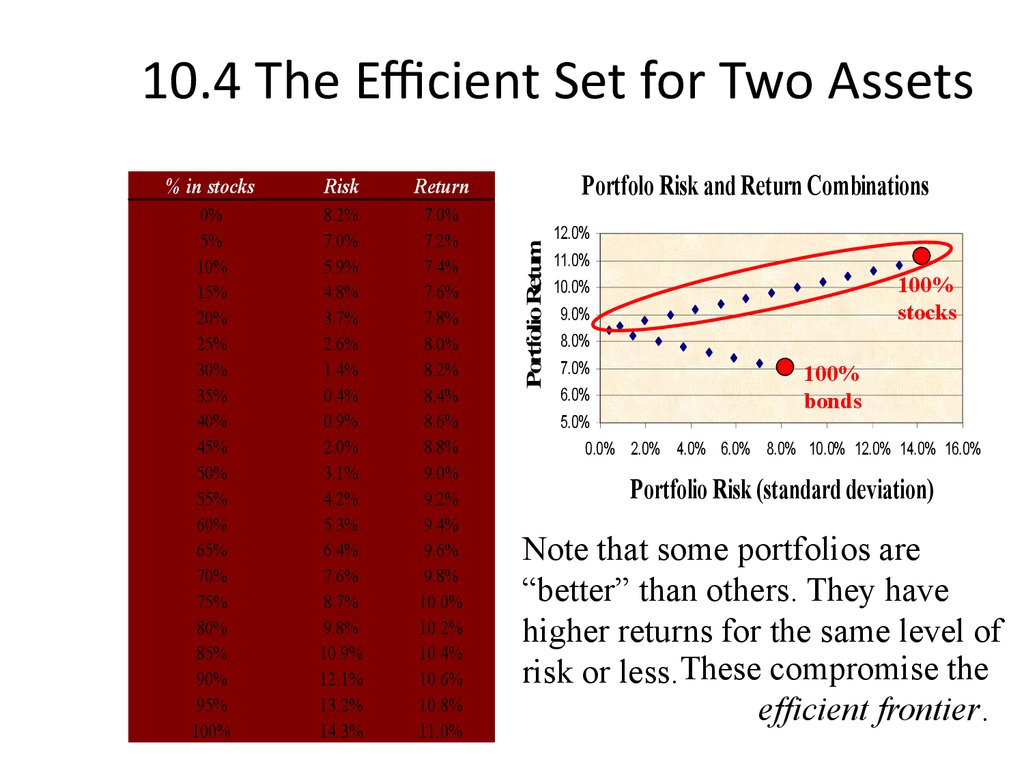
Note that some portfolios are
“better” than others. They have
higher returns for the same level of
risk or less. These compromise the
efficient frontier.
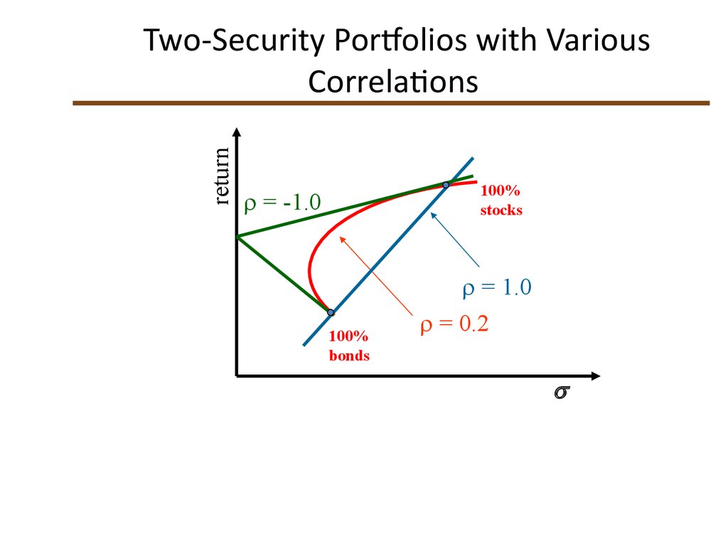
23. Two-Security Portfolios with Various Correlations
returnTwo-Security Portfolios with Various
Correlations
100%
stocks
= -1.0
100%
bonds
= 1.0
= 0.2
24. Portfolio Risk/Return Two Securities: Correlation Effects
• Relationship depends on correlationcoefficient
• -1.0 < < +1.0
• The smaller the correlation, the greater the
risk reduction potential
• If = +1.0, no risk reduction is possible
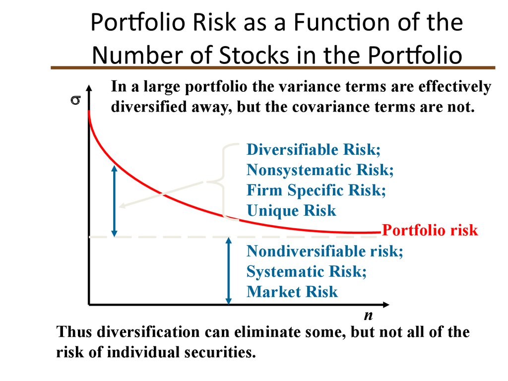
25. Portfolio Risk as a Function of the Number of Stocks in the Portfolio
In a large portfolio the variance terms are effectivelydiversified away, but the covariance terms are not.
Diversifiable Risk;
Nonsystematic Risk;
Firm Specific Risk;
Unique Risk
Portfolio risk
Nondiversifiable risk;
Systematic Risk;
Market Risk
n
Thus diversification can eliminate some, but not all of the
risk of individual securities.
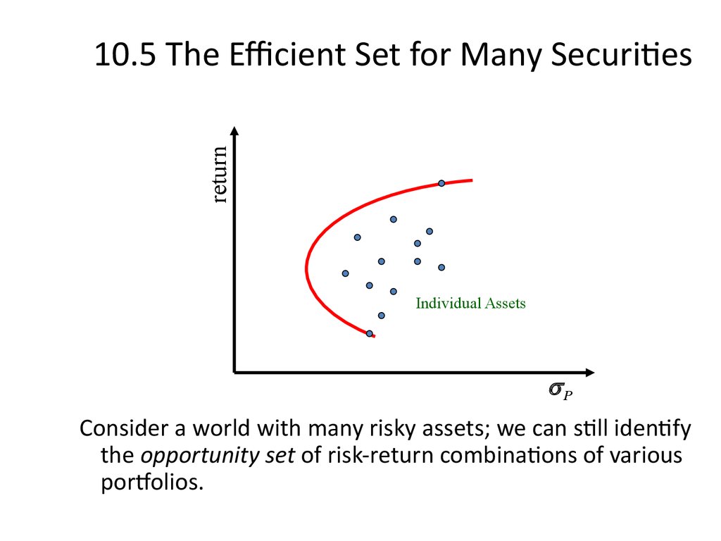
26. 10.5 The Efficient Set for Many Securities
return10.5 The Efficient Set for Many Securities
Individual Assets
P
Consider a world with many risky assets; we can still identify
the opportunity set of risk-return combinations of various
portfolios.
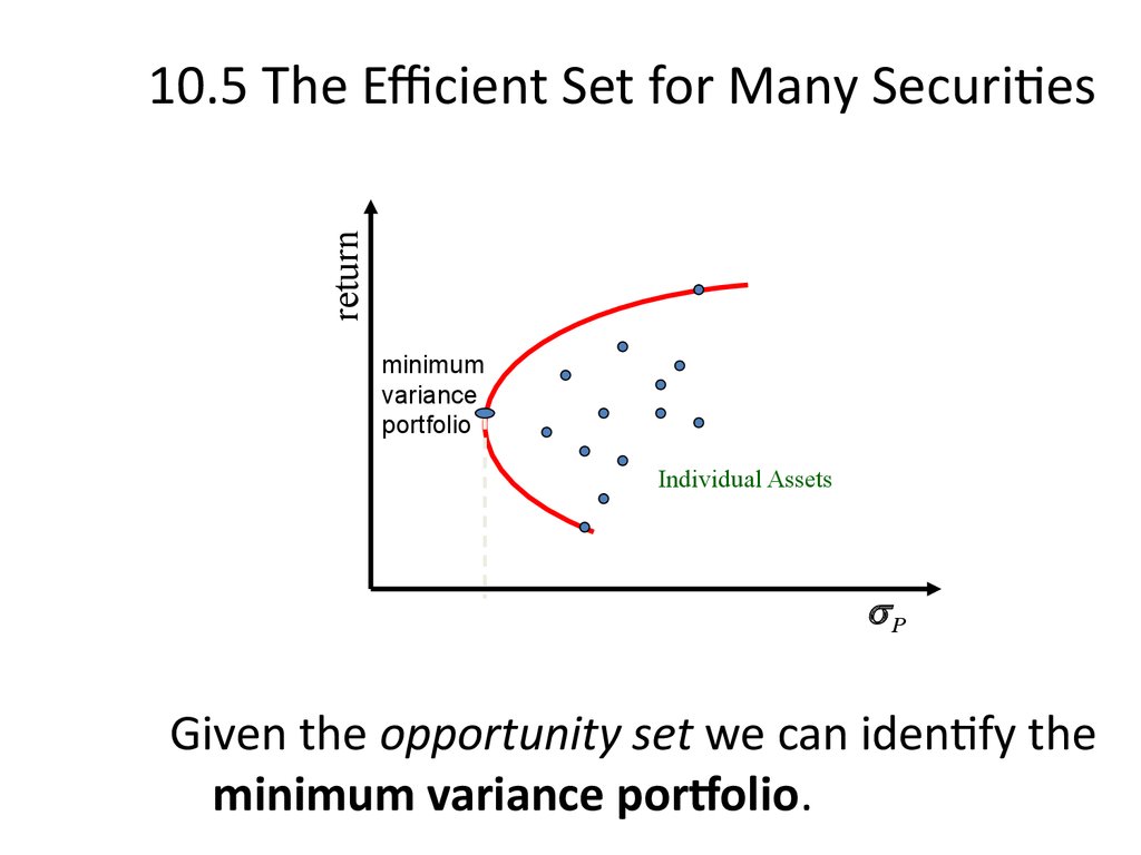
27. 10.5 The Efficient Set for Many Securities
return10.5 The Efficient Set for Many Securities
minimum
variance
portfolio
Individual Assets
P
Given the opportunity set we can identify the
minimum variance portfolio.
28. 10.5 The Efficient Set for Many Securities
return10.5 The Efficient Set for Many Securities
cie
i
f
f
e
tier
n
o
r
nt f
minimum
variance
portfolio
Individual Assets
P
The section of the opportunity set above the
minimum variance portfolio is the efficient frontier.
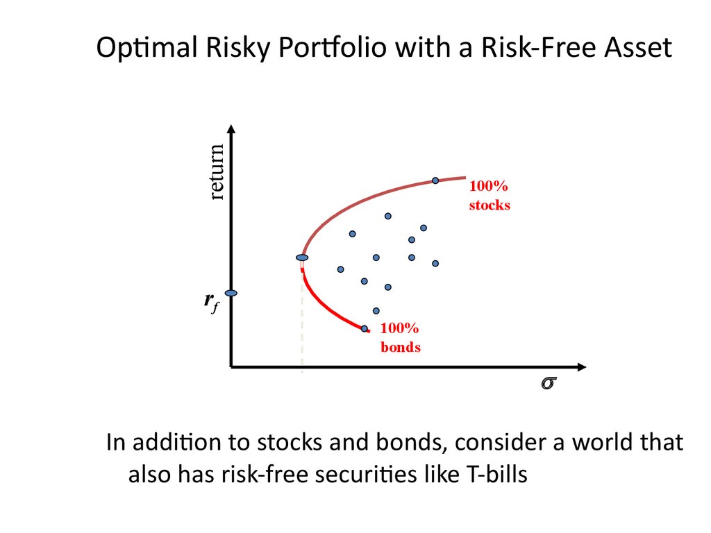
29. Optimal Risky Portfolio with a Risk-Free Asset
returnOptimal Risky Portfolio with a Risk-Free Asset
100%
stocks
rf
100%
bonds
In addition to stocks and bonds, consider a world that
also has risk-free securities like T-bills
30. 10.7 Riskless Borrowing and Lending
return10.7 Riskless Borrowing and Lending
CM
L
100%
stocks
Balanced
fund
rf
100%
bonds
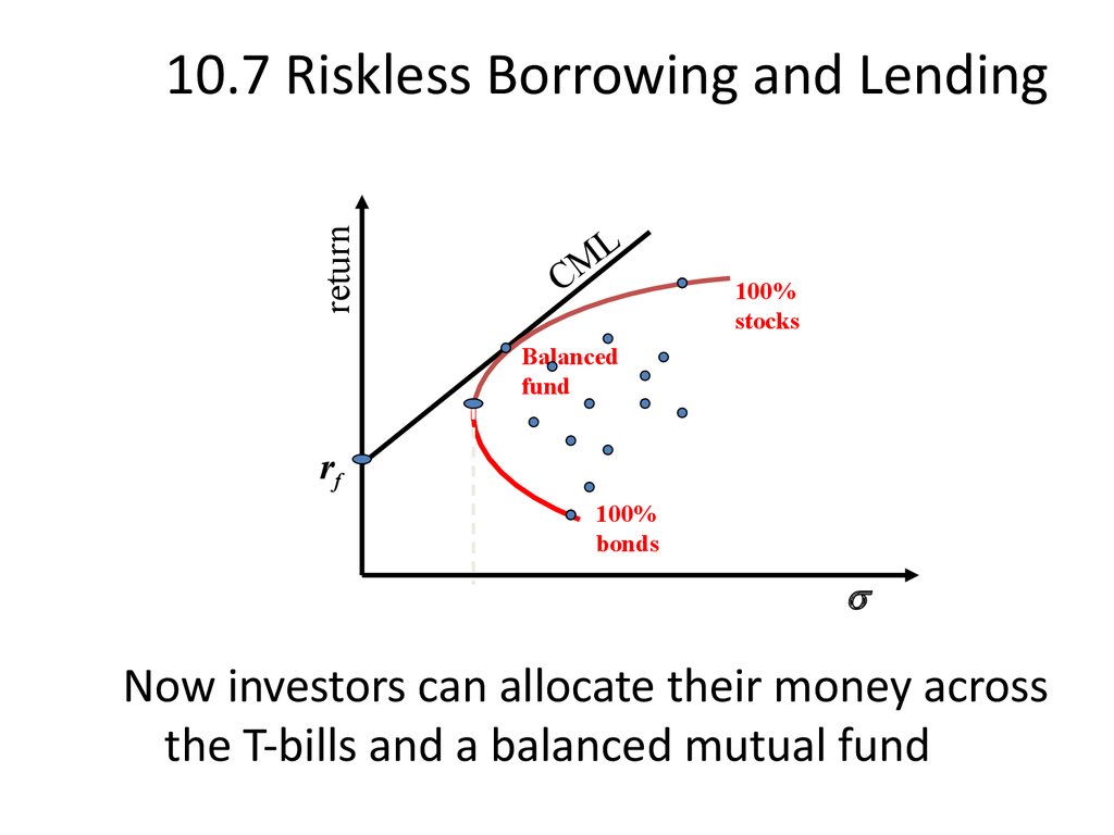
Now investors can allocate their money across
the T-bills and a balanced mutual fund
31. 10.7 Riskless Borrowing and Lending
return10.7 Riskless Borrowing and Lending
L
CM
efficient frontier
rf
P
With a risk-free asset available and the efficient
frontier identified, we choose the capital allocation
line with the steepest slope
32. 10.8 Market Equilibrium
return10.8 Market Equilibrium
CM
L
efficient frontier
M
rf
P
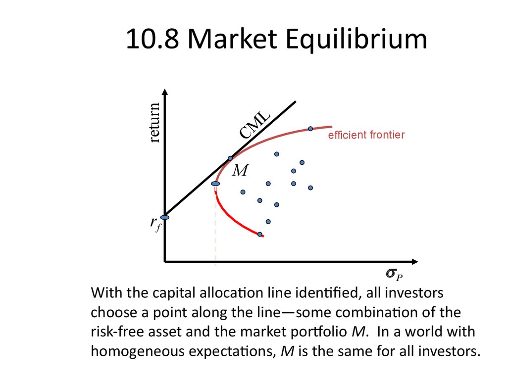
With the capital allocation line identified, all investors
choose a point along the line—some combination of the
risk-free asset and the market portfolio M. In a world with
homogeneous expectations, M is the same for all investors.
33. The Separation Property
returnThe Separation Property
CM
L
efficient frontier
M
rf
P
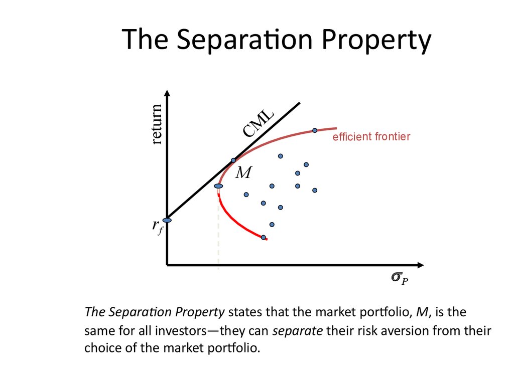
The Separation Property states that the market portfolio, M, is the
same for all investors—they can separate their risk aversion from their
choice of the market portfolio.
34. The Separation Property
returnThe Separation Property
CM
L
efficient frontier
M
rf
P
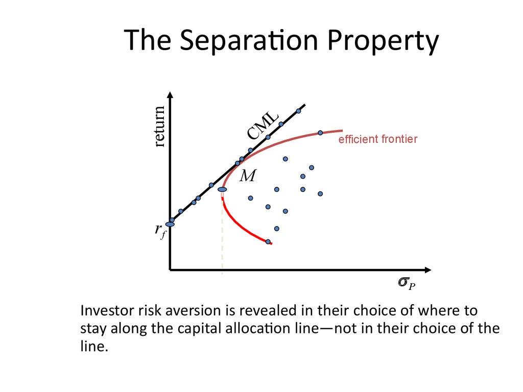
Investor risk aversion is revealed in their choice of where to
stay along the capital allocation line—not in their choice of the
line.
35. Market Equilibrium
returnMarket Equilibrium
CM
L
100%
stocks
Balanced
fund
rf
100%
bonds
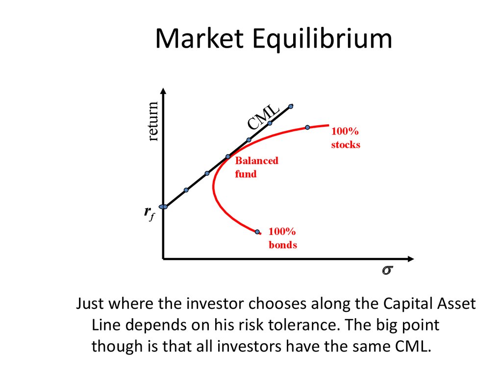
Just where the investor chooses along the Capital Asset
Line depends on his risk tolerance. The big point
though is that all investors have the same CML.
36. Market Equilibrium
returnMarket Equilibrium
CM
L
100%
stocks
Optimal
Risky
Porfolio
rf
100%
bonds
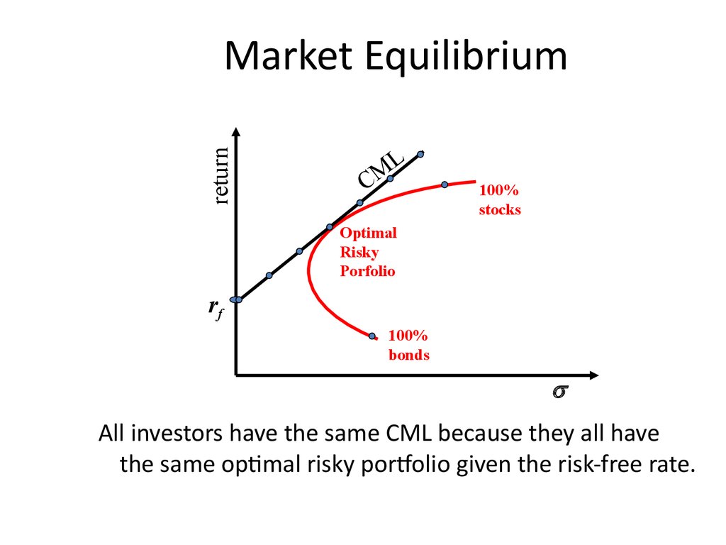
All investors have the same CML because they all have
the same optimal risky portfolio given the risk-free rate.
37. The Separation Property
returnThe Separation Property
CM
L
100%
stocks
Optimal
Risky
Porfolio
rf
100%
bonds
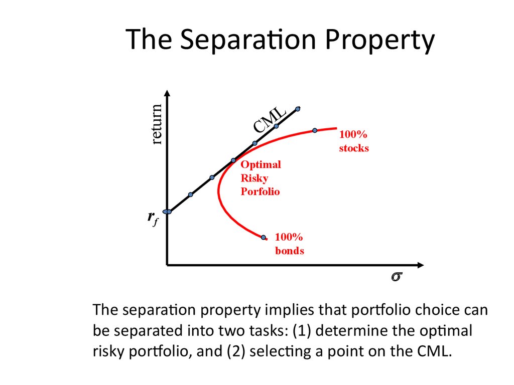
The separation property implies that portfolio choice can
be separated into two tasks: (1) determine the optimal
risky portfolio, and (2) selecting a point on the CML.
38. Optimal Risky Portfolio with a Risk-Free Asset
returnOptimal Risky Portfolio with a Risk-Free Asset
1
f
0
f
r
r
L 0 CML 1
CM
100%
stocks
First
Optimal
Risky
Portfolio
Second Optimal
Risky Portfolio
100%
bonds
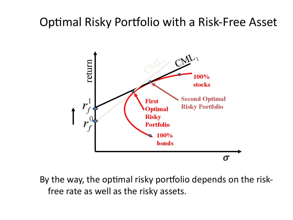
By the way, the optimal risky portfolio depends on the riskfree rate as well as the risky assets.
39. Definition of Risk When Investors Hold the Market Portfolio
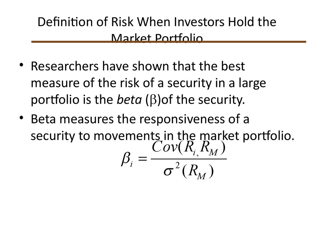
• Researchers have shown that the bestmeasure of the risk of a security in a large
portfolio is the beta (b)of the security.
• Beta measures the responsiveness of a
security to movements in the market portfolio.
bi
Cov( Ri , RM )
( RM )
2
40. Estimating b with regression
Security ReturnsEstimating b with regression
r
e
t
c
a
ar
h
C
c
i
t
is
ne
i
L
Slope = b i
Return on
market %
Ri = a i + b iRm + ei
41. Estimates of b for Selected Stocks
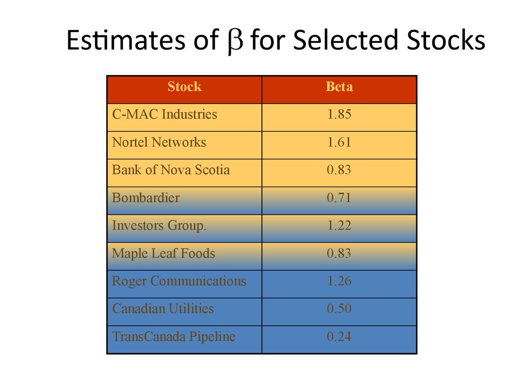
StockBeta
C-MAC Industries
1.85
Nortel Networks
1.61
Bank of Nova Scotia
0.83
Bombardier
0.71
Investors Group.
1.22
Maple Leaf Foods
0.83
Roger Communications
1.26
Canadian Utilities
0.50
TransCanada Pipeline
0.24
42. The Formula for Beta
biCov( Ri , RM )
( RM )
2
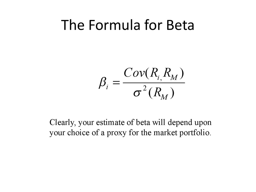
Clearly, your estimate of beta will depend upon
your choice of a proxy for the market portfolio.
43. 10.9 Relationship between Risk and Expected Return (CAPM)
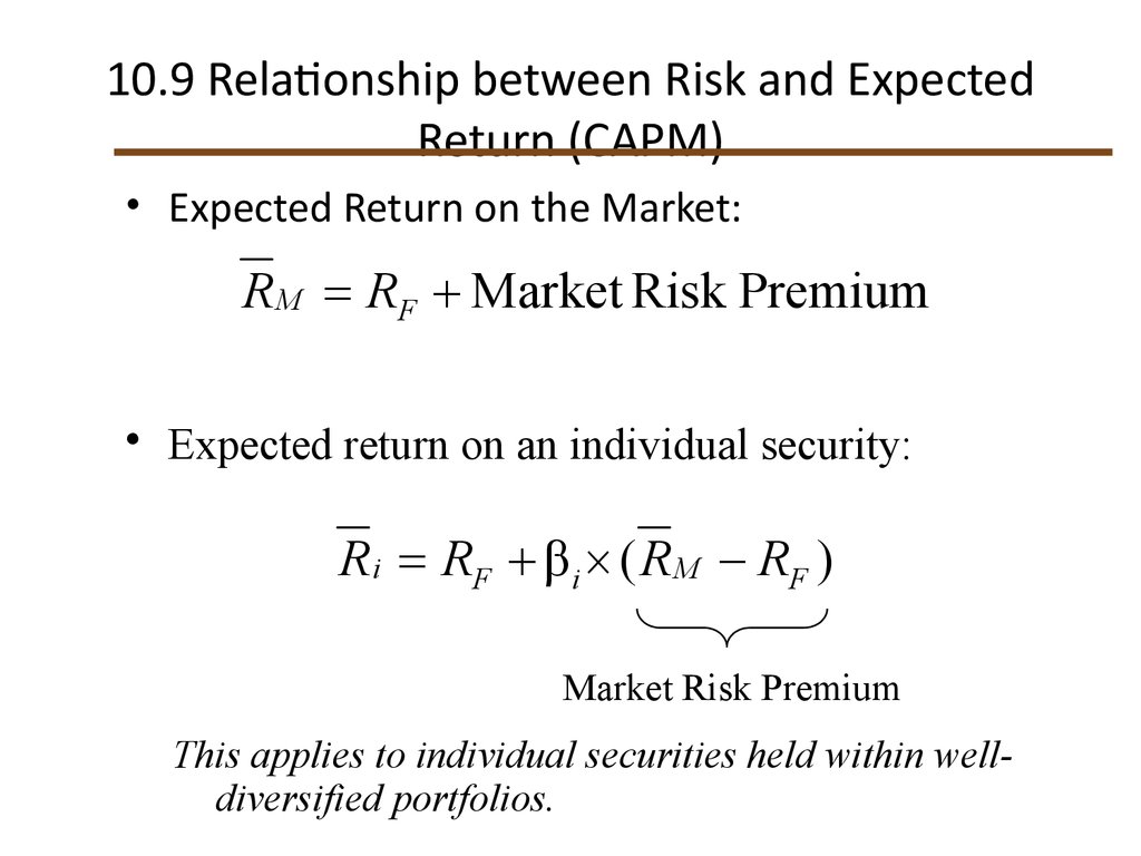
• Expected Return on the Market:R M RF Market Risk Premium
• Expected return on an individual security:
R i RF β i ( R M RF )
Market Risk Premium
This applies to individual securities held within welldiversified portfolios.
44. Expected Return on an Individual Security
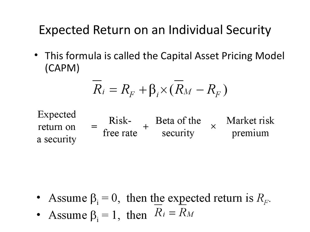
• This formula is called the Capital Asset Pricing Model(CAPM)
R i RF β i ( R M RF )
Expected
return on
a security
RiskBeta of the
=
+
×
free rate
security
Market risk
premium
• Assume bi = 0, then the expected return is RF.
• Assume bi = 1, then R i R M
45. Relationship Between Risk & Expected Return
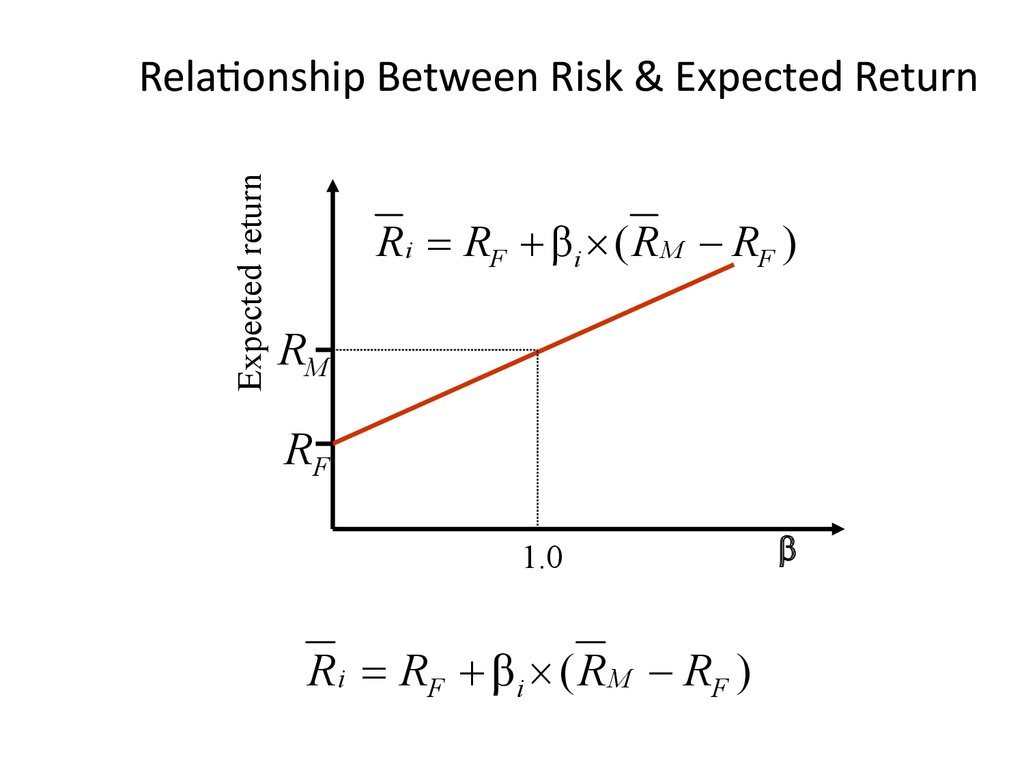
Expected returnRelationship Between Risk & Expected Return
R i RF β i ( R M RF )
RM
RF
1.0
R i RF β i ( R M RF )
b
46. Relationship Between Risk & Expected Return
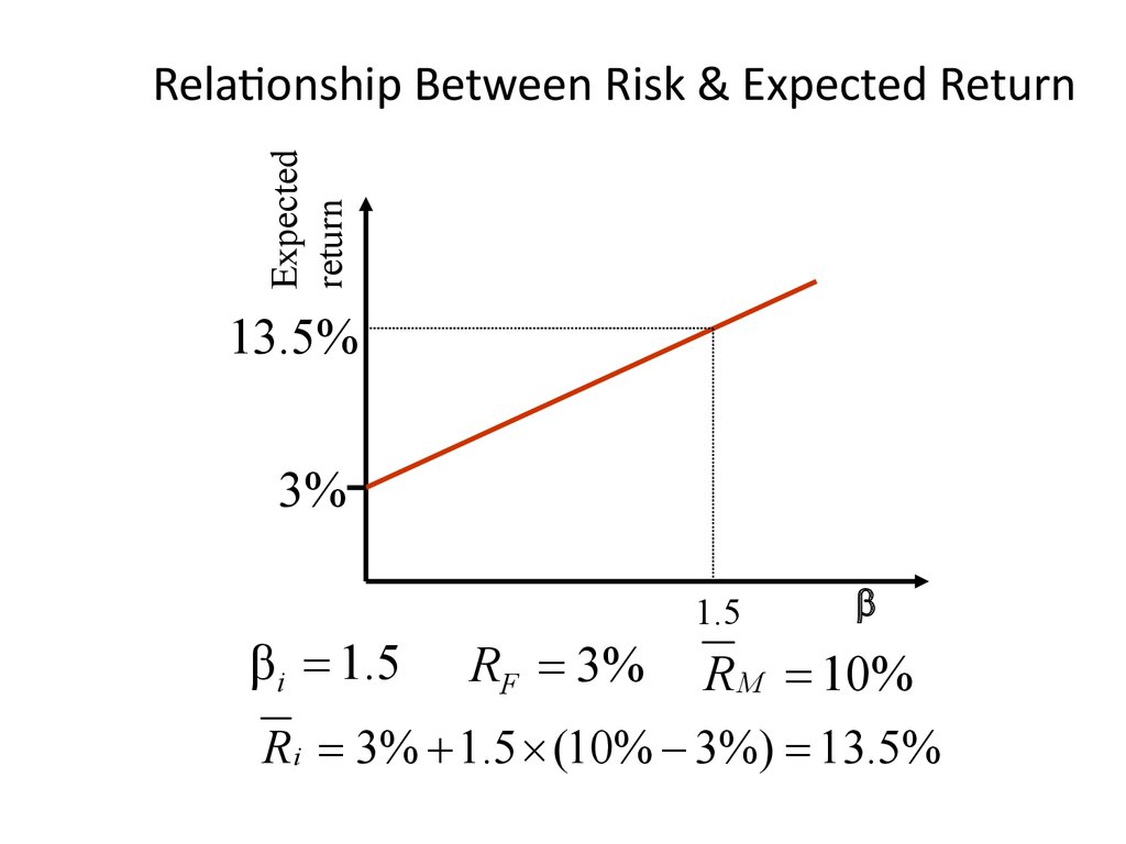
Expectedreturn
Relationship Between Risk & Expected Return
13.5%
3%
β i 1.5
RF 3%
1.5
b
R M 10%
R i 3% 1.5 (10% 3%) 13.5%
47. 10.10 Summary and Conclusions
• This chapter sets forth the principles of modernportfolio theory.
• The expected return and variance on a portfolio of
two securities A and B are given by
E (rP ) wA E (rA ) wB E (rB )
σ P2 (wAσ A )2 (wB σ B )2 2(wB σ B )(wAσ A )ρ AB
• By varying wA, one can trace out the efficient set of
portfolios. We graphed the efficient set for the two-asset case
as a curve, pointing out that the degree of curvature reflects
the diversification effect: the lower the correlation between
the two securities, the greater the diversification.
• The same general shape holds in a world of many assets.
48. 10.10 Summary and Conclusions
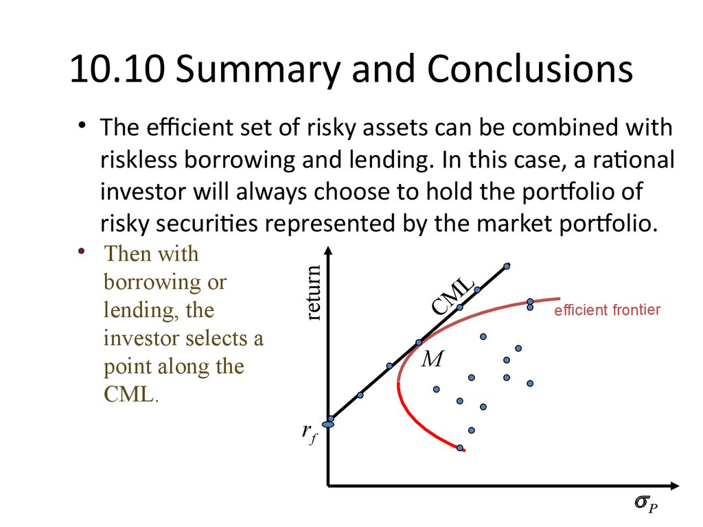
• Then withborrowing or
lending, the
investor selects a
point along the
CML.
return
• The efficient set of risky assets can be combined with
riskless borrowing and lending. In this case, a rational
investor will always choose to hold the portfolio of
risky securities represented by the market portfolio.
CM
L
efficient frontier
M
rf
P
49. 10.10 Summary and Conclusions
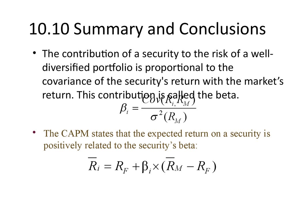
• The contribution of a security to the risk of a welldiversified portfolio is proportional to thecovariance of the security's return with the market’s
return. This contribution
the beta.
Covis( Rcalled
R
)
i, M
bi
2 ( RM )
• The CAPM states that the expected return on a security is
positively related to the security’s beta:
R i RF β i ( R M RF )















 finance


