The definition of a computer system pefmoRmance metrics

1. The definition of a computer system pefmoRmance metrics

THE
DEFINITION
OF
A
COMPUTER
SYSTEM
PEFMORMANCE METRICS

2.

Estimating the performance of computing systems
The basis for comparing different types of computers with each other is given by standard methods of
measuring productivity [26, 54]. In the development of computer technology, several such standard
techniques have emerged. They allow developers and users to choose between alternatives based on
quantitative indicators, which allows for continuous progress in this area.
The unit of measurement of computer performance is time: a computer that performs the same amount
of work in less time is faster. The execution time of any program is measured in seconds. Often,
performance is measured as the rate of occurrence of a certain number of events per second, so a
shorter time implies greater performance.
However, depending on what we believe, time can be determined in various ways. The simplest way to
determine time is called astronomical time, response time, execution time, or elapsed time. This is a
delay in the task, which includes literally everything: processor operation, disk accesses, memory
accesses, I / O and operating system overhead. However, when working in multiprogram mode while
waiting for I / O for one program, the processor can execute another program, and the system will not
necessarily minimize the execution time of this particular program.
To measure the processor's operating time, a special parameter is used in this program - CPU time,
which does not include the I / O timeout or the execution time of another program. Obviously, the
response time seen by the user is the total execution time of the program, not the CPU time. The CPU
time can be further divided by the time spent by the CPU directly on the execution of the user program
and called the CPU user time, and the CPU time spent by the operating system on the execution of the
tasks requested by the program, and called CPU time.

3.

In some cases, the system time of the CPU is ignored because of the possible inaccuracy of the
measurements performed by the operating system itself, and also because of the problems associated
with comparing the performance of machines with different operating systems. On the other hand, the
system code on some machines is the user code on others and, in addition, almost no program can
work without some operating system. Therefore, when measuring the processor's performance, the
amount of user and system CPU time is often used.
In most modern processors, the speed of the processes of interaction of internal functional devices is
determined not by natural delays in these devices, but is determined by a single system of clock signals
generated by some clock generator, usually operating at a constant speed. Discrete time events are
called clock cycles, ticks, clock periods, cycles, or clock cycles. Computer designers usually talk about
a synchronization period, which is determined either by its duration (for example, 10 nanoseconds) or
by the frequency (for example, 100 MHz). The length of the synchronization period is the inverse of the
synchronization frequency.

4.

Thus, the CPU time for some program can be expressed in two ways: the number of clock cycles for a
given program, multiplied by the duration of the synchronization clock, or the number of clock cycles for
a given program divided by the synchronization frequency.
An important characteristic, often published in the reports on processors, is the average number of
clock cycles per command - CPI (clock cycles per instruction). With a certain number of executable
commands in the program, this parameter allows you to quickly estimate the CPU time for this program.
Thus, the CPU performance depends on three parameters: the clock cycle (or frequency), the average
number of cycles per command, and the number of commands executed. It is impossible to change any
of these parameters isolated from the other, because the underlying technologies used to change each
of these parameters are interrelated: the synchronization frequency is determined by the hardware
technology and the functional organization of the processor; the average number of cycles per
command depends on the functional organization and architecture of the command system; and the
number of commands executed in the program is determined by the architecture of the command
system and compiler technology. When comparing two machines, you need to consider all three
components to understand relative performance.

5.

In the process of searching, what would you not know, whatever it was. In fact, the only suitable and
reliable unit for measuring time is the running time of real programs, and all proposed replacements of
this time in accordance with standard programs are only misleading.
The dangers of some popular alternative measurements (MIPS and MFLOPS) will be discussed in the
corresponding sections of the chapters.

6.

MIPS
One of the alternative units for measuring the processor's performance (relative to the execution time)
is MIPS - (one million instructions per second). There are several different options for interpreting the
definition of MIPS.
In general, MIPS is the rate of operations per unit of time, i.e. for any given MIPS program there is
simply the ratio of the number of instructions in the program to the time of its execution. Thus,
performance can be defined as a reverse-to-time value, and faster machines will have a higher MIPS
rating.

7.

The positive aspects of MIPS is that this characteristic is easy to understand, especially to the buyer,
and that a faster machine is characterized by a large number of MIPS, which corresponds to our
intuitive notions. However, using MIPS as a metric for comparison encounters three problems. First,
MIPS depends on a set of processor instructions, which makes it difficult to compare MIPS computers
that have different command systems. Secondly, MIPS even on the same computer varies from
program to program. Thirdly, MIPS can change in relation to performance in the opposite direction.
A classic example for the latter case is the MIPS rating for a machine that includes a floating-point
coprocessor. Since in general, more synchronization cycles are required for each floating point
command than for an integer command, programs using the floating point coprocessor instead of the
corresponding subroutines from the software are executed in less time, but have a lower MIPS rating.
In the absence of a coprocessor, floating-point operations are performed using subroutines that use
simpler integer arithmetic commands, and as a consequence, such machines have a higher MIPS
rating, but perform so many commands that the total execution time is significantly increased. Similar
anomalies are observed when using optimizing compilers, when optimization results in a reduction in
the number of commands executed in the program, the MIPS rating is reduced and productivity is
increased.
Another definition of MIPS is associated with the very popular once computer VAX 11/780 company
DEC. It was this computer that was adopted as a benchmark for comparing the performance of various
machines. It was believed that the performance of the VAX 11/780 is 1 MIPS (one million instructions
per second).

8.

At that time, the synthetic test Dhrystone was widespread, which allowed to evaluate the efficiency of
processors and compilers from the C language for non-numeric processing programs. It was a test mix,
53% of which were assignment operators, 32% - control operators and 15% - function calls. It was a
very short test: the total number of teams was 100. The speed of execution of the program from these
100 teams was measured in Dhrystone per second. The performance of the VAX 11/780 on this
synthetic test was 1757 Dhrystone per second. Thus, 1 MIPS is equal to 1757 Dhrystone per second.
It should be noted that at present the Dhrystone test is practically not applied. The small volume allows
you to place all test commands in the cache of the first level of a modern microprocessor, and it does
not even allow you to assess the effect of having a second level cache, although it can well reflect the
effect of increasing the clock frequency.
The third definition of MIPS is related to the IBM RS / 6000 MIPS. The fact is that a number of
manufacturers and users (followers of IBM) prefer to compare the performance of their computers with
the performance of modern IBM computers, and not with the old DEC machine. The relationship
between VAX MIPS and RS / 6000 MIPS was never widely published, but 1 RS / 6000 MIPS is
approximately equal to 1.6 VAX 11/780 MIPS.

9.

MFLOPS
Measuring the performance of computers in solving scientific and technical problems, in
which floating-point arithmetic is used, has always been of particular interest. It was for
such calculations that the first question arose about measuring performance, and on the
achieved indicators, conclusions were often drawn about the overall level of computer
development. Usually for scientific and technical tasks, the processor's performance is
estimated in MFLOPS (millions of floating-point results per second, or millions of
elementary arithmetic operations on floating-point numbers performed per second).

10.

As a unit of measure, MFLOPS is designed to evaluate the performance of only floating point
operations and therefore is not applicable outside this limited area. For example, compiler programs
have a MFLOPS rating close to zero, no matter how fast the machine is, since compilers rarely use
floating-point arithmetic.
It is clear that the MFLOPS rating depends on the machine and the program. This term is less harmless
than MIPS. It is based on the number of operations performed, and not on the number of commands
executed. According to many programmers, the same program running on different computers will
perform a different number of instructions, but the same number of operations with a floating point. That
is why the MFLOPS rating was intended for a fair comparison of different machines among themselves.
However, with MFLOPS everything is not so cloudless. First of all, this is due to the fact that sets of
floating point operations are not compatible on different computers. For example, in the
supercomputers of Cray Research [1] there is no division command (there is, of course, an operation
for calculating the reciprocal of a floating-point number, and the division operation can be implemented
by multiplying a divisor divisible by a reciprocal of the divisor). At the same time, many modern
microprocessors have division commands, calculating the square root, sine and cosine.
Another, realized by all, problem lies in the fact that the MFLOPS rating changes not only on a mixture
of integer operations and floating-point operations, but also on a mixture of fast and slow floating-point
operations. For example, a program with 100% addition operations will have a higher rating than a
program with 100% division operations.

11.

The solution to both problems is to take the "canonical" or "normalized" number of floating point
operations from the source code of the program and then divide it into runtime. Table 1 shows how the
authors of the "Livermore Cycles" test package, which will be discussed below, calculate the number of
normalized floating-point operations for the program in accordance with the operations actually located
in its source text. Thus, the actual MFLOPS rating is different from the normalized MFLOPS rating,
which is often cited in the supercomputer literature.
Most often, MFLOPS, as a unit of performance measurement, is used in carrying out control tests on
the test packages "Livermore Cycles" and LINPACK
Livermore cycles are a set of fragments of fortran programs, each of which is taken from real software
systems operated by the Livermore National Laboratory. Lawrence [2] (USA). Usually, during the tests,
either a small set of 14 cycles or a large set of 24 cycles is used.
The Livermore cycle is used to evaluate the performance of computers since the mid-1960s. Livermore
cycles are considered typical fragments of programs of numerical problems. The emergence of new
types of machines, including vector and parallel, did not diminish the importance of the Livermore
cycles, but the values of productivity and the magnitude of the variation between different cycles
changed.
On a vector machine, the performance depends not only on the element base, but also on the nature of
the algorithm itself, i.e. coefficient of vectorizability. Among the Livermore cycles, the coefficient of
vectorizability ranges from 0 to 100%, which once again confirms their value for evaluating the
performance of vector architectures. In addition to the nature of the algorithm, the vectorization factor is
also affected by the quality of the vectorizer built into the compiler.

12.

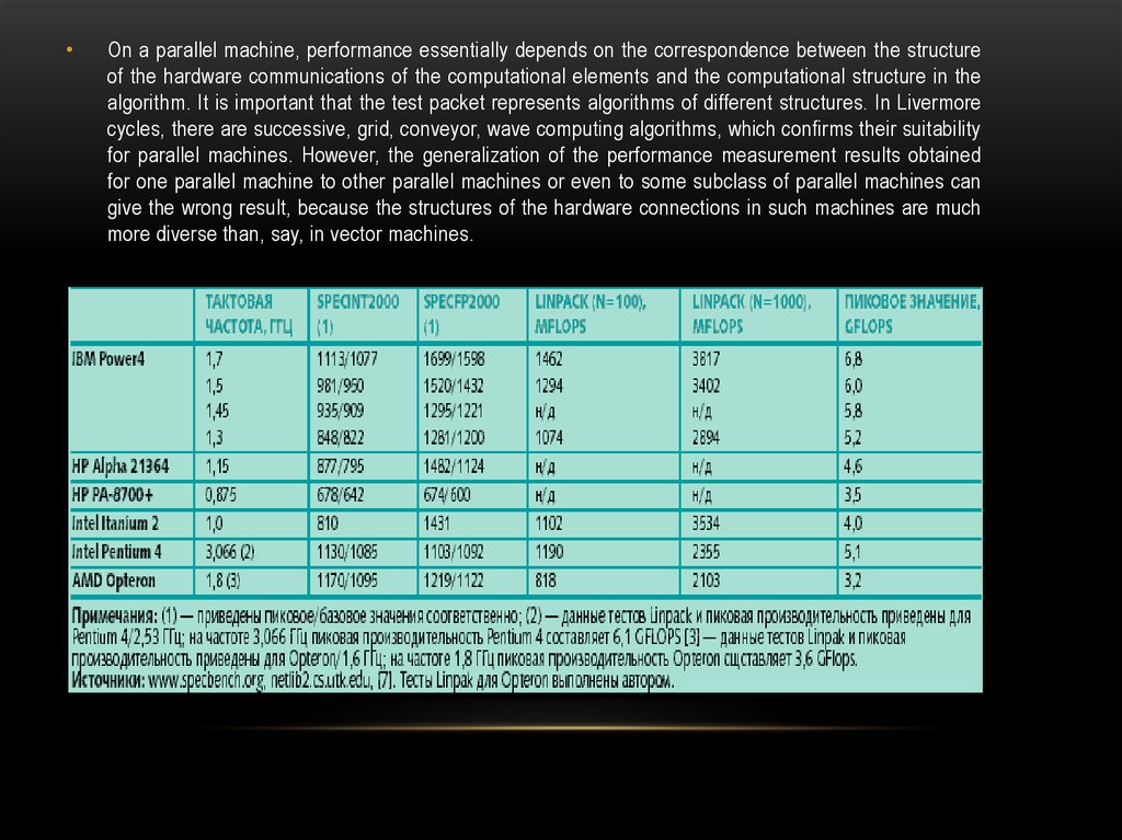
On a parallel machine, performance essentially depends on the correspondence between the structure
of the hardware communications of the computational elements and the computational structure in the
algorithm. It is important that the test packet represents algorithms of different structures. In Livermore
cycles, there are successive, grid, conveyor, wave computing algorithms, which confirms their suitability
for parallel machines. However, the generalization of the performance measurement results obtained
for one parallel machine to other parallel machines or even to some subclass of parallel machines can
give the wrong result, because the structures of the hardware connections in such machines are much
more diverse than, say, in vector machines.

13.

LINPACK is a package of fortran programs for solving systems of linear algebraic equations. The goal
of creating LINPACK was not to measure performance. Algorithms of linear algebra are very widely
used in a variety of tasks, and therefore measuring performance on LINPACK is of interest to many
users. Information about the performance of various machines on the LINPACK package is published
by the employee of the Argonne National Laboratory (USA) J. Dongarroi [3] [65] and is periodically
updated

14.

The algorithms of the current version of LINPACK are based on the decomposition method. The initial
matrix of 100x100 elements (in the last version of 1000x1000) is first represented as a product of two
matrices of the standard structure, over which the algorithm for finding the solution is then executed.
Subroutines included in LINPACK are structured. In the standard version of LINPACK, the internal level
of the basic routines is highlighted, each of which performs an elementary operation on vectors. A set of
basic routines is called BLAS (Basic Linear Algebra Subprograms). For example, BLAS includes two
simple SAXPY subprograms (vector multiplication by scalar and vector addition) and SDOT (scalar
product of vectors). All operations are performed on floating-point numbers represented with double
precision. The result is measured in MFLOPS.
Using the results of the LINPACK double-precision test package as a basis for demonstrating the
MFLOPS rating has become a common practice in the computer industry. It should be remembered that
when using the original matrix of 100x100, it can be completely placed in a cache memory of capacity,
for example, 1 MB. If a 1000x1000 matrix is used during the tests, then the capacity of such a cache is
already insufficient and some memory accesses will be accelerated due to the presence of such a
cache, while others will lead to slips and require more time to process memory accesses. For
multiprocessor systems there are also parallel versions of LINPACK, and such systems often show a
linear increase in performance with an increase in the number of processors.

15.

However, like any other unit of measurement, the MFLOPS rating for a single program can not be
generalized for all occasions to represent a single unit of computer performance, although it is tempting
to characterize the machine with a single MIPS or MFLOPS rating without specifying a program.