3.56M

Multimedia computing Geometric Processesing__lec16

1.

Multimedia Computing
By
Minhaz Uddin Ahmed, PhD
Department of Computer Engineering
Inha University in Tashkent.
Email: [email protected]

2.

Content
Interpolation
Nearest Neighbor interpolation
Bilinear interpolation
Cubic convolution interpolation
Spline interpolation
Image scaling
Minification
Rotation
Translation
Mirroring

3.

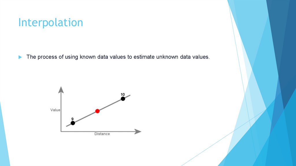
Interpolation
The process of using known data values to estimate unknown data values.

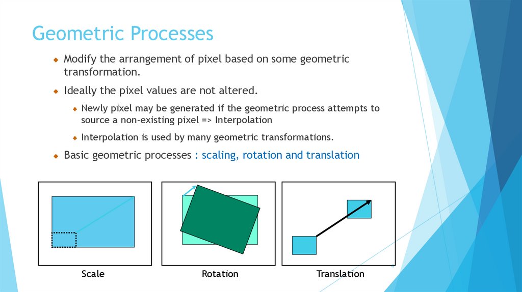
Geometric Processes
Modify the arrangement of pixel based on some geometric
transformation.
Ideally the pixel values are not altered.
Newly pixel may be generated if the geometric process attempts to
source a non-existing pixel => Interpolation
Interpolation is used by many geometric transformations.
Basic geometric processes : scaling, rotation and translation
Scale
Rotation
Translation
4

5.

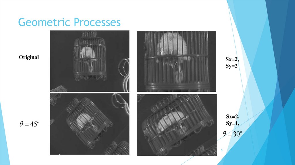
Geometric Processes
Original
Sx=2,
Sy=2
Sx=2,
Sy=1,
45o
30 o
5

6.

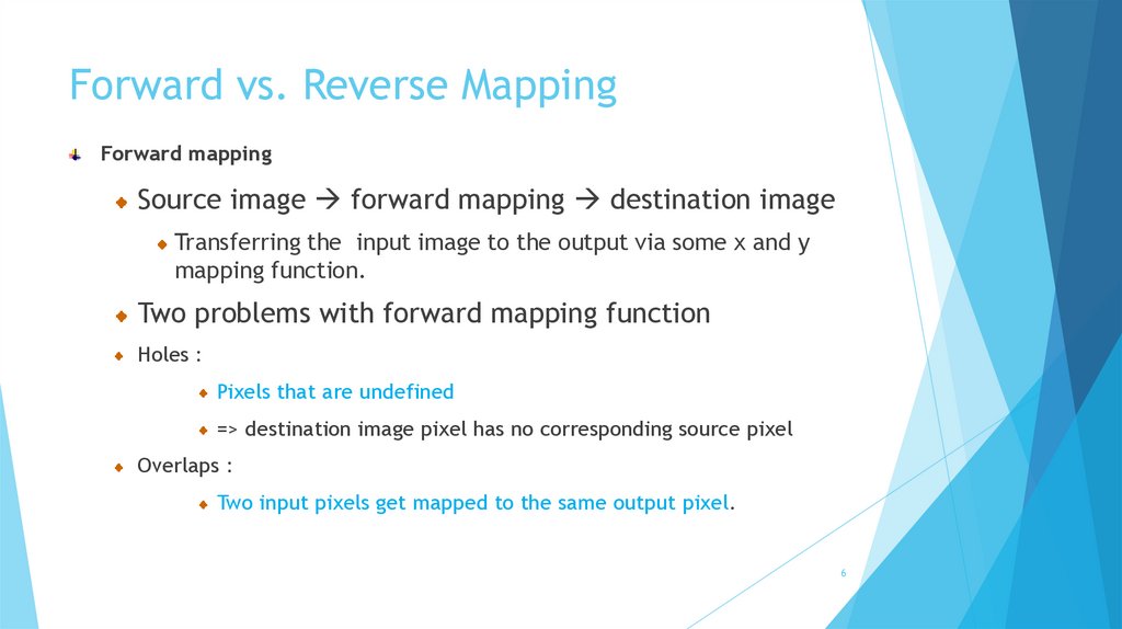
Forward vs. Reverse Mapping
Forward mapping
Source image forward mapping destination image
Transferring the input image to the output via some x and y
mapping function.
Two problems with forward mapping function
Holes :
Pixels that are undefined
=> destination image pixel has no corresponding source pixel
Overlaps :
Two input pixels get mapped to the same output pixel.
6

7.

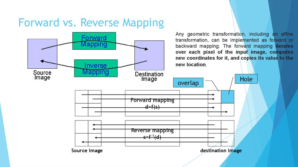
Forward vs. Reverse Mapping
Any geometric transformation, including an affine
transformation, can be implemented as forward or
backward mapping. The forward mapping iterates
over each pixel of the input image, computes
new coordinates for it, and copies its value to the
new location.
overlap
Hole
Forward mapping
d=f(s)
Reverse mapping
s=f-1(d)
Source image
destination
7 image

8.

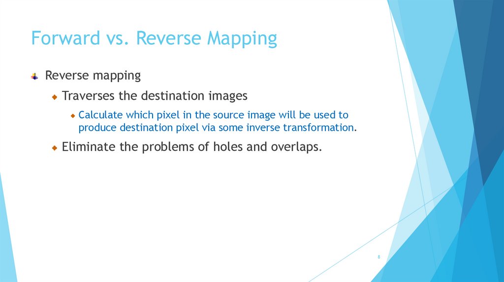
Forward vs. Reverse Mapping
Reverse mapping
Traverses the destination images
Calculate which pixel in the source image will be used to
produce destination pixel via some inverse transformation.
Eliminate the problems of holes and overlaps.
8

9.

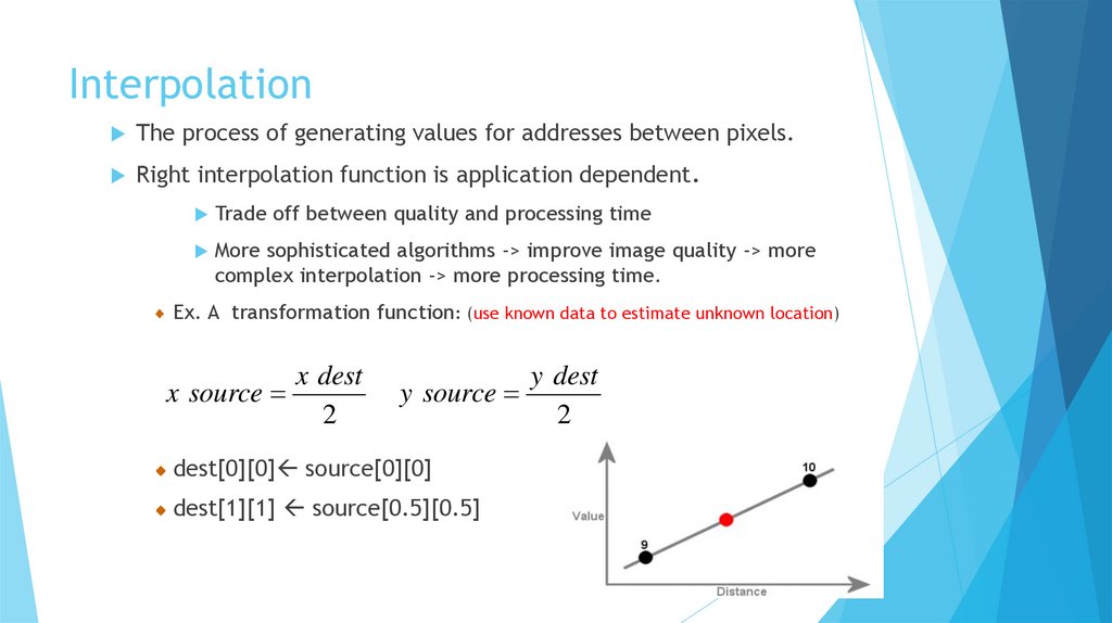
Interpolation
The process of generating values for addresses between pixels.
Right interpolation function is application dependent.
Trade off between quality and processing time
More sophisticated algorithms -> improve image quality -> more
complex interpolation -> more processing time.
Ex. A transformation function: (use known data to estimate unknown location)
x source
x dest
2
y source
dest[0][0] source[0][0]
dest[1][1] source[0.5][0.5]
y dest
2

10.

Interpolation
Interpolation used for zooming , shrinking, rotating and geometric processing.
Zooming requires two steps
The creation of new pixel locations
The assignment of gray levels to these new locations
Techniques for zooming
Nearest Neighbor Interpolation
Bilinear interpolation
Bicubic interpolation

11.

1. Nearest Neighbor Interpolation
Nearest Neighbor Interpolation
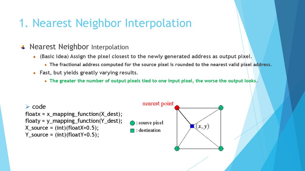
(Basic idea) Assign the pixel closest to the newly generated address as output pixel.
The fractional address computed for the source pixel is rounded to the nearest valid pixel address.
Fast, but yields greatly varying results.
The greater the number of output pixels tied to one input pixel, the worse the output looks.
code
floatx = x_mapping_function(X_dest);
floaty = y_mapping_function(Y_dest);
X_source = (int)(floatX+0.5);
Y_source = (int)(floatY+0.5);
11

12.

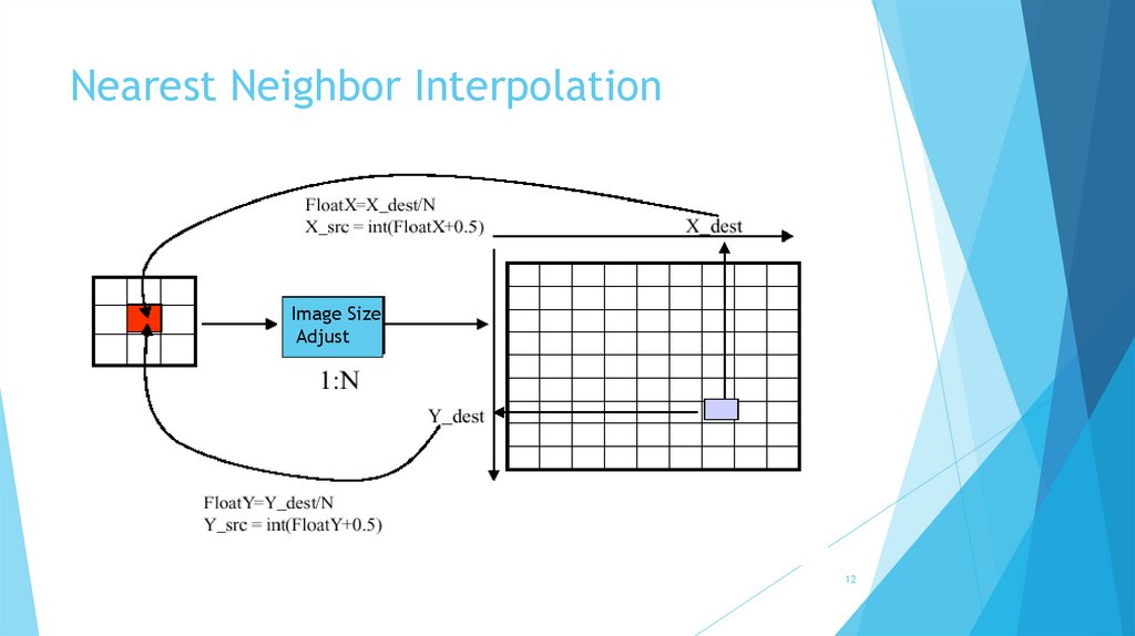
Nearest Neighbor Interpolation
Image Size
Adjust
12

13.

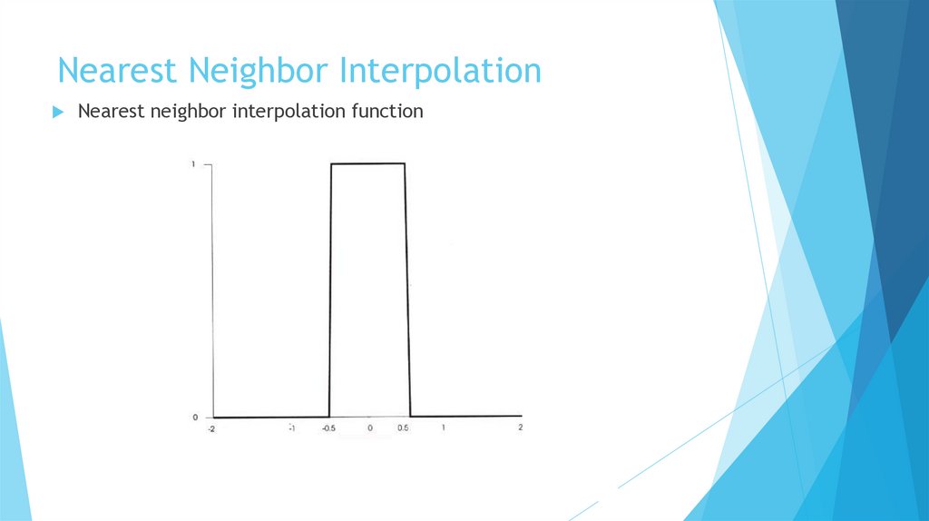
Nearest Neighbor Interpolation
Nearest neighbor interpolation function

14.

Nearest Neighbor Interpolation
Process:
For each non-integer coordinate, find the nearest neighboring pixel.
Assign the value of that nearest pixel to the new location.
Pros:
Simple and computationally inexpensive.
Cons:
The resulting image can appear pixelated, especially when upsampling.

15.

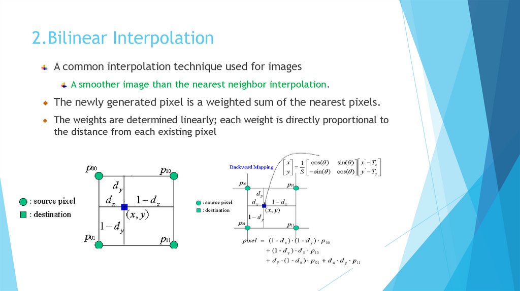
2.Bilinear Interpolation
A common interpolation technique used for images
A smoother image than the nearest neighbor interpolation.
The newly generated pixel is a weighted sum of the nearest pixels.
The weights are determined linearly; each weight is directly proportional to
the distance from each existing pixel

16.

Bilinear Interpolation
Bilinear interpolation considers the closest 2x2 neighborhood of known pixels
surrounding the unknown pixel. The value of the unknown pixel is a weighted
average of these 4 pixels, based on their distance.
Process:
Calculate the horizontal interpolation between two pixels (left and right).
Then, interpolate vertically between the two resulting values.
Pros:
Produces smoother results compared to nearest
neighbor.
Cons:
More computationally expensive than nearest
neighbor.

17.

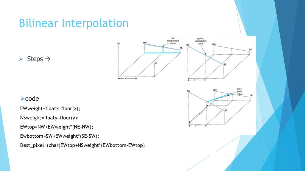
Bilinear Interpolation
Steps
code
EWweight=floatx–floor(x);
NSweight=floaty–floor(y);
EWtop=NW+EWweight*(NE-NW);
Ewbottom=SW+EWweight*(SE-SW);
Dest_pixel=(char)EWtop+NSweight*(EWbottom-EWtop)
17

18.

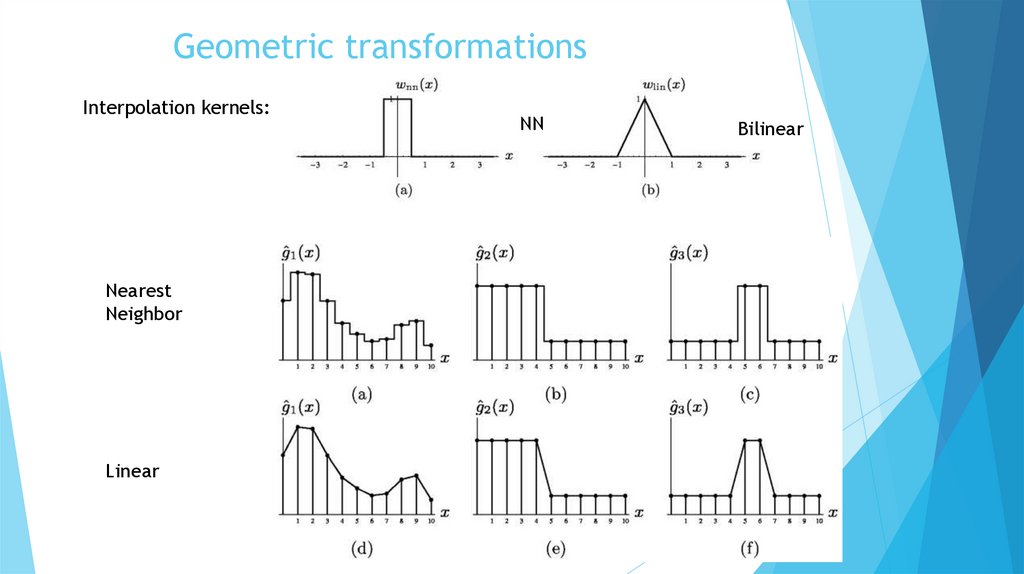
Geometric transformations
Interpolation kernels:
Nearest
Neighbor
Linear
NN
Bilinear

19.

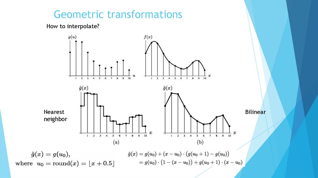
Geometric transformations
How to interpolate?
Nearest
neighbor
Bilinear

20.

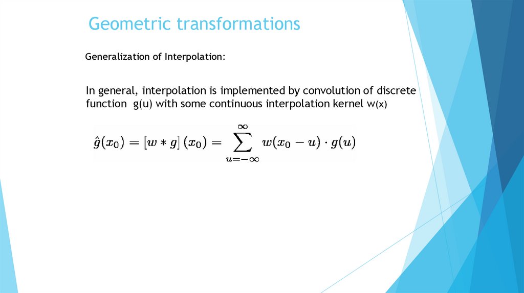
Geometric transformations
Generalization of Interpolation:
In general, interpolation is implemented by convolution of discrete
function g(u) with some continuous interpolation kernel w(x)

21.

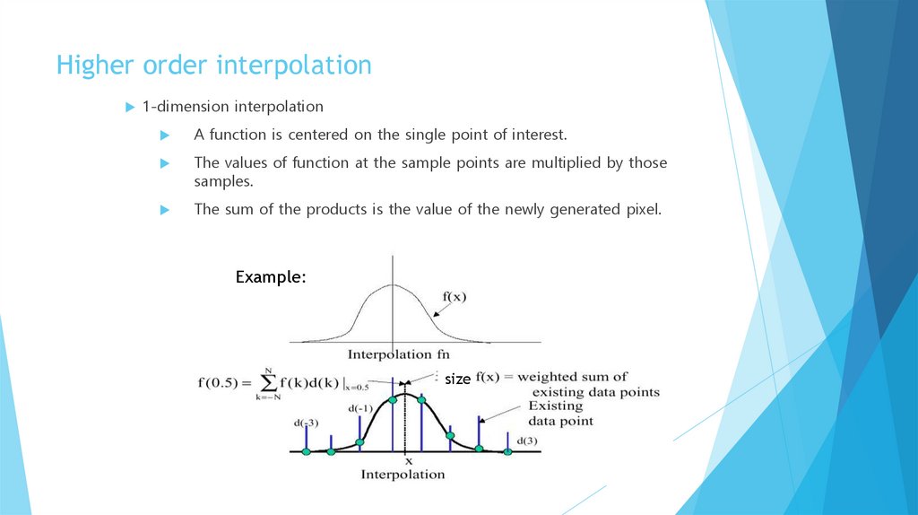
Higher order interpolation
1-dimension interpolation
A function is centered on the single point of interest.
The values of function at the sample points are multiplied by those
samples.
The sum of the products is the value of the newly generated pixel.
Example:
size

22.

Higher order interpolation
Higher order interpolation
Cubic convolution and B-Spline interpolation functions
Requires large areas to generate a new pixel => 16 nearest pixels each
Cf. Nearest neighbor requires 1 pixel, and Bilinear 4 pixels.
Principle of interpolation function processes
A function is centered on the single point of interest.
The values of function at the sample points are multiplied by those
samples.
Sample points: f(-d), f(-1-d), f(1-d), f(2-d), where x is offset from
the nearest left sample by d.
The sum of the products is the value of the newly generated pixel.

23.

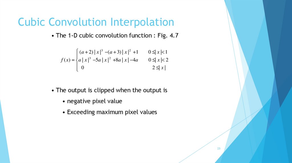
Cubic Convolution Interpolation
• The 1-D cubic convolution function : Fig. 4.7
(a 2) | x | 3 (a 3) | x | 2 1
f ( x) a | x | 3 5a | x | 2 8a | x | 4a
0
0 | x | 1
0 | x | 2
2 | x |
• The output is clipped when the output is
• negative pixel value
• Exceeding maximum pixel values
23

24.

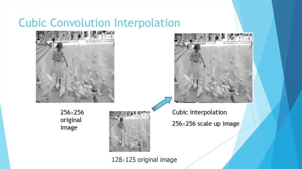
Cubic Convolution Interpolation
256 256
original
image
Cubic interpolation
256 256 scale up image
128 125 original image

25.

3. Bicubic Interpolation
Bicubic interpolation goes one step further than bilinear interpolation by
considering the closest 4x4 neighborhood of known pixels. It calculates the
weighted average of these 16 pixels, offering even smoother results.
Process:
Use cubic polynomials to interpolate along the x-axis and y-axis, using a 4x4 grid of
surrounding pixels.

26.

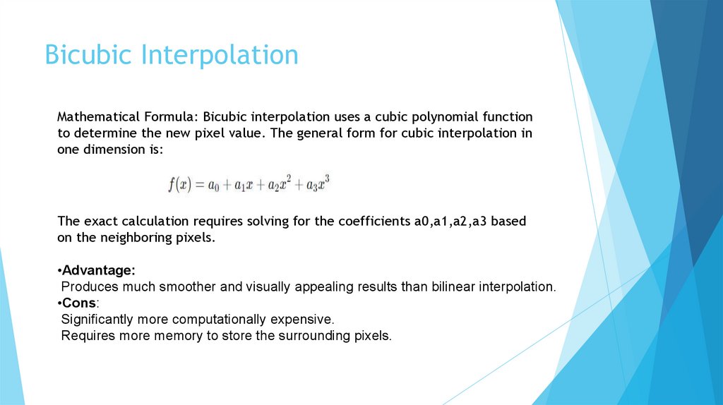
Bicubic Interpolation
Mathematical Formula: Bicubic interpolation uses a cubic polynomial function
to determine the new pixel value. The general form for cubic interpolation in
one dimension is:
The exact calculation requires solving for the coefficients a0,a1,a2,a3 based
on the neighboring pixels.
•Advantage:
Produces much smoother and visually appealing results than bilinear interpolation.
•Cons:
Significantly more computationally expensive.
Requires more memory to store the surrounding pixels.

27.

4. Spline Interpolation
Spline interpolation fits a piecewise polynomial to the data points, usually
using cubic splines. It is commonly used for more precise image
transformations and can provide smoother results than bicubic interpolation,
especially in cases where very high-quality results are needed.
Process:
Pros:
Fit a cubic spline (a smooth, continuous curve) to the data points and interpolate
values using that curve.
Can provide smoother results with less visible artifacts.
Cons:
Computationally intensive and more complex to implement.

28.

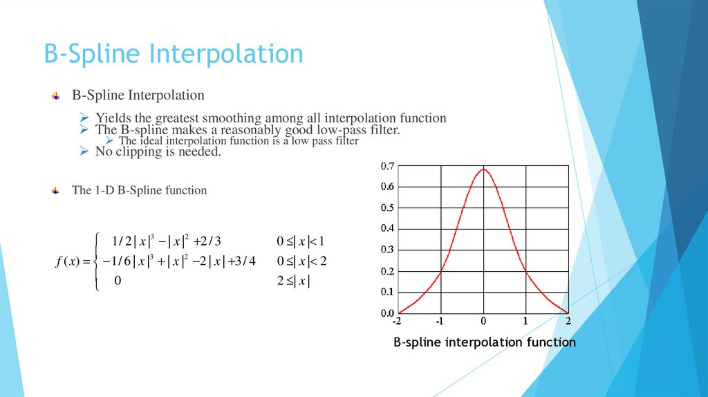
B-Spline Interpolation
B-Spline Interpolation
Yields the greatest smoothing among all interpolation function
The B-spline makes a reasonably good low-pass filter.
The ideal interpolation function is a low pass filter
No clipping is needed.
The 1-D B-Spline function
1 / 2 | x |3 | x |2 2 / 3
f ( x) 1 / 6 | x |3 | x |2 2 | x | 3 / 4
0
0 | x | 1
0 | x | 2
2 | x |
B-spline interpolation function

29.

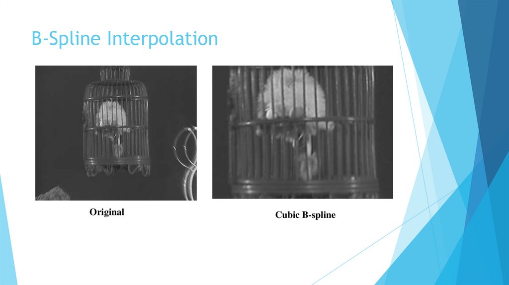
B-Spline Interpolation
Original
Cubic B-spline

30.

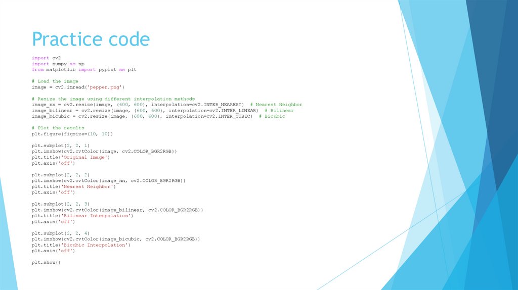
Practice code
import cv2
import numpy as np
from matplotlib import pyplot as plt
# Load the image
image = cv2.imread('pepper.png')
# Resize the image using different interpolation methods
image_nn = cv2.resize(image, (600, 600), interpolation=cv2.INTER_NEAREST) # Nearest Neighbor
image_bilinear = cv2.resize(image, (600, 600), interpolation=cv2.INTER_LINEAR) # Bilinear
image_bicubic = cv2.resize(image, (600, 600), interpolation=cv2.INTER_CUBIC) # Bicubic
# Plot the results
plt.figure(figsize=(10, 10))
plt.subplot(2, 2, 1)
plt.imshow(cv2.cvtColor(image, cv2.COLOR_BGR2RGB))
plt.title('Original Image')
plt.axis('off')
plt.subplot(2, 2, 2)
plt.imshow(cv2.cvtColor(image_nn, cv2.COLOR_BGR2RGB))
plt.title('Nearest Neighbor')
plt.axis('off')
plt.subplot(2, 2, 3)
plt.imshow(cv2.cvtColor(image_bilinear, cv2.COLOR_BGR2RGB))
plt.title('Bilinear Interpolation')
plt.axis('off')
plt.subplot(2, 2, 4)
plt.imshow(cv2.cvtColor(image_bicubic, cv2.COLOR_BGR2RGB))
plt.title('Bicubic Interpolation')
plt.axis('off')
plt.show()

31.

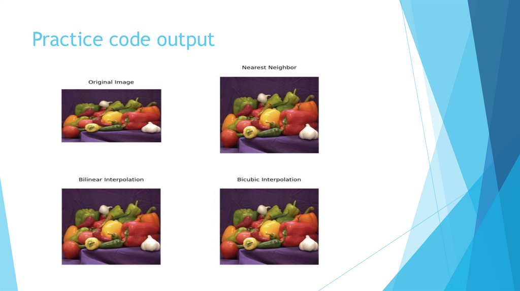
Practice code output

32.

Image Scaling
Enlarging image: Magnification, scaling up, zooming,
up-sampling, stretching.
Reducing image: Shrinking, scaling down, decimation,
down-sampling, minification
Two important things
1. Never improve upon the original image resolution
2. The resulting image will degrade with every operation

33.

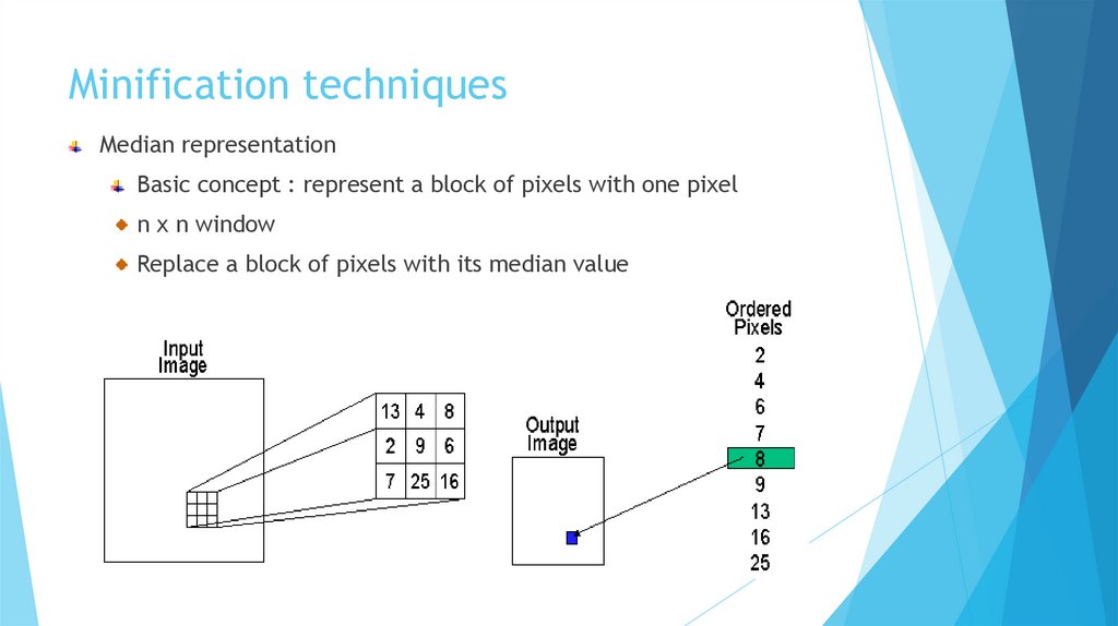
Minification techniques
Median representation
Basic concept : represent a block of pixels with one pixel
n x n window
Replace a block of pixels with its median value

34.

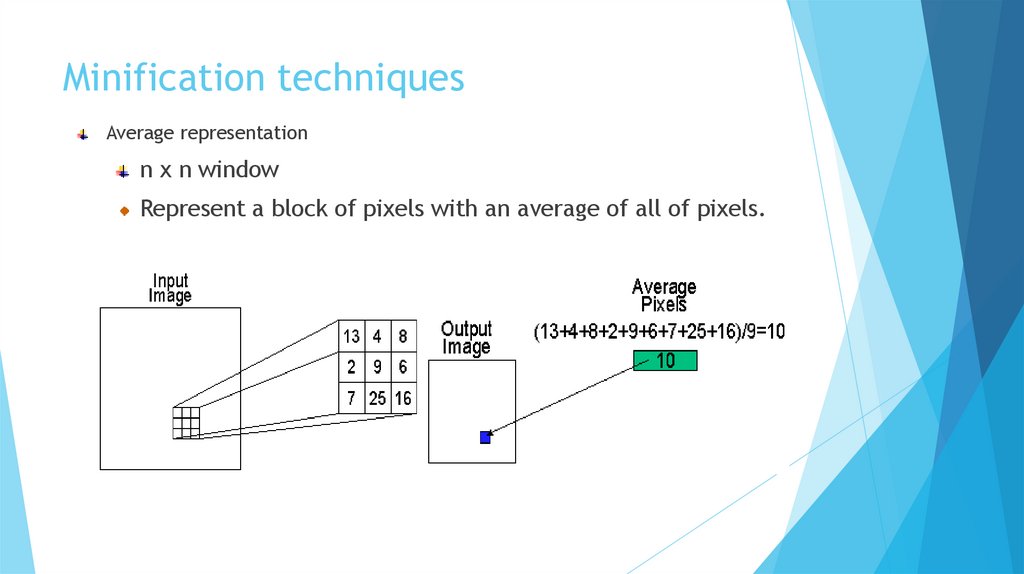
Minification techniques
Average representation
n x n window
Represent a block of pixels with an average of all of pixels.

35.

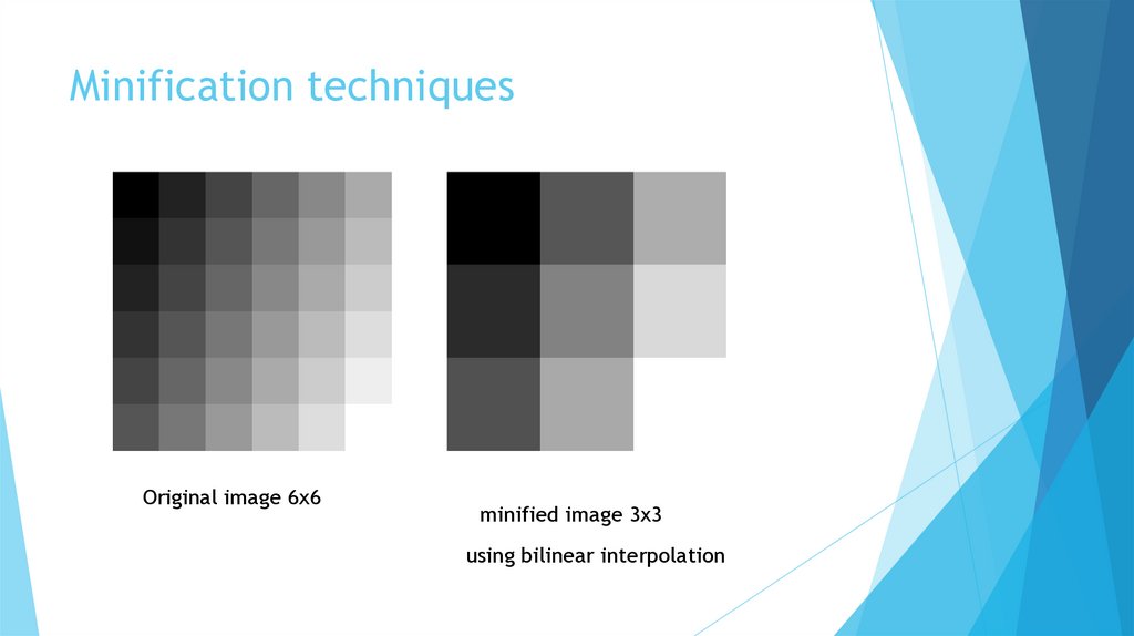
Minification techniques
Original image 6x6
minified image 3x3
using bilinear interpolation

36.

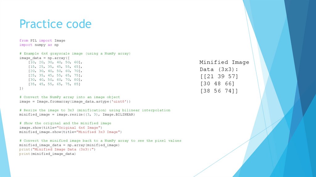
Practice code
from PIL import Image
import numpy as np
# Example 6x6 grayscale image (using a NumPy array)
image_data = np.array([
[10, 20, 30, 40, 50, 60],
[15, 25, 35, 45, 55, 65],
[20, 30, 40, 50, 60, 70],
[25, 35, 45, 55, 65, 75],
[30, 40, 50, 60, 70, 80],
[35, 45, 55, 65, 75, 85]
])
# Convert the NumPy array into an image object
image = Image.fromarray(image_data.astype('uint8'))
# Resize the image to 3x3 (minification) using bilinear interpolation
minified_image = image.resize((3, 3), Image.BILINEAR)
# Show the original and the minified image
image.show(title="Original 6x6 Image")
minified_image.show(title="Minified 3x3 Image")
# Convert the minified image back to a NumPy array to see the pixel values
minified_image_data = np.array(minified_image)
print("Minified Image Data (3x3):")
print(minified_image_data)
Minified Image
Data (3x3):
[[21 39 57]
[30 48 66]
[38 56 74]]

37.

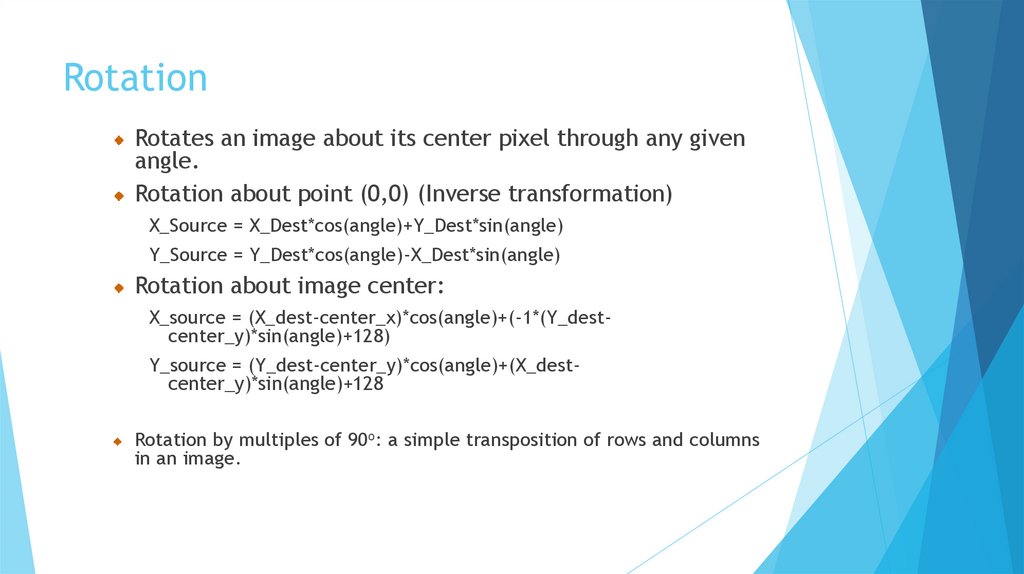
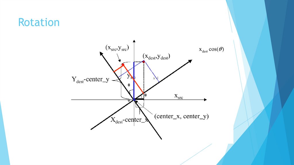
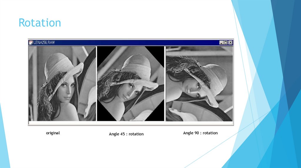
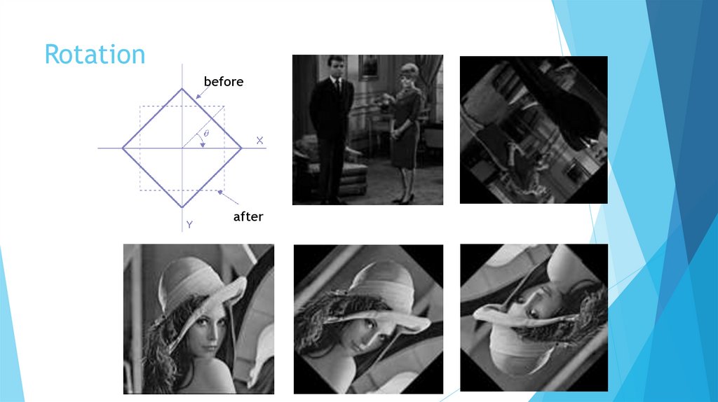
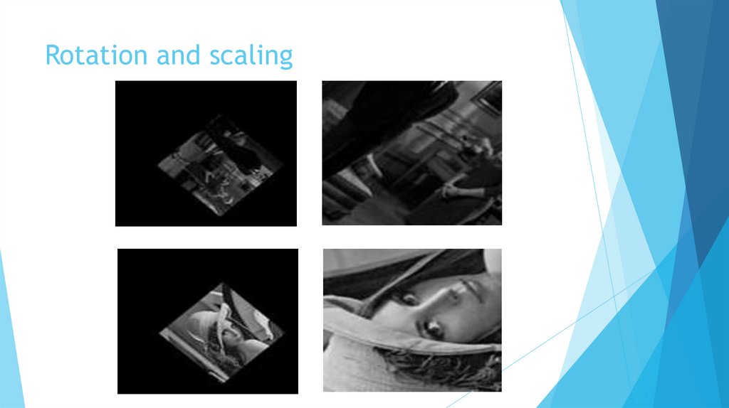
Rotation
Rotates an image about its center pixel through any given
angle.
Rotation about point (0,0) (Inverse transformation)
X_Source = X_Dest*cos(angle)+Y_Dest*sin(angle)
Y_Source = Y_Dest*cos(angle)-X_Dest*sin(angle)
Rotation about image center:
X_source = (X_dest-center_x)*cos(angle)+(-1*(Y_destcenter_y)*sin(angle)+128)
Y_source = (Y_dest-center_y)*cos(angle)+(X_destcenter_y)*sin(angle)+128
Rotation by multiples of 90o: a simple transposition of rows and columns
in an image.

38.

Rotation

39.

Rotation
original
Angle 45 : rotation
Angle 90 : rotation

40.

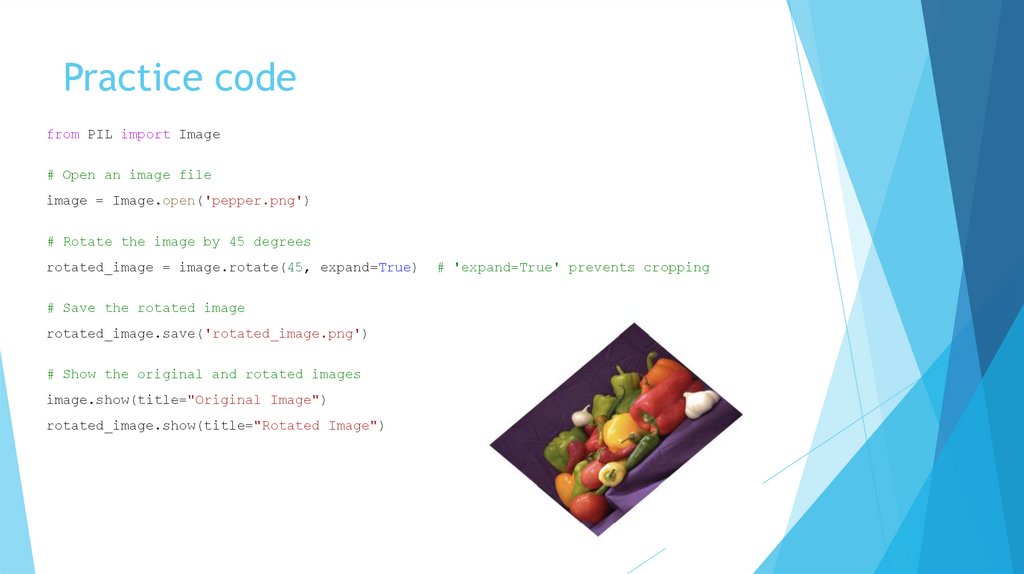
Practice code
from PIL import Image
# Open an image file
image = Image.open('pepper.png')
# Rotate the image by 45 degrees
rotated_image = image.rotate(45, expand=True)
# Save the rotated image
rotated_image.save('rotated_image.png')
# Show the original and rotated images
image.show(title="Original Image")
rotated_image.show(title="Rotated Image")
# 'expand=True' prevents cropping

41.

Rotation
before
after
41

42.

Rotation and scaling

43.

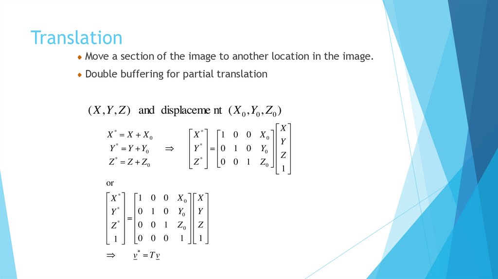
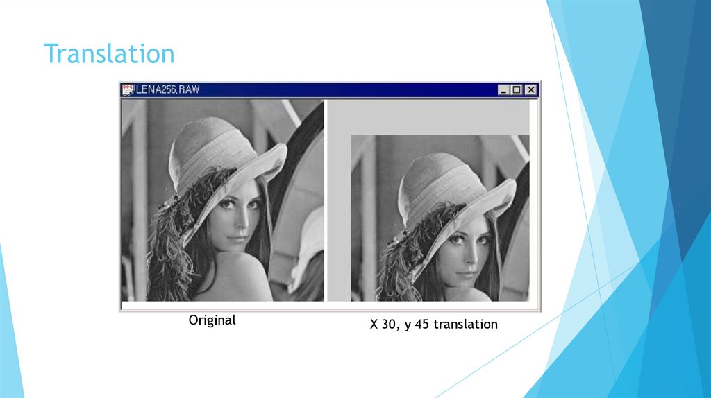
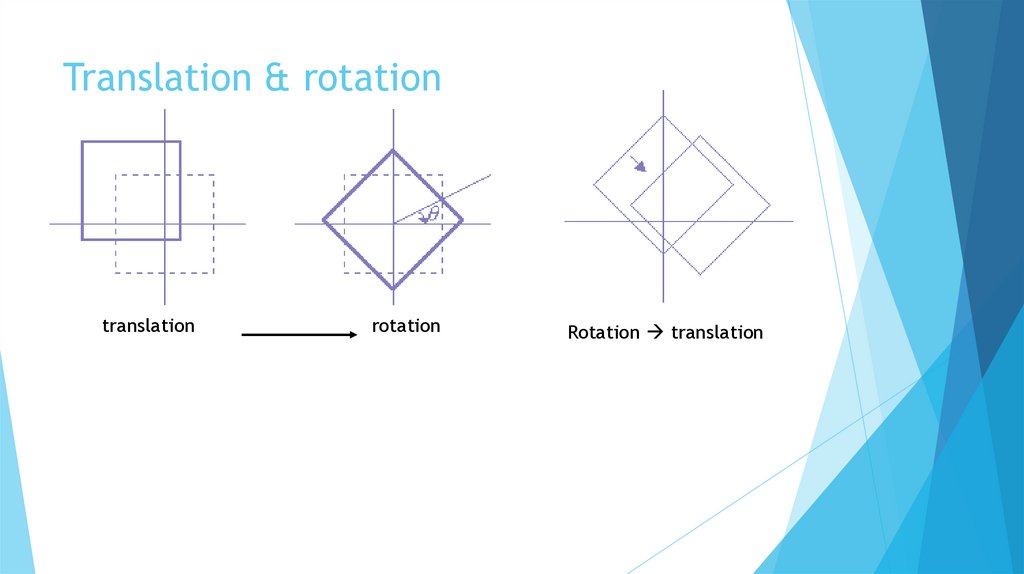
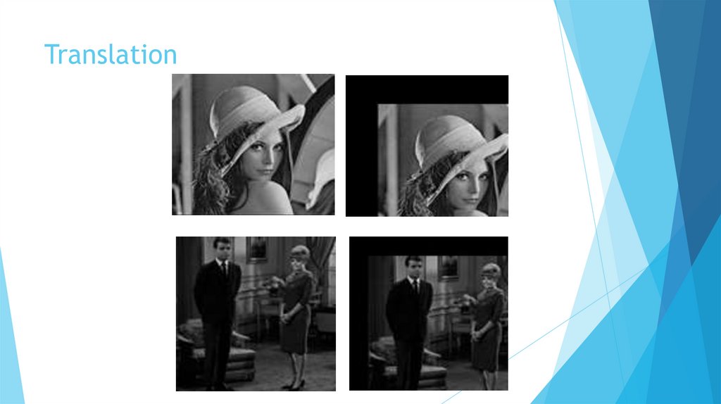
Translation
Move a section of the image to another location in the image.
Double buffering for partial translation
( X , Y , Z ) and displaceme nt ( X 0 , Y0 , Z 0 )
X * X X0
Y * Y Y0
Z * Z Z0
X * 1 0 0
*
Y 0 1 0
Z * 0 0 1
or
X * 1
*
Y 0
Z * 0
1 0
0
1
0
0
v Tv
0
0
1
0
X0 X
Y0 Y
Z0 Z
1 1
X
X0
Y
Y0
Z
Z 0
1

44.

Translation
Original
X 30, y 45 translation

45.

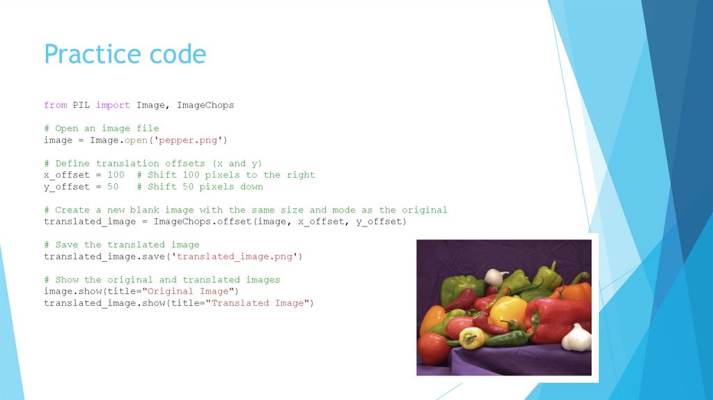
Practice code
from PIL import Image, ImageChops
# Open an image file
image = Image.open('pepper.png')
# Define translation offsets (x and y)
x_offset = 100 # Shift 100 pixels to the right
y_offset = 50
# Shift 50 pixels down
# Create a new blank image with the same size and mode as the original
translated_image = ImageChops.offset(image, x_offset, y_offset)
# Save the translated image
translated_image.save('translated_image.png')
# Show the original and translated images
image.show(title="Original Image")
translated_image.show(title="Translated Image")

46.

Translation & rotation
translation
rotation
Rotation translation

47.

Translation

48.

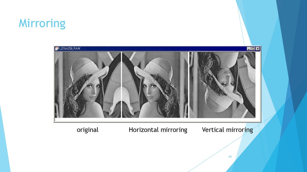
Mirroring
Flip the image about x or y axis.
Horizontal mirroring & Vertical mirroring
Pure geometric process
48

49.

Mirroring
original
Horizontal mirroring
Vertical mirroring
49

50.

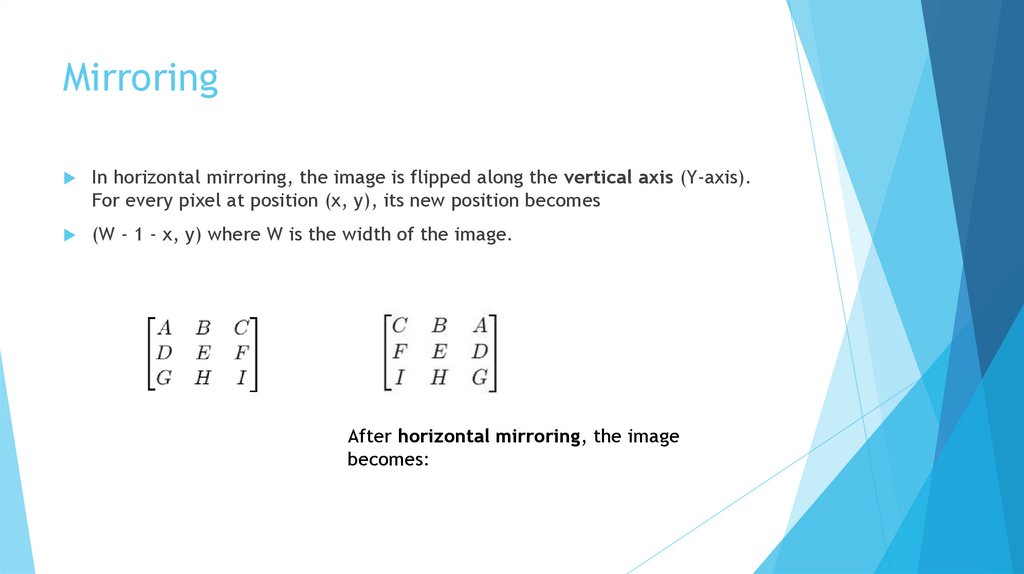
Mirroring
In horizontal mirroring, the image is flipped along the vertical axis (Y-axis).
For every pixel at position (x, y), its new position becomes
(W - 1 - x, y) where W is the width of the image.
After horizontal mirroring, the image
becomes:

51.

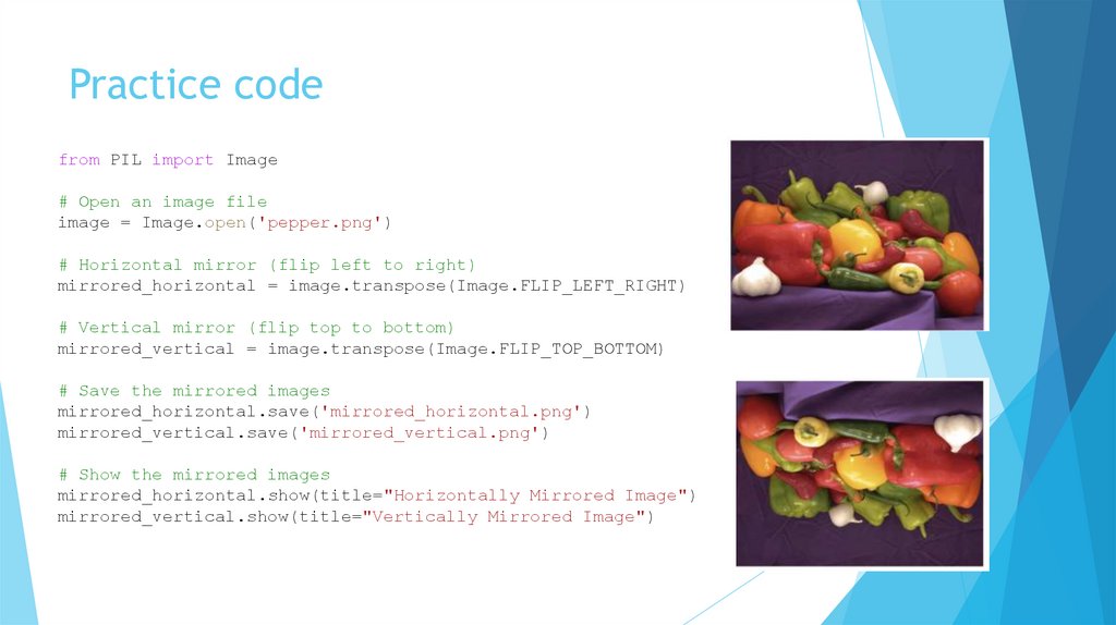
Practice code
from PIL import Image
# Open an image file
image = Image.open('pepper.png')
# Horizontal mirror (flip left to right)
mirrored_horizontal = image.transpose(Image.FLIP_LEFT_RIGHT)
# Vertical mirror (flip top to bottom)
mirrored_vertical = image.transpose(Image.FLIP_TOP_BOTTOM)
# Save the mirrored images
mirrored_horizontal.save('mirrored_horizontal.png')
mirrored_vertical.save('mirrored_vertical.png')
# Show the mirrored images
mirrored_horizontal.show(title="Horizontally Mirrored Image")
mirrored_vertical.show(title="Vertically Mirrored Image")