Practical implementation of sh lighting and hdr rendering full-length

1.

Practical Implementation of SH Lighting and
HDR Rendering on PlayStation 2
Yoshiharu Gotanda
Tatsuya Shoji
Research and Development Dept. tri-Ace Inc.

2.

This slide
• includes practical examples about
– SH Lighting for the current hardware (PlayStation 2)
– HDR Rendering
– Plug-ins for 3ds max

3.

SH Lighting gives you…
• Real-time
Global
Illumination

4.

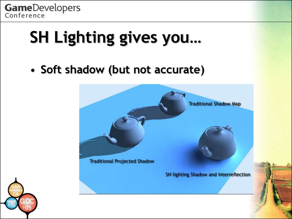
SH Lighting gives you…
• Soft shadow (but not accurate)

5.

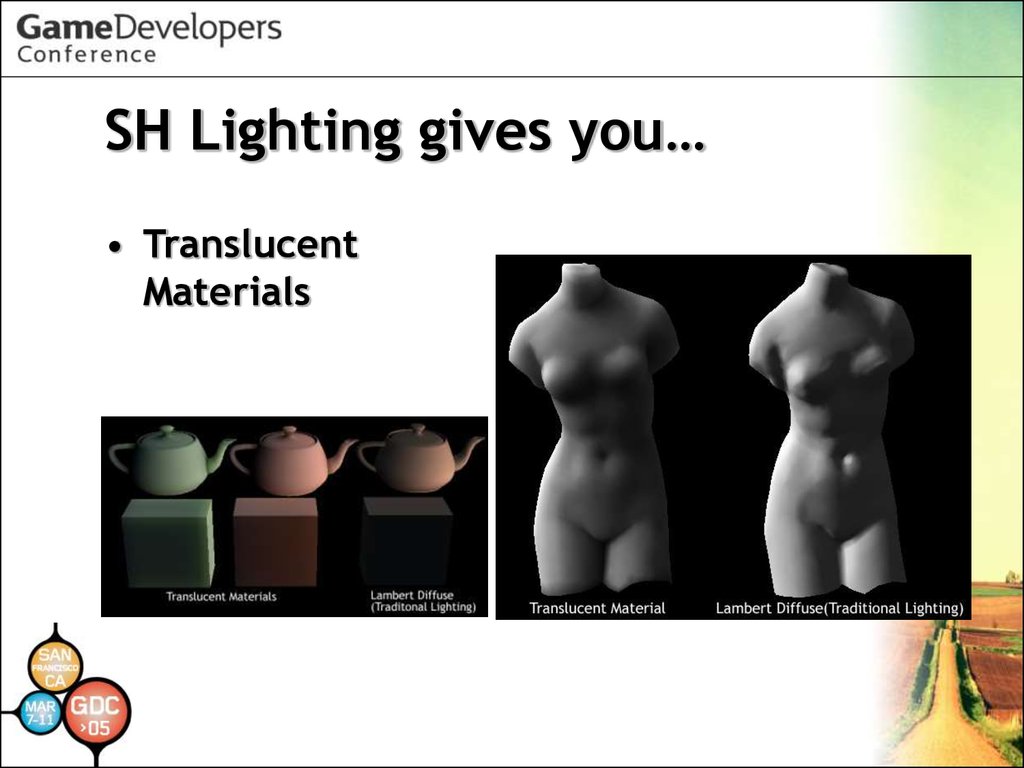
SH Lighting gives you…
• Translucent
Materials

6.

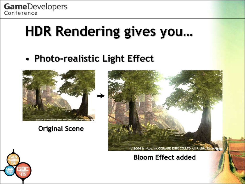
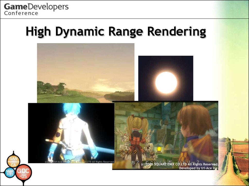
HDR Rendering gives you…
• Photo-realistic Light Effect
Original Scene
Bloom Effect added

7.

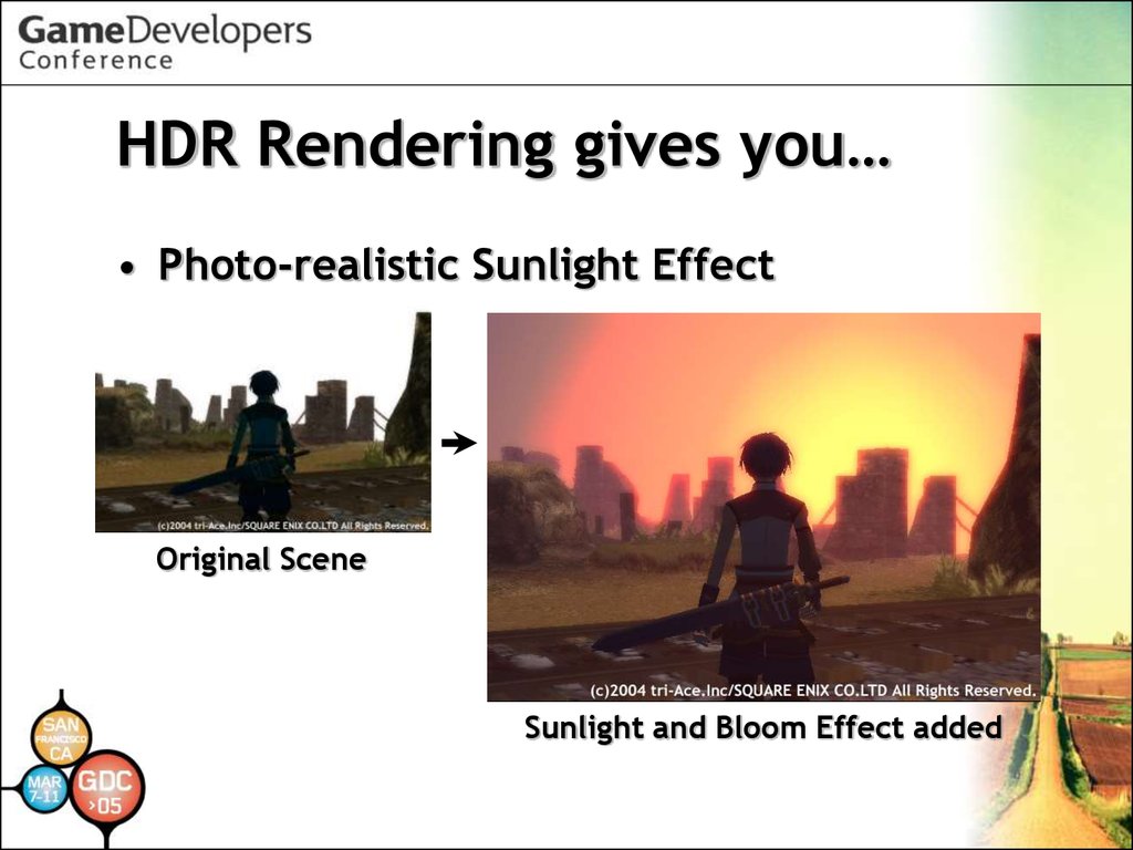
HDR Rendering gives you…
• Photo-realistic Sunlight Effect
Original Scene
Sunlight and Bloom Effect added

8.

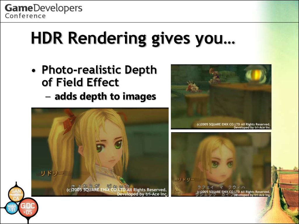
HDR Rendering gives you…
• Photo-realistic Depth
of Field Effect
– adds depth to images

9.

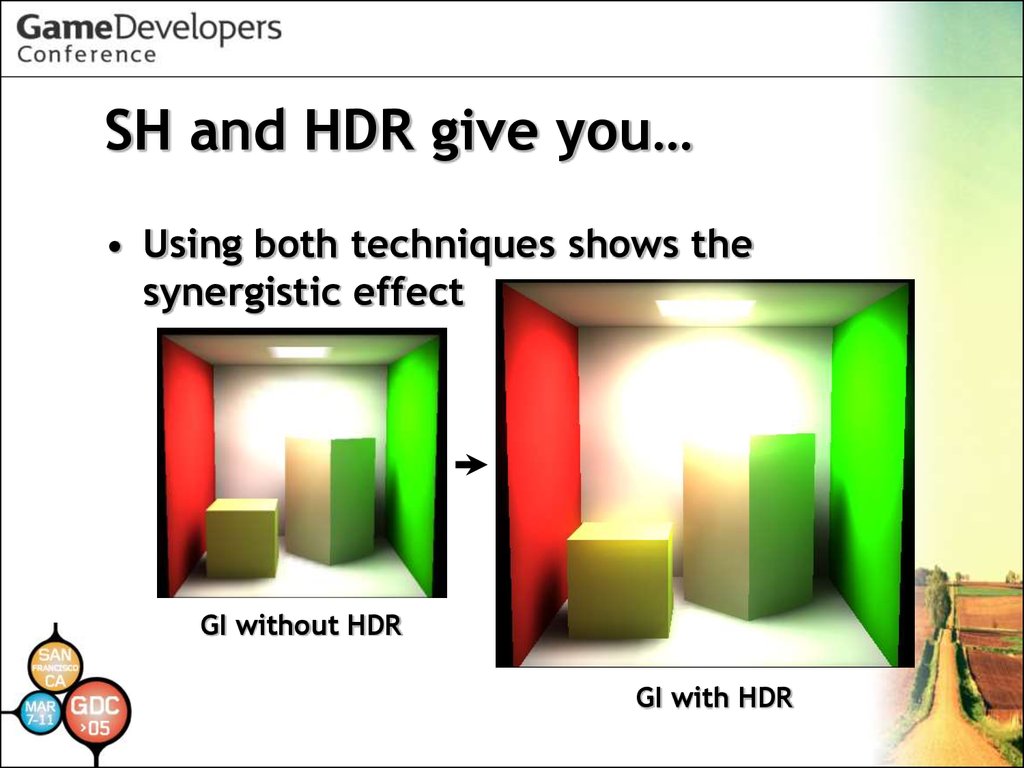
SH and HDR give you…
• Using both techniques shows the
synergistic effect
GI without HDR
GI with HDR

10.

Where to use SH and HDR
• Don’t have to use all of them
– SH lighting could be used to represent
various light phenomena
– HDR Rendering could be used to represent
various optimal phenomena as well
– There are a lot of elements (backgrounds,
characters, effects) in a game
– It is important to let artists express
themselves easily with limited resources for
each element

11.

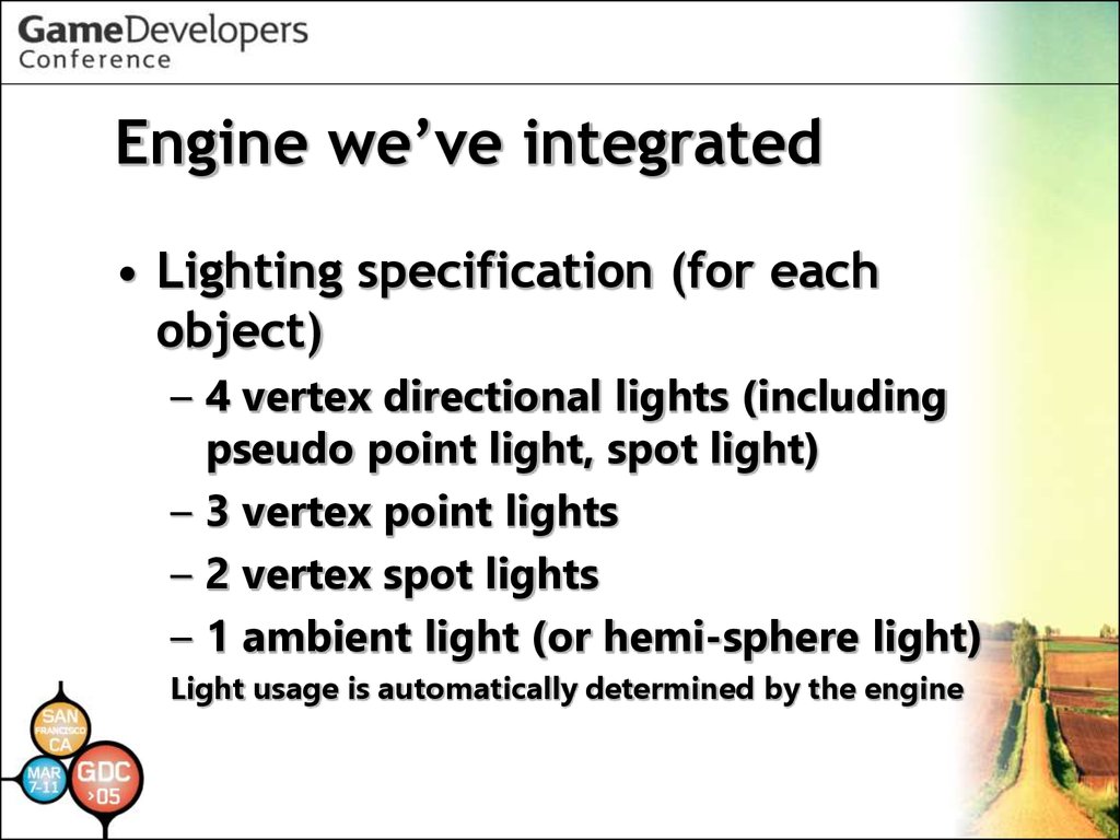
Engine we’ve integrated
• Lighting specification (for each
object)
– 4 vertex directional lights (including
pseudo point light, spot light)
– 3 vertex point lights
– 2 vertex spot lights
– 1 ambient light (or hemi-sphere light)
Light usage is automatically determined by the engine

12.

Engine we’ve integrated
• Lighting Shaders
– Color Rate Shader (light with
intensity only)
– Lambert Shader
– Phong Shader

13.

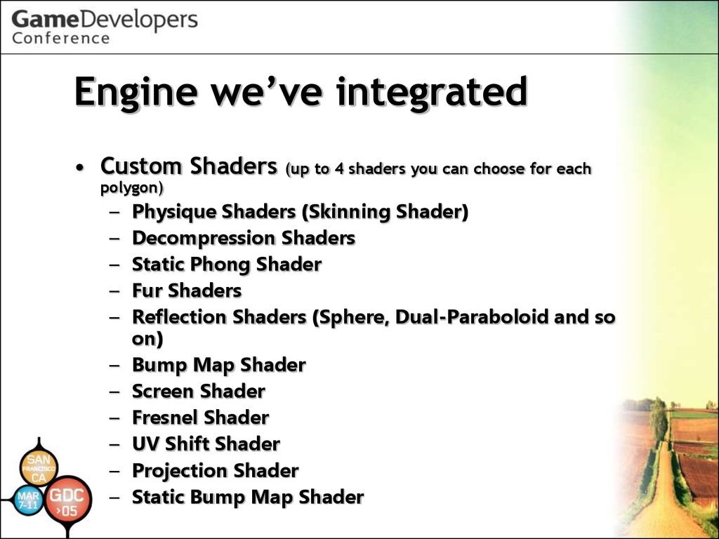
Engine we’ve integrated
• Custom Shaders
(up to 4 shaders you can choose for each
polygon)
–
–
–
–
–
–
–
–
–
–
–
Physique Shaders (Skinning Shader)
Decompression Shaders
Static Phong Shader
Fur Shaders
Reflection Shaders (Sphere, Dual-Paraboloid and so
on)
Bump Map Shader
Screen Shader
Fresnel Shader
UV Shift Shader
Projection Shader
Static Bump Map Shader

14.

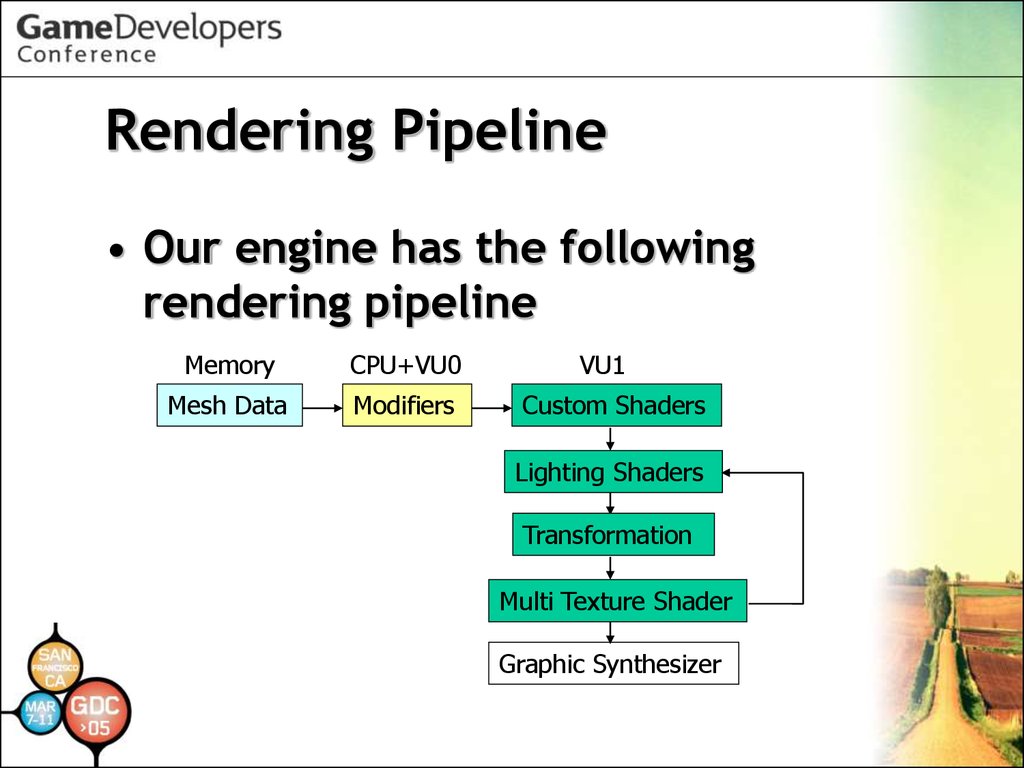
Rendering Pipeline
• Our engine has the following
rendering pipeline
Memory
CPU+VU0
Mesh Data
Modifiers
VU1
Custom Shaders
Lighting Shaders
Transformation
Multi Texture Shader
Graphic Synthesizer

15.

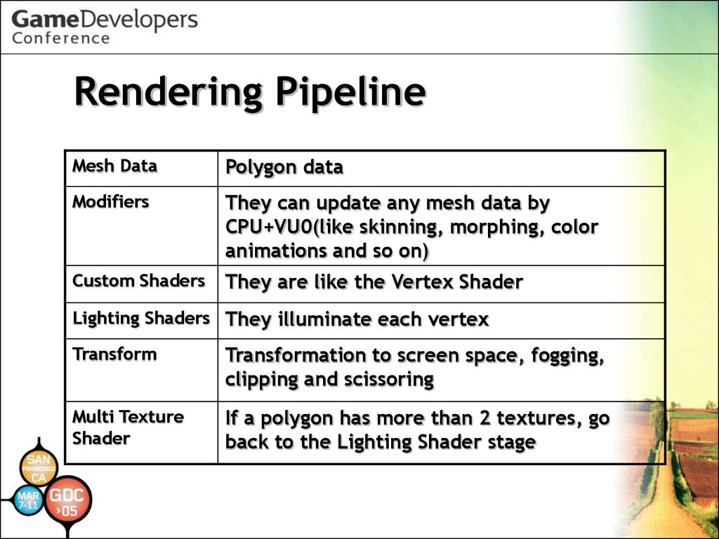
Rendering Pipeline
Mesh Data
Polygon data
Modifiers
They can update any mesh data by
CPU+VU0(like skinning, morphing, color
animations and so on)
Custom Shaders
They are like the Vertex Shader
Lighting Shaders They illuminate each vertex
Transform
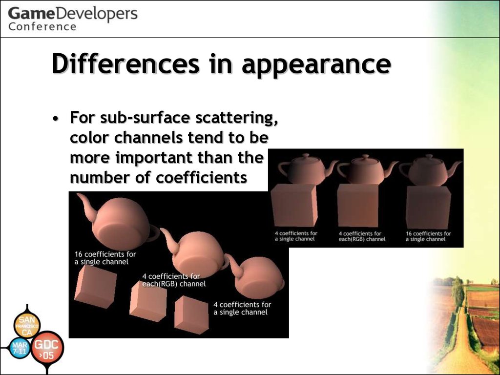
Transformation to screen space, fogging,
clipping and scissoring
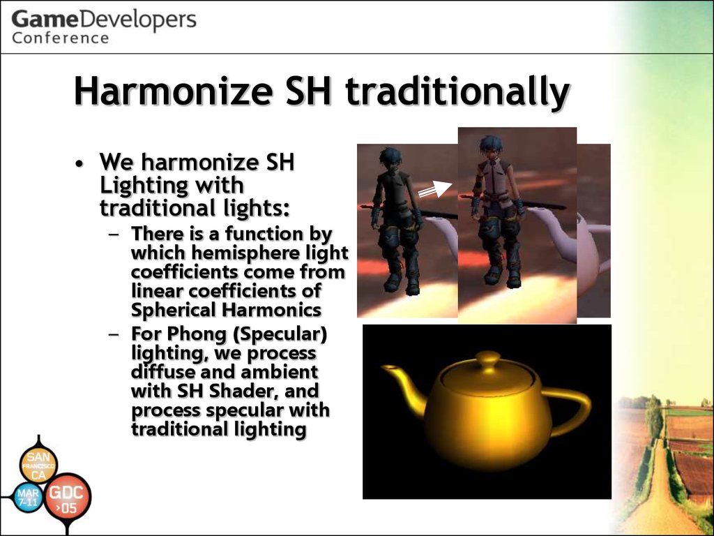
Multi Texture
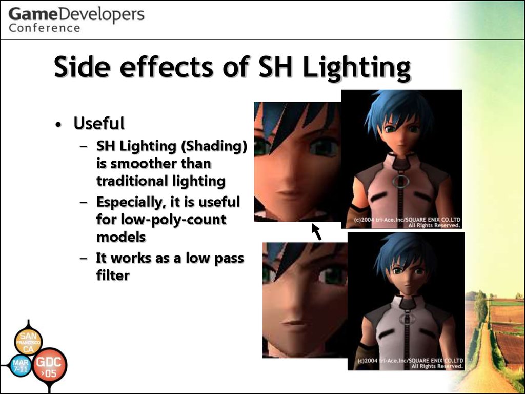
Shader
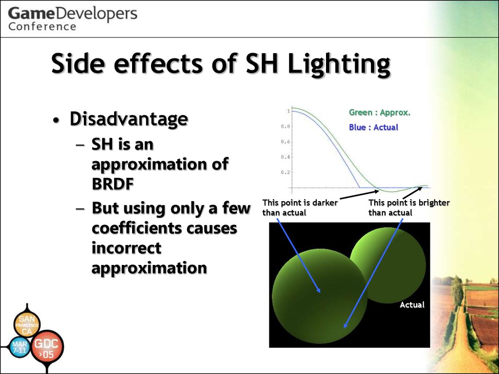
If a polygon has more than 2 textures, go
back to the Lighting Shader stage

16.

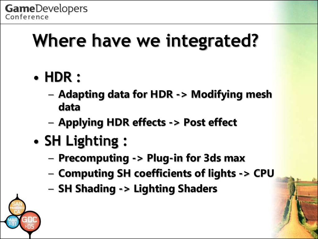
Where have we integrated?
• HDR :
– Adapting data for HDR -> Modifying mesh
data
– Applying HDR effects -> Post effect
• SH Lighting :
– Precomputing -> Plug-in for 3ds max
– Computing SH coefficients of lights -> CPU
– SH Shading -> Lighting Shaders

17.

High Dynamic Range Rendering

18.

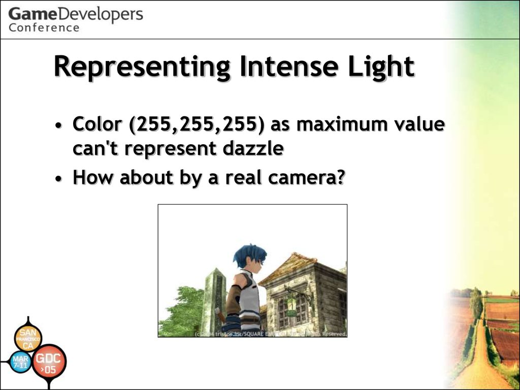
Representing Intense Light
• Color (255,255,255) as maximum value
can't represent dazzle
• How about by a real camera?

19.

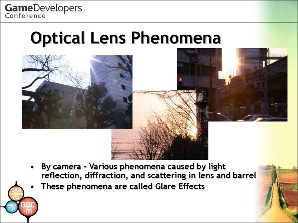
Optical Lens Phenomena
• By camera - Various phenomena caused by light
reflection, diffraction, and scattering in lens and barrel
• These phenomena are called Glare Effects

20.

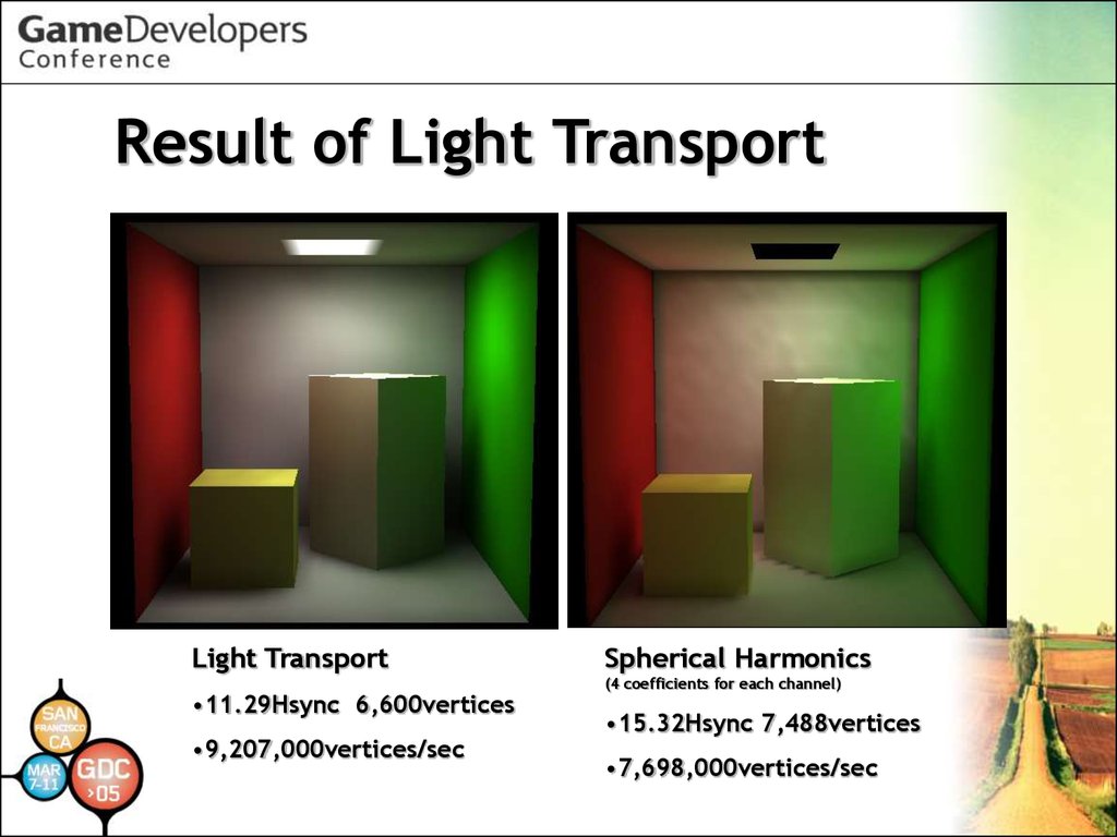
Glare Effects
• Visible only when intense light
enters
• May occur at any time but are
usually invisible when indirect
from light sources because of
faintness

21.

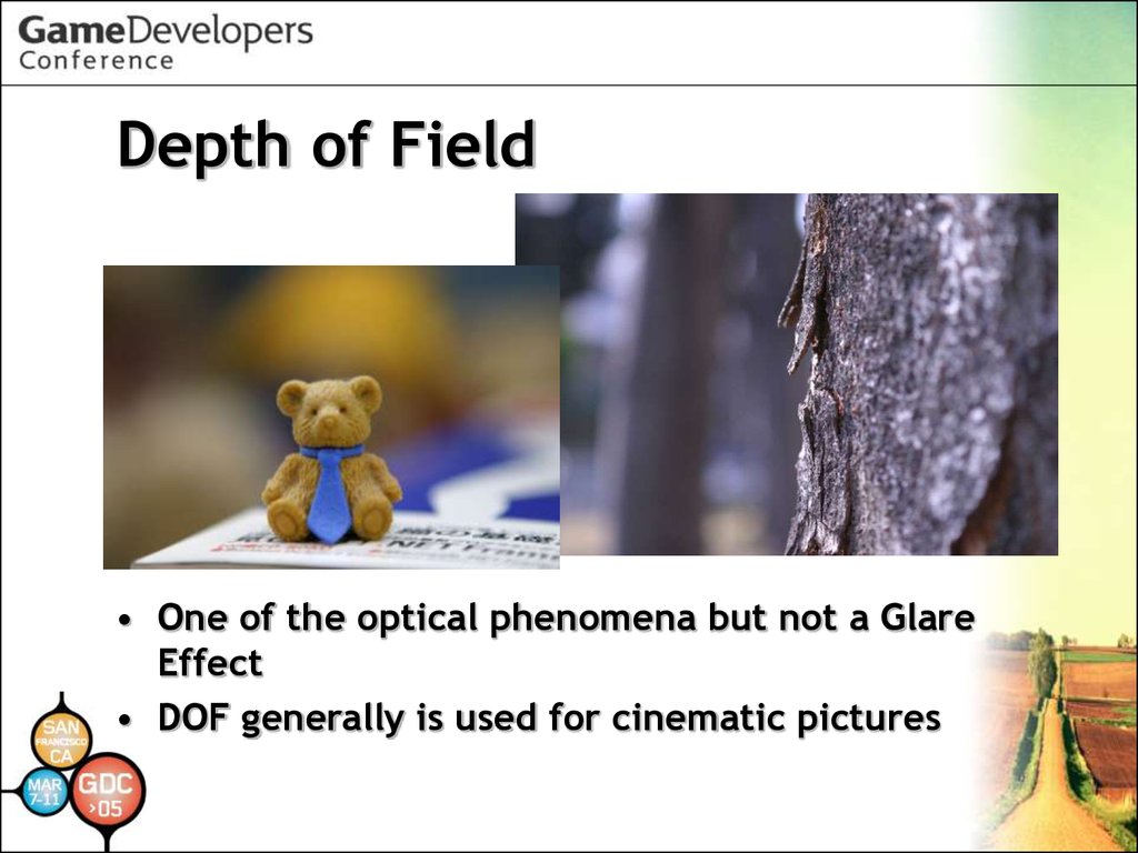
Depth of Field
• One of the optical phenomena but not a Glare
Effect
• DOF generally is used for cinematic pictures

22.

Representing Intense Light
- Bottom Line
• Accurate reproduction of Glare Effects creates
realistic intense light representations
• Glare Effects reproduction requires highly
intense brightness level
• But the frame buffer ranges only up to 255
• Keep higher level on a separate buffer (HDR
buffer)

23.

What is HDR?
• Stands for High Dynamic Range
• Dynamic Range is the ratio between
smallest and largest signal values
• In simple terms, HDR means a greater
range of value
• So HDR Buffers can represent a wide
range of intensity

24.

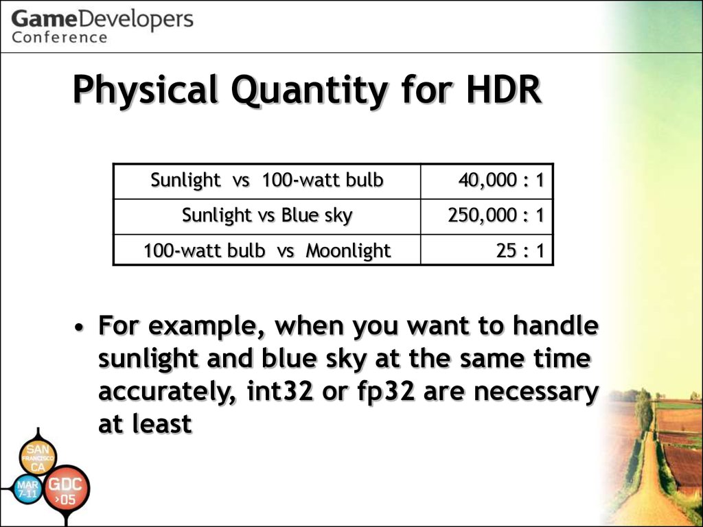
Physical Quantity for HDR
Sunlight vs 100-watt bulb
40,000 : 1
Sunlight vs Blue sky
250,000 : 1
100-watt bulb vs Moonlight
25 : 1
• For example, when you want to handle
sunlight and blue sky at the same time
accurately, int32 or fp32 are necessary
at least

25.

Implementation of HDR Buffer on PS2
• PS2 has no high precision frame buffer - Have
to utilize the 8bit-integer frame buffer
• Adopt a fixed-point-like method to raise
maximum level of intensity instead of lowering
resolution
(When usual usage is described as “0:0:8",
describe it as “0:1:7" or “0:2:6" in this
method)
• Example: If representing regular white by 128,
255 can represent double intensity level of
white
• Therefore, this method is not true HDR

26.

Mach-Band Issue
• Resolution of the visible domain gets
worse and Mach-Band is emphasized
• But with texture mapping, double rate
will be feasible

27.

Mach-Band Issue
1x
2x
4x

28.

Mach-Band Issue – with Texture
1x
2x
4x

29.

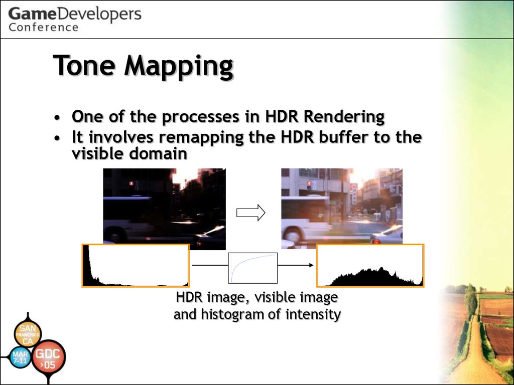
Tone Mapping
• One of the processes in HDR Rendering
• It involves remapping the HDR buffer to the
visible domain
HDR image, visible image
and histogram of intensity

30.

Tone Mapping
• Typical Tone Mapping curves are
nonlinear functions
Measurement value of digital camera (EOS 10D)
Pixel Intensity
Red
Green
Blue
Average
Fitting
Real Light Intensity

31.

Tone Mapping on PS2
• But PS2 doesn't have a pixel shader,
so simple scaling and hardware
color clamping is used

32.

Tone Mapping on PS2
• PS2's alpha blending can scale up about
six times on 1 pass
– dst = Cs*As + Cs
• Cs = FrameBuffer*2.0
• As = 2.0
• In practice, you will have a precision
problem, so use the appropriate alpha
operation:0-1x, 1-2x, 2-4x, 4-6x for
highest precision

33.

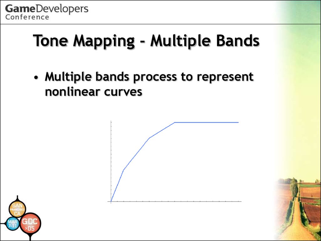
Tone Mapping - Multiple Bands
• Multiple bands process to represent
nonlinear curves

34.

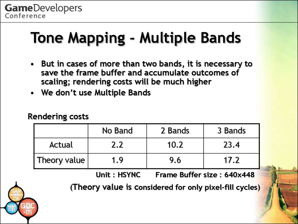
Tone Mapping - Multiple Bands
• But in cases of more than two bands, it is necessary to
save the frame buffer and accumulate outcomes of
scaling; rendering costs will be much higher
• We don’t use Multiple Bands
Rendering costs
No Band
2 Bands
3 Bands
Actual
2.2
10.2
23.4
Theory value
1.9
9.6
17.2
Unit : HSYNC
Frame Buffer size : 640x448
(Theory value is considered for only pixel-fill cycles)

35.

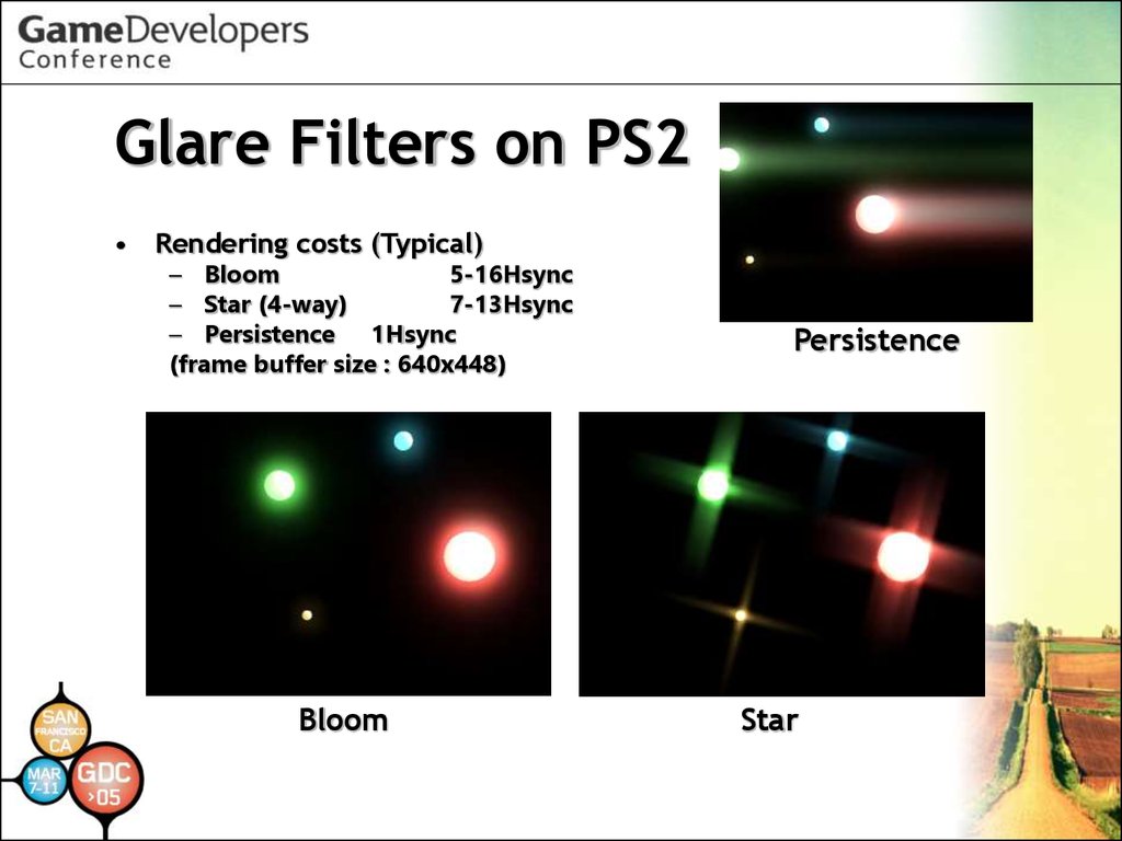
Glare Filters on PS2
• Rendering costs (Typical)
– Bloom
5-16Hsync
– Star (4-way)
7-13Hsync
– Persistence 1Hsync
(frame buffer size : 640x448)
Bloom
Persistence
Star

36.

Basic Topics for Glare Filters use
• Reduced Frame Buffer
• Filtering Threshold
• Shared Reduced Accumulation
Buffer

37.

Reduced Frame Buffer
• Using 128x128 Reduced Frame Buffer
• All processes substitute this for the
original frame buffer
• The most important tip is to reduce to
half repeatedly with bilinear filtering to
make the pixels contain average values
of the original pixels
• It will improve aliasing when a camera
or objects are in motion

38.

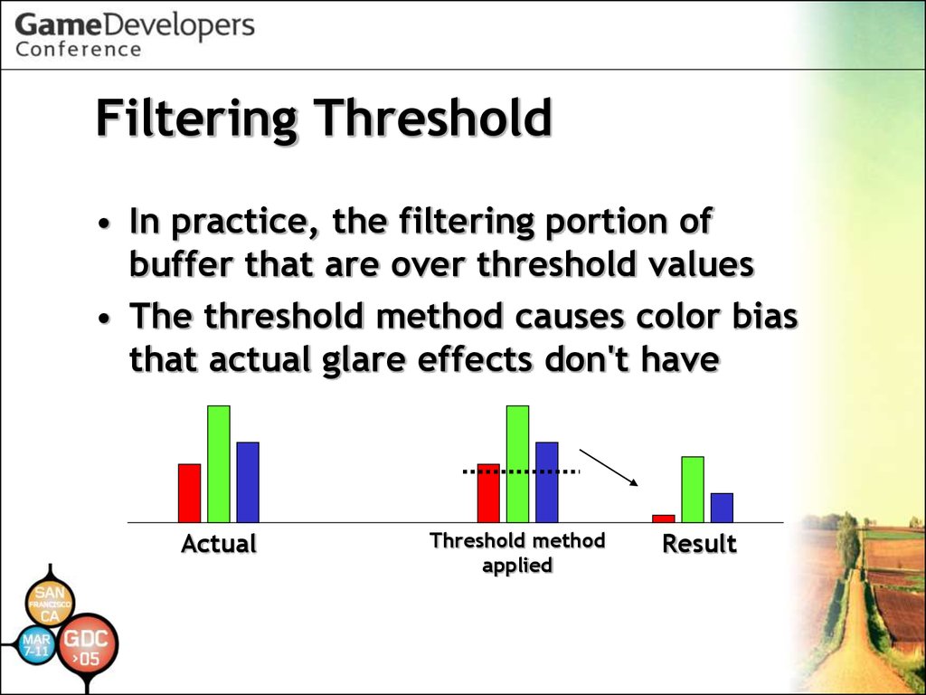
Filtering Threshold
• In practice, the filtering portion of
buffer that are over threshold values
• The threshold method causes color bias
that actual glare effects don't have
Actual
Threshold method
applied
Result

39.

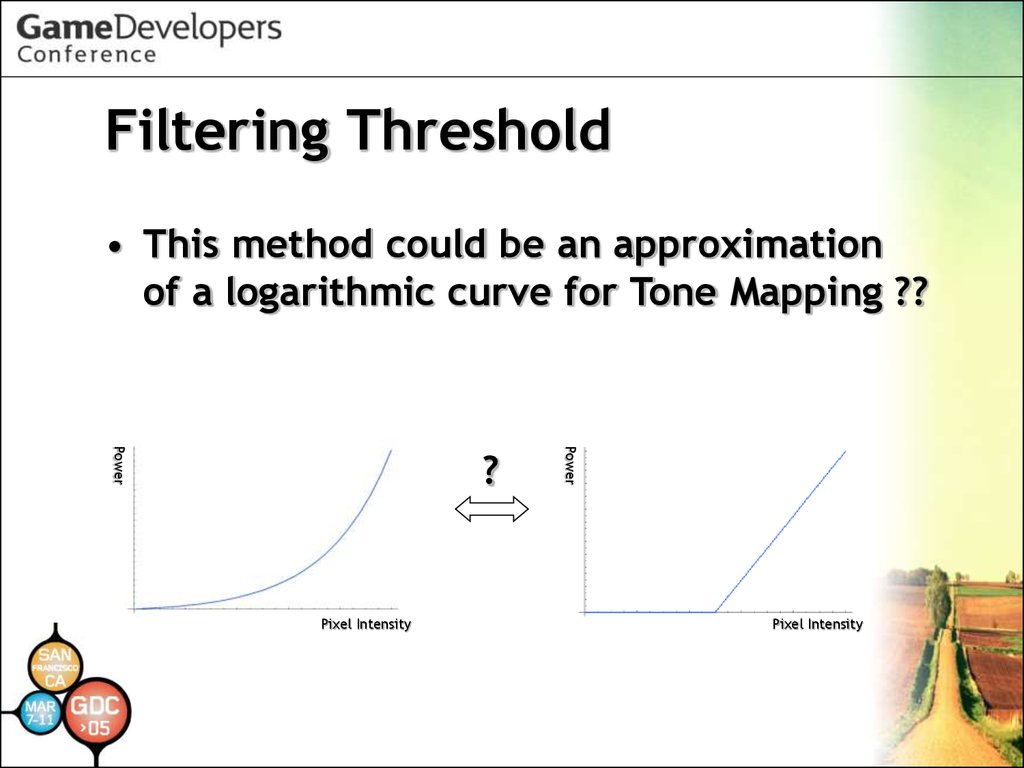
Filtering Threshold
• This method could be an approximation
of a logarithmic curve for Tone Mapping ??
Pixel Intensity
Power
Power
?
Pixel Intensity

40.

Shared Reduced ACC Buffer
• Main frame buffers take a large
area so fill costs are expensive
• Use the Shared Reduced
Accumulation Buffer to streamline
the main frame buffer once

41.

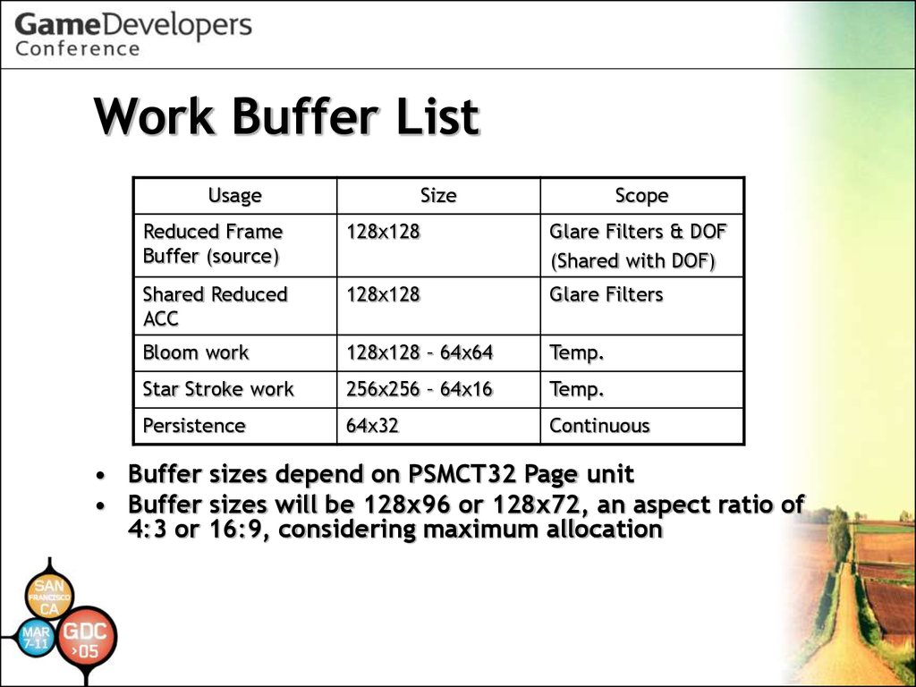
Work Buffer List
Usage
Size
Scope
Reduced Frame
Buffer (source)
128x128
Glare Filters & DOF
(Shared with DOF)
Shared Reduced
ACC
128x128
Glare Filters
Bloom work
128x128 – 64x64
Temp.
Star Stroke work
256x256 – 64x16
Temp.
Persistence
64x32
Continuous
• Buffer sizes depend on PSMCT32 Page unit
• Buffer sizes will be 128x96 or 128x72, an aspect ratio of
4:3 or 16:9, considering maximum allocation

42.

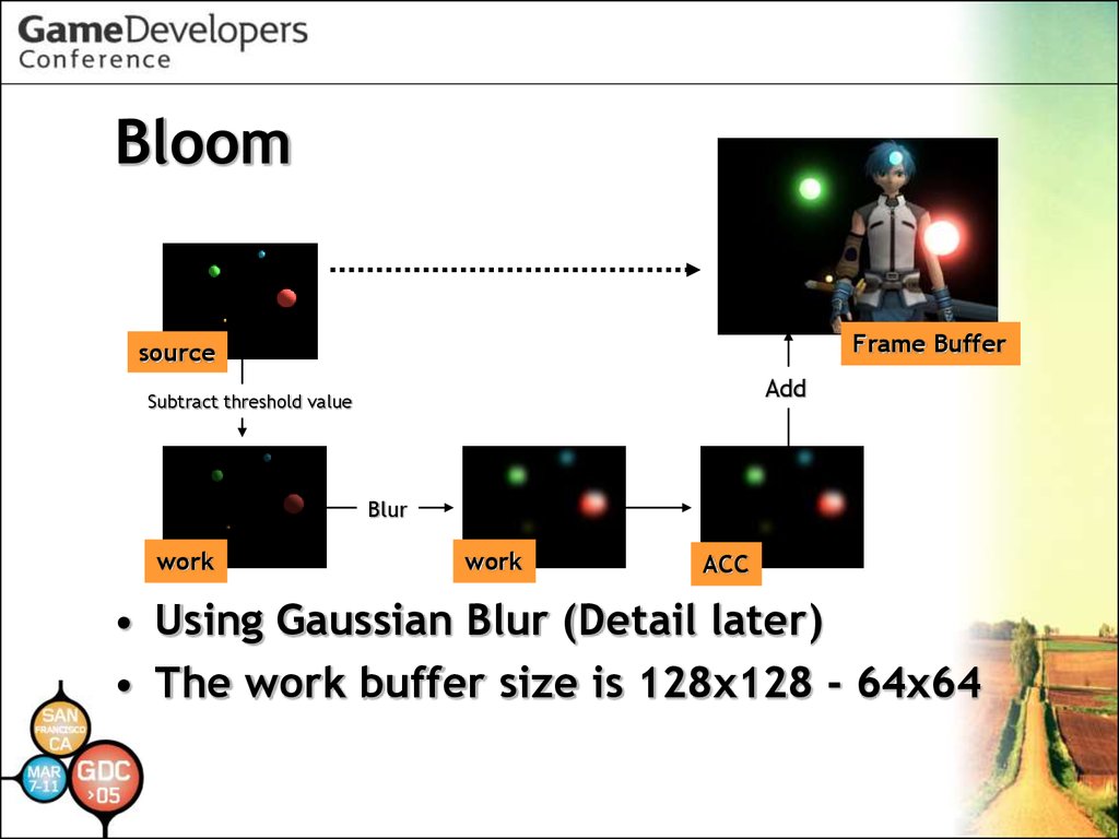
Bloom
Frame Buffer
source
Add
Subtract threshold value
Blur
work
work
ACC
• Using Gaussian Blur (Detail later)
• The work buffer size is 128x128 - 64x64

43.

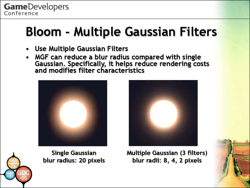
Bloom - Multiple Gaussian Filters
• Use Multiple Gaussian Filters
• MGF can reduce a blur radius compared with single
Gaussian. Specifically, it helps reduce rendering costs
and modifies filter characteristics
Single Gaussian
blur radius: 20 pixels
Multiple Gaussian (3 filters)
blur radii: 8, 4, 2 pixels

44.

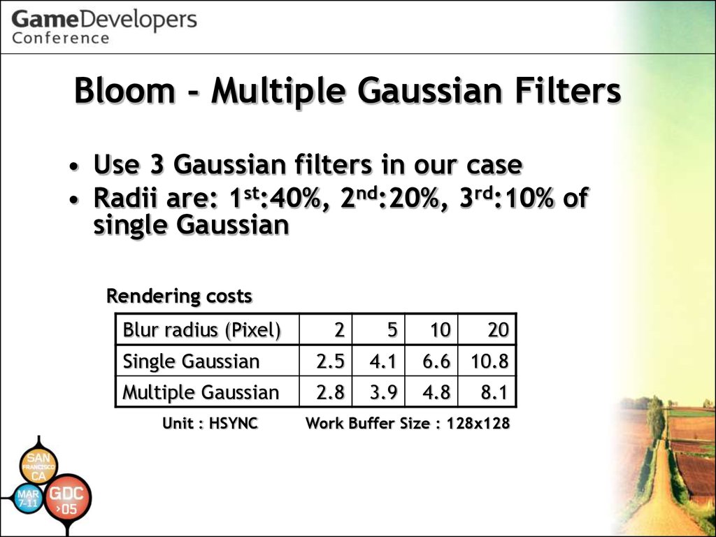
Bloom - Multiple Gaussian Filters
• Use 3 Gaussian filters in our case
• Radii are: 1st:40%, 2nd:20%, 3rd:10% of
single Gaussian
Rendering costs
Blur radius (Pixel)
2
5
Single Gaussian
2.5
4.1
6.6 10.8
Multiple Gaussian
2.8
3.9
4.8
Unit : HSYNC
10
20
8.1
Work Buffer Size : 128x128

45.

Star
Frame Buffer
work
ACC
source
1st pass
Create stroke
….
….
Rotate and
compress
Unrotate
and stretch
• Create each stroke on the work buffer and then
accumulate it on the ACC Buffer
• Use a non-square work buffer that is reduced in the
stroke's direction to save taps of stroke creation
• Vary buffer height in order to fix the tap count
4th pass

46.

Star Issue
• Can't draw sharp edges on Reduced
ACC buffer
• Copying directly from a work
buffer to the main frame buffer
can improve quality
• But fill costs will increase

47.

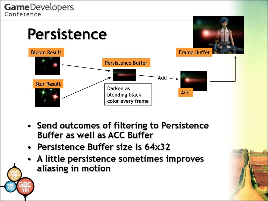
Persistence
Bloom Result
Frame Buffer
Persistence Buffer
Add
Star Result
Darken as
blending black
color every frame
ACC
• Send outcomes of filtering to Persistence
Buffer as well as ACC Buffer
• Persistence Buffer size is 64x32
• A little persistence sometimes improves
aliasing in motion

48.

More Details for Glare Filters
• Multiple Gaussian Filters
• How to create star strokes
• and so on..
See references below
– Masaki Kawase. "Frame Buffer Postprocessing Effects in
DOUBLE-S.T.E.A.L (Wreckless)“ GDC 2003.
– Masaki Kawase. "Practical Implementation of High
Dynamic Range Rendering“ GDC 2004.

49.

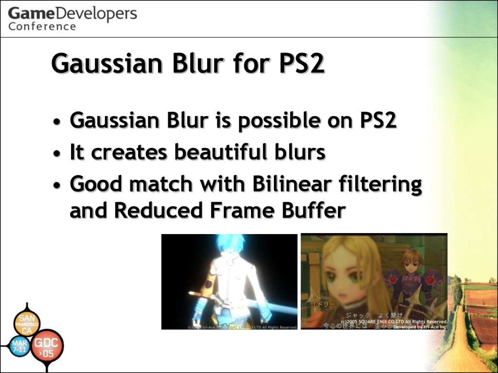
Gaussian Blur for PS2
• Gaussian Blur is possible on PS2
• It creates beautiful blurs
• Good match with Bilinear filtering
and Reduced Frame Buffer

50.

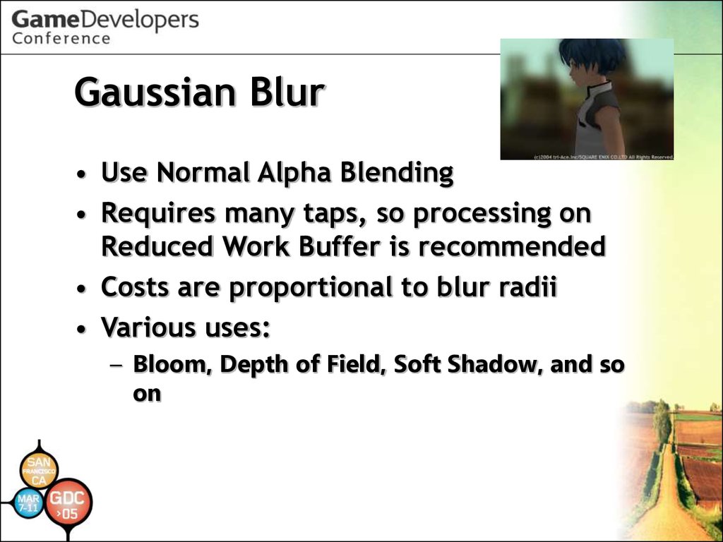
Gaussian Blur
• Use Normal Alpha Blending
• Requires many taps, so processing on
Reduced Work Buffer is recommended
• Costs are proportional to blur radii
• Various uses:
– Bloom, Depth of Field, Soft Shadow, and so
on

51.

Gaussian Filter on PS2
• Compute Normal blending
coefficients to distribute the pixel
color to nearby pixels according to
Gaussian Distribution
• Don’t use Additive Alpha Blending

52.

Gaussian Filter on PS2
Example: To distribute 25% to both sides
1st pass, blend 25% / (100%-25%)=33% to one side
2nd pass, blend 25% to the other side
1st pass, Blend 33%
Original Pixels
Shift to Left
+
255
255
2nd pass, Blend 25%
255
Shift to Right
+
85 170
255
Required Pixels
63 128 63
63 128 63
Left Pixel : ( 0*(1-0.77) + 255 * 0.33 ) * (1-0.25) + 0 * 0.25 = 63
Right Pixel : 0 * (1-0.25) + 255 * 0.25 = 63

53.

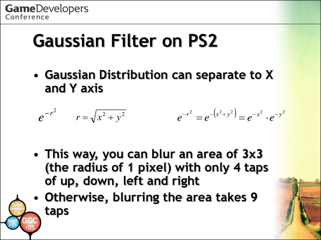
Gaussian Filter on PS2
• Gaussian Distribution can separate to X
and Y axis
e
r2
r x y
2
2
e
r 2
e
x2 y2
e x e y
2
• This way, you can blur an area of 3x3
(the radius of 1 pixel) with only 4 taps
of up, down, left and right
• Otherwise, blurring the area takes 9
taps
2

54.

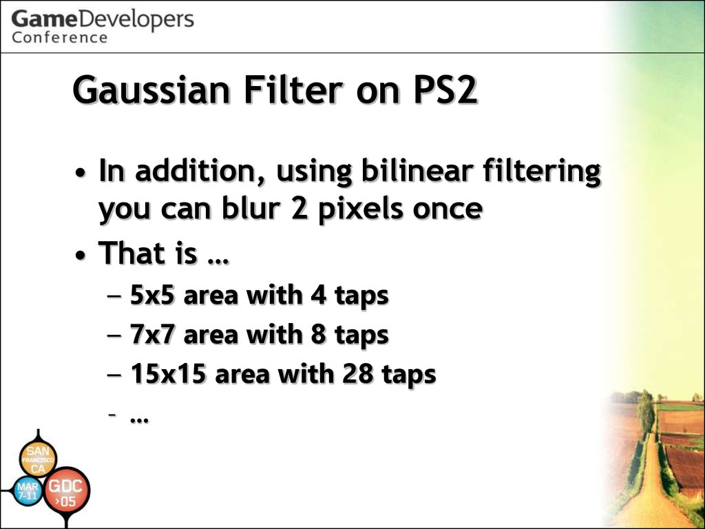
Gaussian Filter on PS2
• In addition, using bilinear filtering
you can blur 2 pixels once
• That is …
–
–
–
–
5x5 area with 4 taps
7x7 area with 8 taps
15x15 area with 28 taps
…

55.

Lack of Buffer Precision
• 8-bit integer does not have enough precision to blur a
wide radius. it can blur only about 30 pixels
• Precision in the process of calculations is preserved
when using Normal Blending, but it's not preserved when
using Additive Blending
Broken to X and Y axis
Blur radius : 40 pixels

56.

Gaussian Filter Optimization
• Of course using VU1 saves CPU
• Avoiding Destination Page Break
Penalty of a frame buffer is
effective for those filters
• In addition, avoiding Source Page
Break Penalty reduces rendering
costs by 40%

57.

Depth of Field
• Achievements of our system:
– Reasonable rendering costs:
• 8-24Hsync(typically), 35Hsync
• (frame buffer size : 640x448)
– Extreme blurs
– Accurate blur radii and handling by
real camera parameters
• Focal length and F-stop

58.

Depth of Field

59.

Depth of Field overview
+
=
• Basically, blend a frame image and a blurred
image based on alpha coefficients computed
from Z values
• Use Gaussian Filter for blurring
• Use reduced work buffers : 128x128 – 64x64

60.

Multiple Blurred Layers
• There are at most 3 layers as the background
and 2 layers as the foreground in our case
• We use Blend and Blur Masks to improve some
artifacts

61.

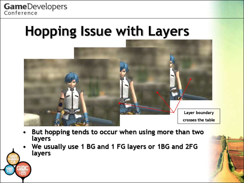
Hopping Issue with Layers
Layer boundary
crosses the table
• But hopping tends to occur when using more than two
layers
• We usually use 1 BG and 1 FG layers or 1BG and 2FG
layers

62.

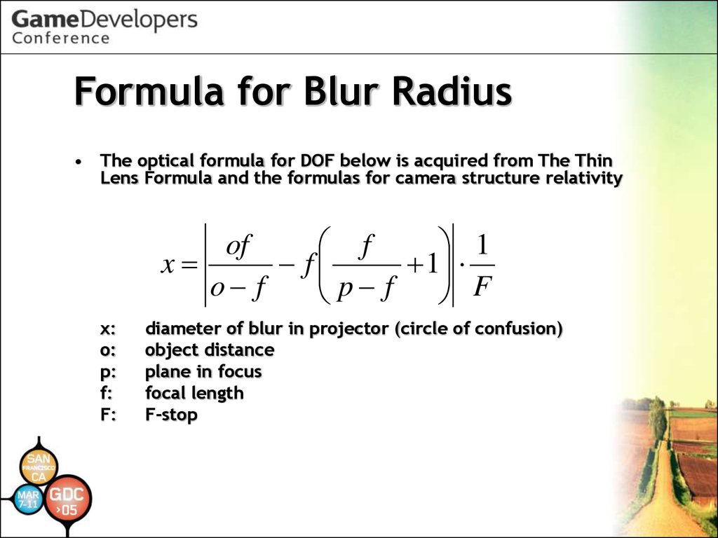
Formula for Blur Radius
• The optical formula for DOF below is acquired from The Thin
Lens Formula and the formulas for camera structure relativity
f
1
of
x
f
1
o f
p f
F
x:
o:
p:
f:
F:
diameter of blur in projector (circle of confusion)
object distance
plane in focus
focal length
F-stop

63.

Conversions of Frame Buffers
• DOF uses the conversions of frame
buffers below (details later)
– Swizzling Each Color Element from G
to A or A to G
– Converting Z to RGB with CLUT
– Shifting Z bits toward upper side

64.

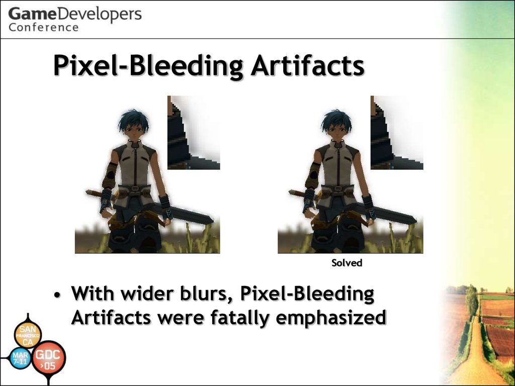
Pixel-Bleeding Artifacts
Solved
• With wider blurs, Pixel-Bleeding
Artifacts were fatally emphasized

65.

Pixel-Bleeding Artifacts
• Solve it by blurring with a mask
• Use normal alpha blending so put
masks in alpha components of a
source buffer
• Gaussian Distribution is incorrect
near the borders of the mask but
looks OK

66.

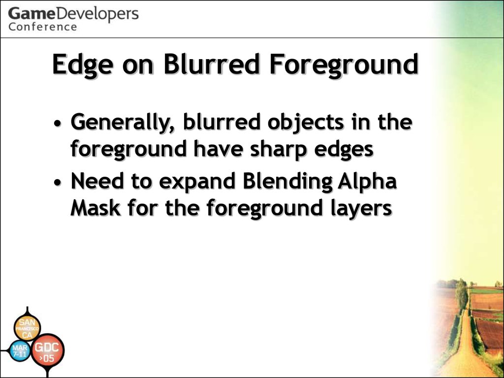
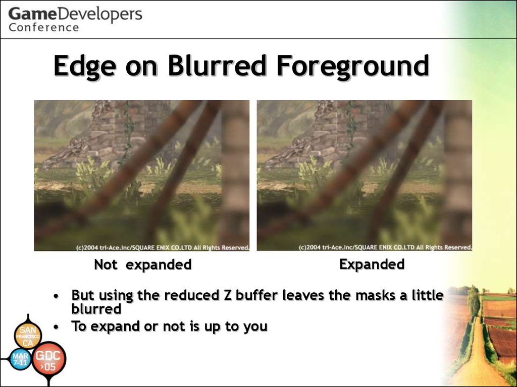
Edge on Blurred Foreground
• Generally, blurred objects in the
foreground have sharp edges
• Need to expand Blending Alpha
Mask for the foreground layers

67.

Edge on Blurred Foreground
Not expanded
Expanded
• But using the reduced Z buffer leaves the masks a little
blurred
• To expand or not is up to you

68.

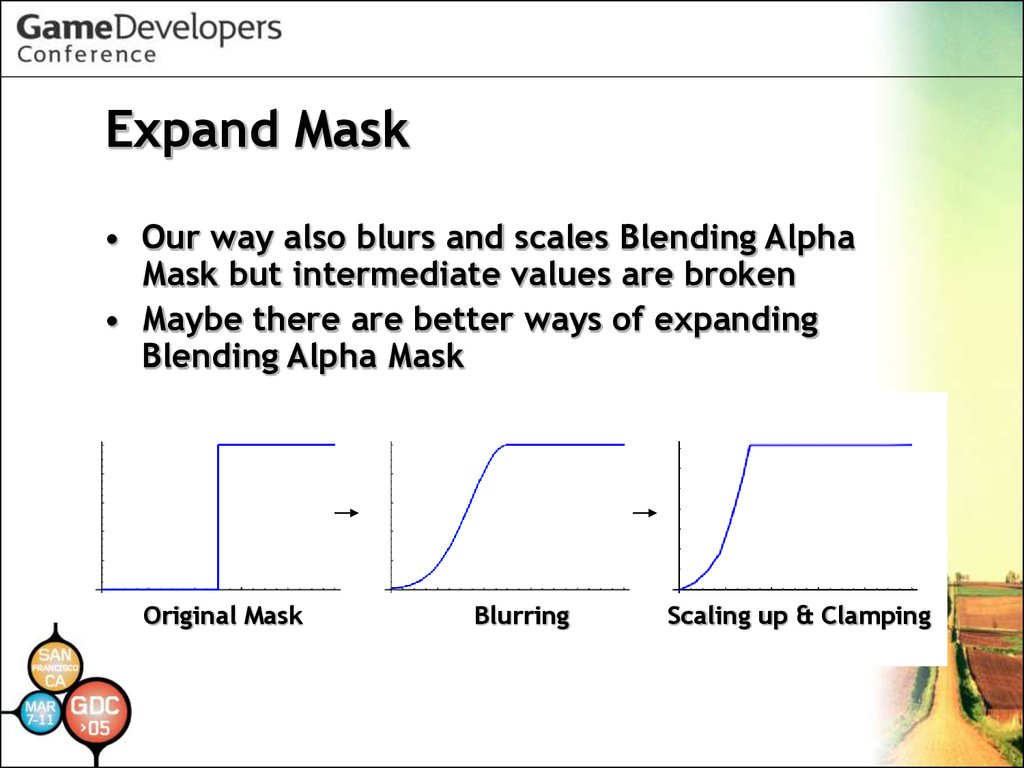
Expand Mask
• Our way also blurs and scales Blending Alpha
Mask but intermediate values are broken
• Maybe there are better ways of expanding
Blending Alpha Mask
Original Mask
Blurring
Scaling up & Clamping

69.

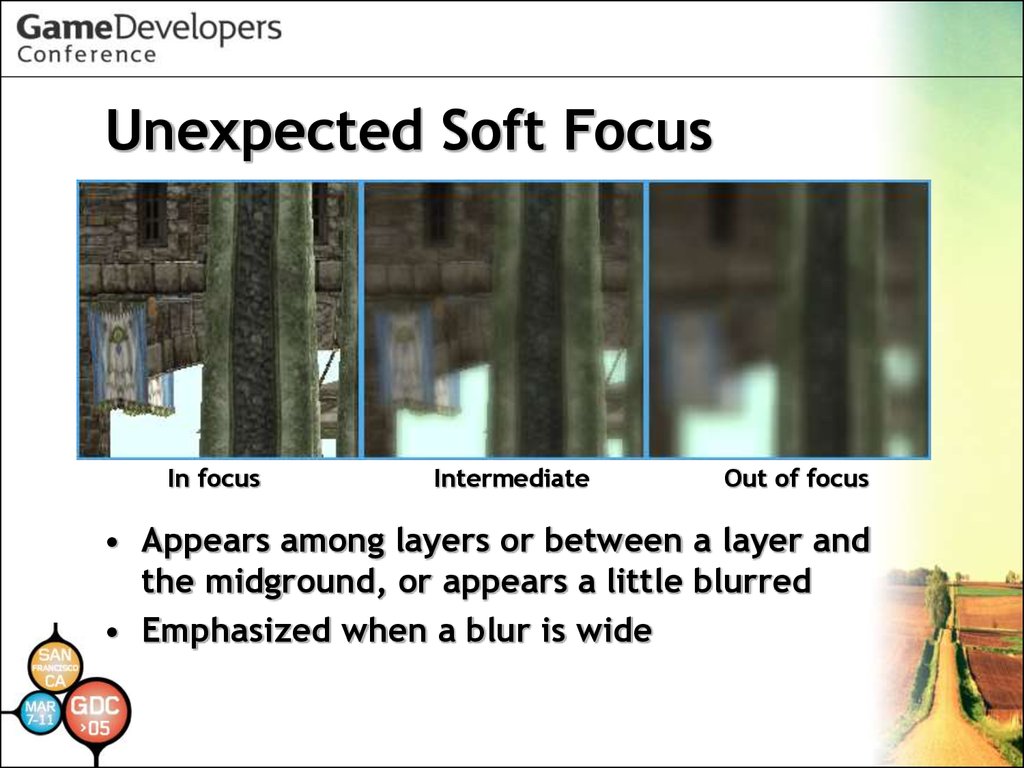
Unexpected Soft Focus
In focus
Intermediate
Out of focus
• Appears among layers or between a layer and
the midground, or appears a little blurred
• Emphasized when a blur is wide

70.

Unexpected Soft Focus
• One solution is to increase the
number of layers
• Another way is to put intermediate
values on the blurring mask
• But it causes incorrect Gaussian
blurring areas

71.

Intermediate Mask of Gaussian
With intermediate values
Regular Gaussian
The apparent difference of depth with single
layer … a little better

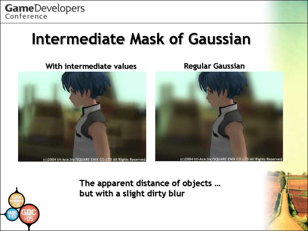
72.

Intermediate Mask of Gaussian
With intermediate values
Regular Gaussian
The apparent distance of objects …
but with a slight dirty blur

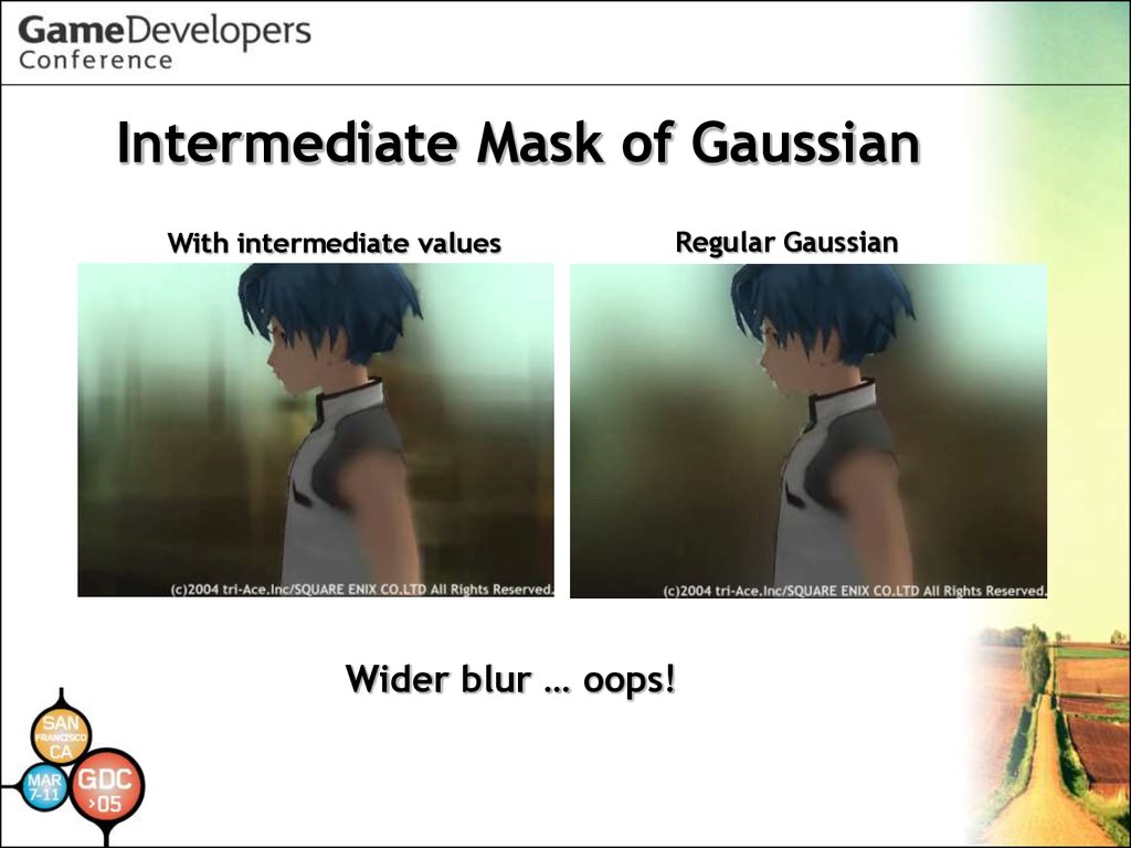
73.

Intermediate Mask of Gaussian
With intermediate values
Regular Gaussian
Wider blur … oops!

74.

Unnatural Blur
• Gaussian Function is different from
a real camera blur
• The real blur function is more flat
• Maybe the difference will be
conspicuous using HDR values

75.

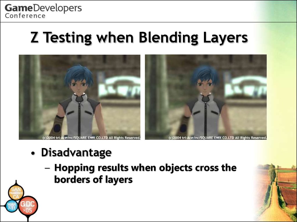
Z Testing when Blending Layers
With Z test
Without
• Advantage
– Clearer edge with a reduced Z buffer

76.

Z Testing when Blending Layers
• Disadvantage
– Hopping results when objects cross the
borders of layers

77.

Converting Flow Overview
• DOF flow
Reduced Frame Buffer
Frame Buffer Z & Color
Reduce Z
Background Layers
Foreground
Layers
Blend to Frame Buffer
Scale & Clamp
blur Frame with Mask
Shift Z bit
blur Blend Mask
CLUT Look up
Reduce Z
(Don’t Shift)
Glare
Effects
flow
Blend & Blur Mask

78.

Converting Flow Overview
• Glare Effects flow
Reduce Intensity
Reduce Intensity
Darken Every Frame
Bloom
Create Star Strokes
Persistence
Star
Copy and Rotate
Reduce size
Blur
Add to Frame
Buffer
Reduced Accumulation Buffer

79.

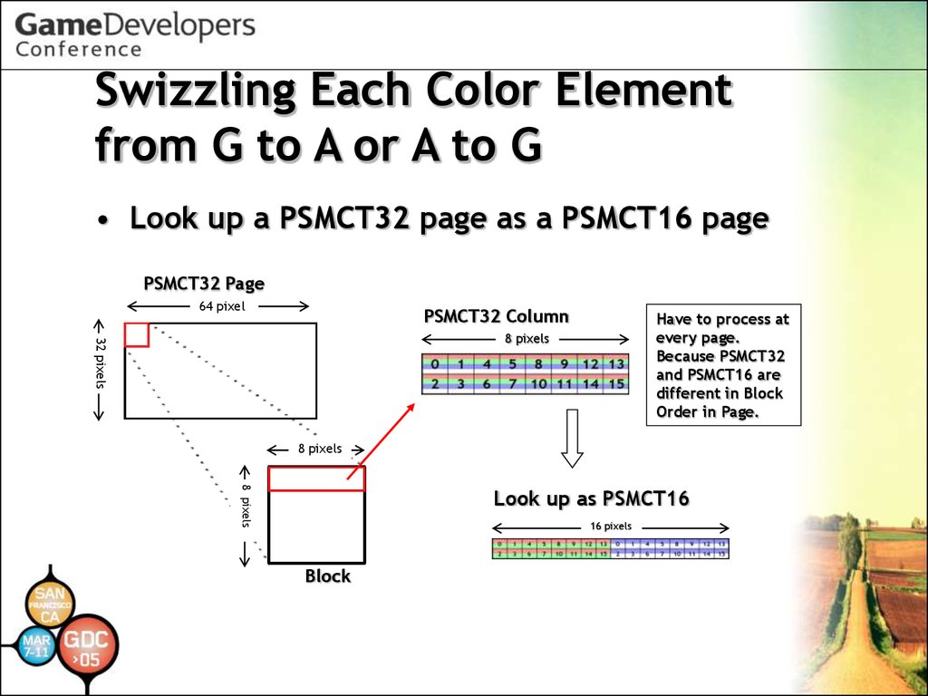
Swizzling Each Color Element
from G to A or A to G
• Look up a PSMCT32 page as a PSMCT16 page
PSMCT32 Page
64 pixel
PSMCT32 Column
Have to process at
every page.
Because PSMCT32
and PSMCT16 are
different in Block
Order in Page.
32 pixels
8 pixels
8 pixels
8 pixels
Look up as PSMCT16
16 pixels
Block

80.

Swizzling Each Color Element
from G to A or A to G
• Copy with FBMSK
Copy with FBMSK
0
1
4
5
8
9
12
13
0
1
4
5
8
9
12
13
2
3
6
7
10
11
14
15
2
3
6
7
10
11
14
15
Copy
Result PSMCT32
8 pixels
Mask Out
SCE_FRAME.FBMSK = 0x3FFF

81.

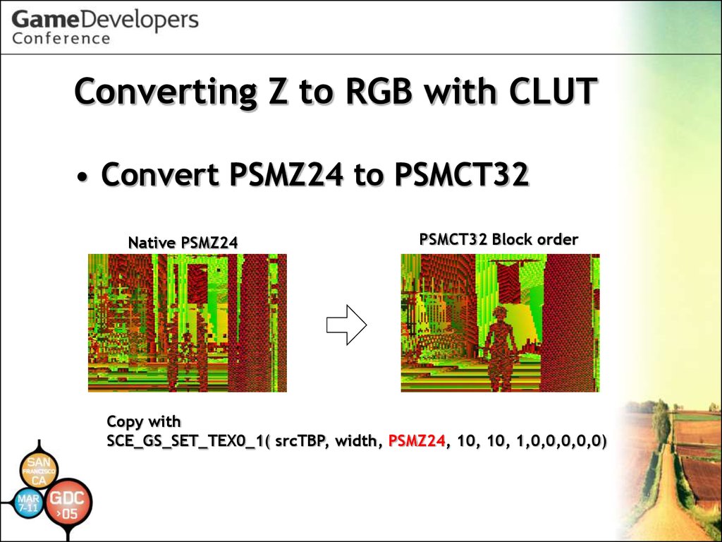
Converting Z to RGB with CLUT
• Convert PSMZ24 to PSMCT32
Native PSMZ24
PSMCT32 Block order
Copy with
SCE_GS_SET_TEX0_1( srcTBP, width, PSMZ24, 10, 10, 1,0,0,0,0,0)

82.

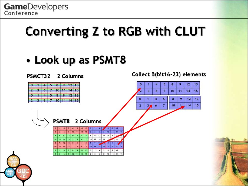
Converting Z to RGB with CLUT
• Look up as PSMT8
PSMCT32
2 Columns
PSMT8 2 Columns
Collect B(bit16-23) elements

83.

Converting Z to RGB with CLUT
• Requires many tiny sprites such as
8x2 or 4x2, so it's inefficient if
creating on VU
• When converting a larger area,
using Tile Base Processing for
sharing a packet is recommended

84.

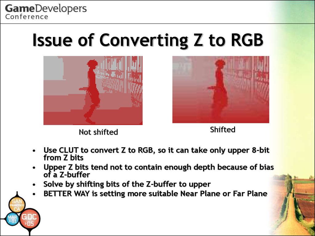
Issue of Converting Z to RGB
Not shifted
Shifted
• Use CLUT to convert Z to RGB, so it can take only upper 8-bit
from Z bits
• Upper Z bits tend not to contain enough depth because of bias
of a Z-buffer
• Solve by shifting bits of the Z-buffer to upper
• BETTER WAY is setting more suitable Near Plane or Far Plane

85.

Shifting Z bits toward Upper Side
Step1 Save G of the Z-buffer in alpha plane
Step2 Add B the same number of times as shift bits
to itself for biasing B
Step3 Put saved G into lower B with alpha blending
(protect upper B by FBMASK of FRAME
register)
※ 24-bit Z-buffer case
B:17-23 bit G:8-16 bit R:0-7 bit

86.

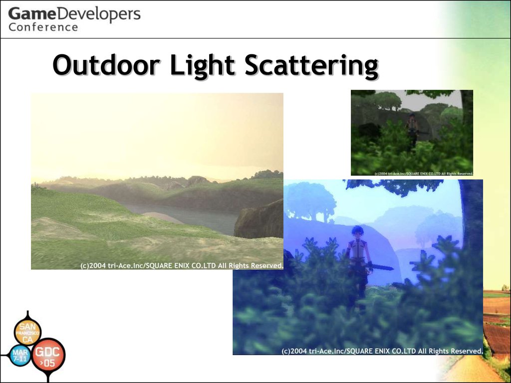
Outdoor Light Scattering

87.

Outdoor Light Scattering
• Implementation of:
– Naty Hoffman, Arcot J Preetham. "Rendering Outdoor
Light Scattering in Real Time“ GDC 2002.
• Glare Effects and DOF work good
enough on Reduced Frame Buffer,
but OLS requires higher resolution, so
OLS tends to need more pixel-fill costs
• Takes 13-39Hsync (typically), 57Hsync

88.

Outdoor Light Scattering
• Adopting Tile Base Processing
• High OLS fillrate causes a bottleneck, so computing
colors and making primitives are processed by VU1
during previous tile rendering
Create Tile0
Kick Tile0
Create Next Tile1

89.

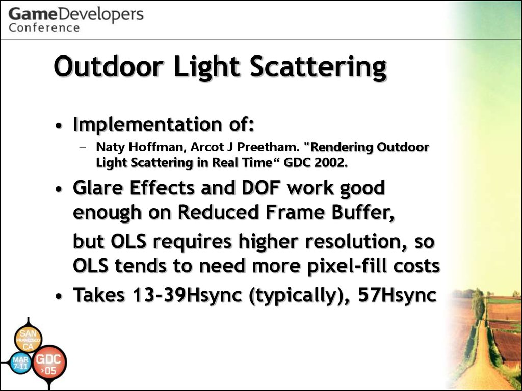
Additional Parameters
• 2nd Mie Coefficients
– Can represent more complex coloring
– No change to fill costs
Green color added by 2nd Mie

90.

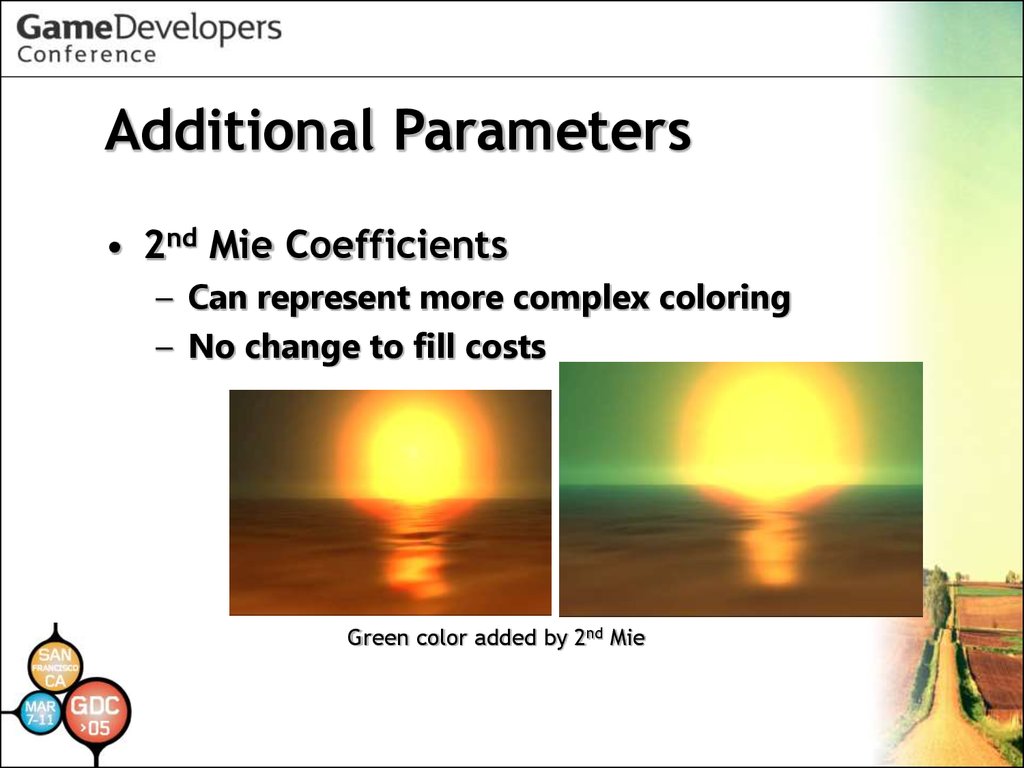
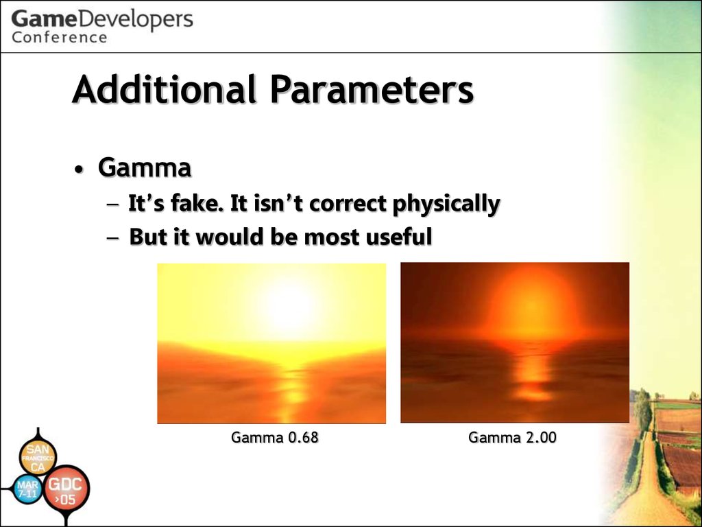
Additional Parameters
• Gamma
– It’s fake. It isn’t correct physically
– But it would be most useful
Gamma 0.68
Gamma 2.00

91.

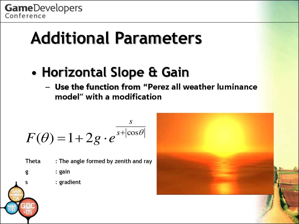
Additional Parameters
• Horizontal Slope & Gain
– Use the function from “Perez all weather luminance
model” with a modification
F ( ) 1 2 g e
s
s cos
Theta
: The angle formed by zenith and ray
g
: gain
s
: gradient

92.

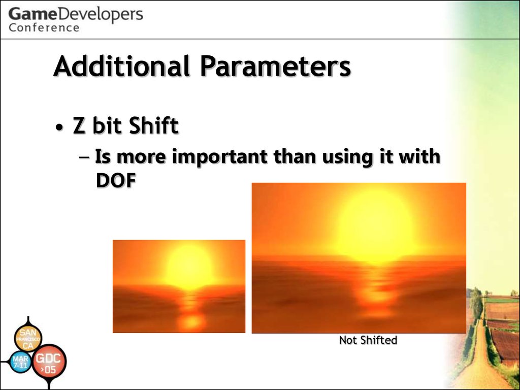
Additional Parameters
• Z bit Shift
– Is more important than using it with
DOF
Not Shifted

93.

OLS - Episode
• Shifting Z bits causes a side effect where objects in the
foreground tend to be colored by clamping values
• Artists found and started shifting Z bits as color
correction, so we provided inexpensive emulation of
coloring

94.

Spherical Harmonics Lighting

95.

How to use SH Lighting easily?
• Use DirectX9c!
– Of course, we know you want to
implement it yourselves
– But SH Lighting implementation on
DirectX9c is useful to understand it
– You should look over its
documentation and samples

96.

Reason to use SH Lighting on PS2
• Photo-realistic
lighting
Global Illumination
with Light Transport
Traditional Lighting with an
omni-directional light and
Volumetric Shadow

97.

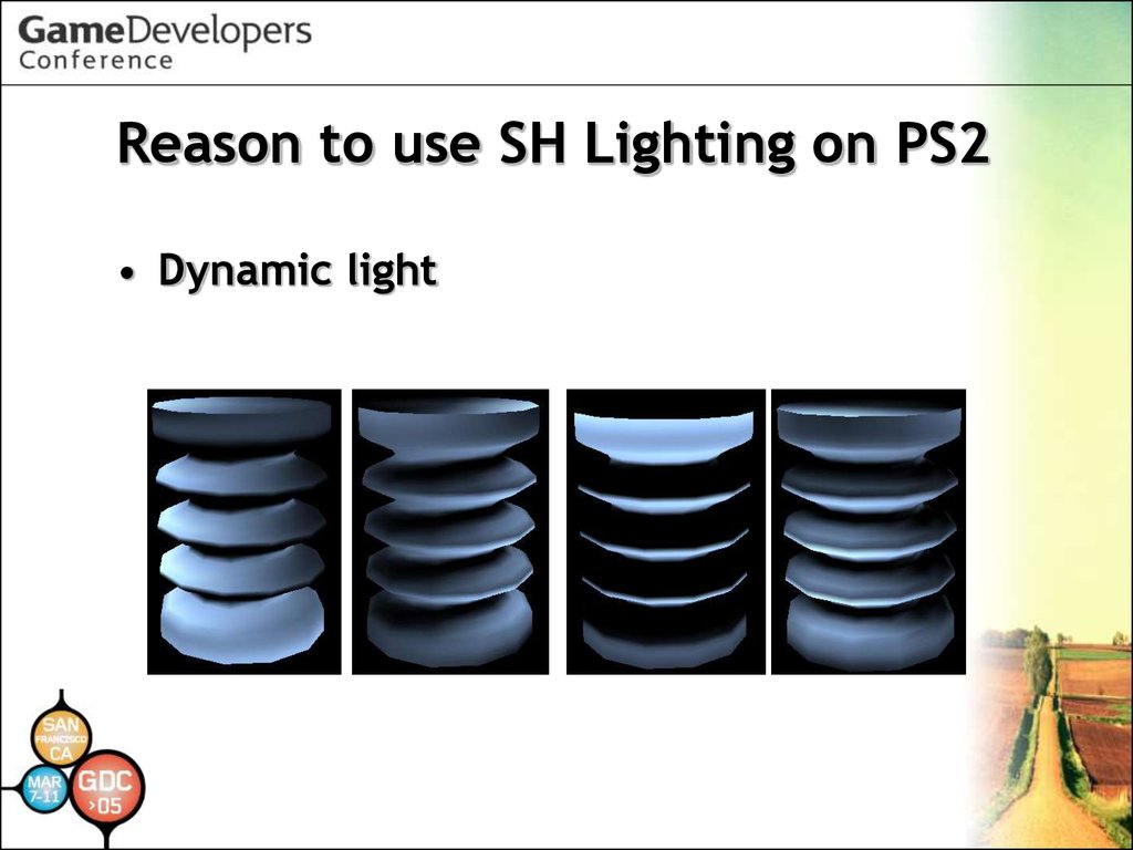
Reason to use SH Lighting on PS2
• Dynamic light

98.

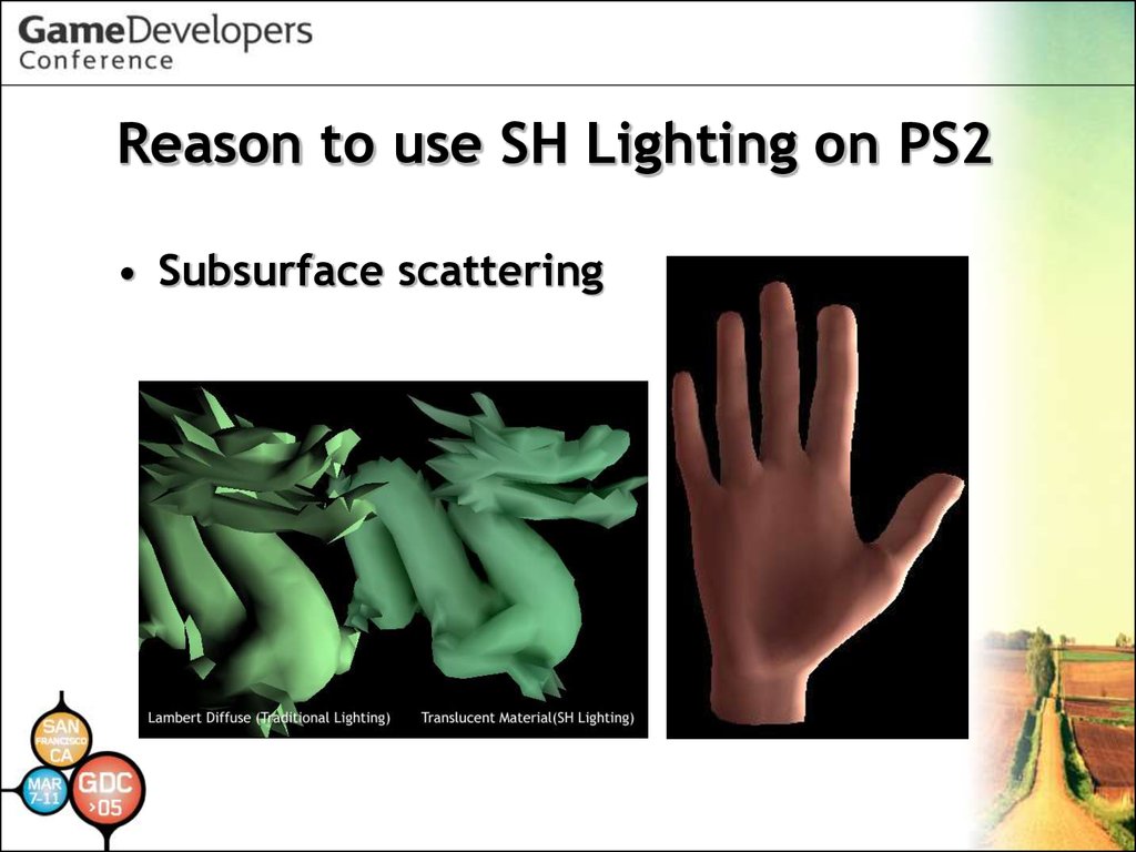
Reason to use SH Lighting on PS2
• Subsurface scattering

99.

PRT
• Precomputed Radiance Transfer
was published by Peter Pike Sloan
et al. in SIGRAPH 2002
– Compute incident light from all
directions off line and compress it
– Use compressed data for illuminating
surfaces in real-time

100.

What to do with PRT
• Limited real-time global
illumination
– Basically objects mustn't deform
– Basically objects mustn't move
• Limited B(SS)RDF simulation
– Lambertian Diffuse
– Glossy Specular
– Arbitrary (low frequency) BRDF

101.

Limited Animation
• SH Light position can move or rotate
– But SH lights are regarded as infinite
distance lights (directional light)
• SH Light color and intensity can be
animated
– IBL can be used
• Objects can move or rotate
– But if objects affect each other, those
objects can’t move
• Because light effects are pre-computed!

102.

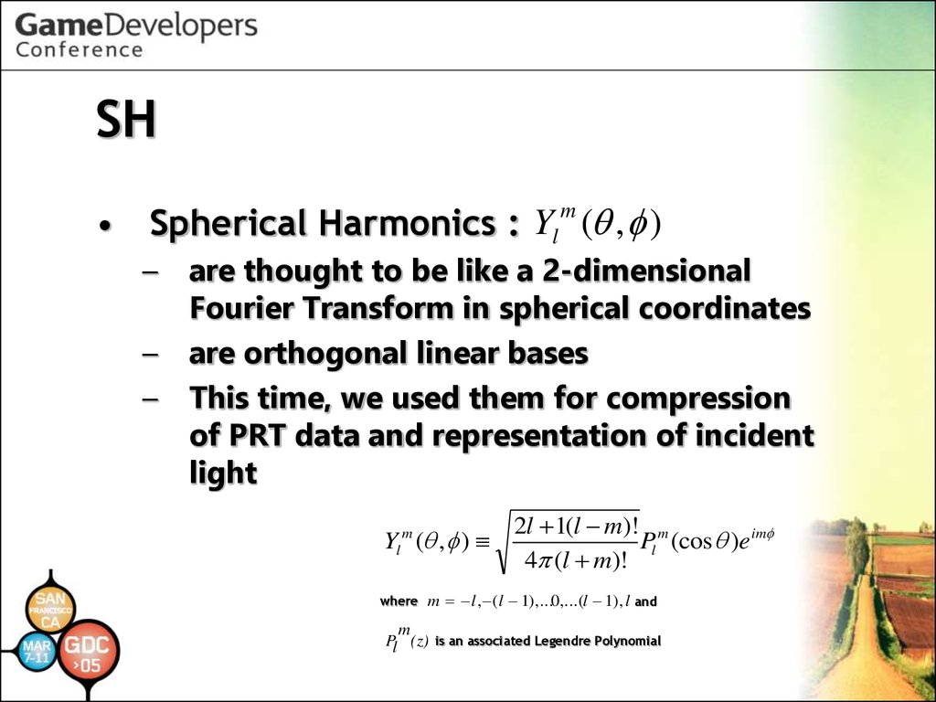
SH
• Spherical Harmonics : Yl ( , )
m
–
–
–
are thought to be like a 2-dimensional
Fourier Transform in spherical coordinates
are orthogonal linear bases
This time, we used them for compression
of PRT data and representation of incident
light
Yl m ( , )
where
2l 1(l m)! m
Pl (cos )eim
4 (l m)!
m l , ( l 1),...0,...(l 1), l and
m
Pl (z)
is an associated Legendre Polynomial

103.

How is data compressed?
• PRT data is considered as a response
to rays from all directions in 3Dspace
• Think of it as 2D-space, so as to
understand easily

104.

How is data compressed?
1
0.5
-1.5
-1
-0.5
0.5
1
1.5
-0.5
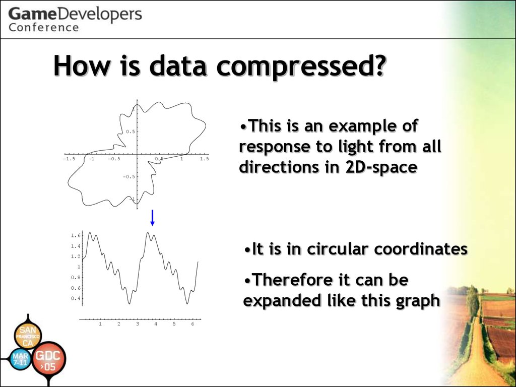
•This is an example of
response to light from all
directions in 2D-space
-1
1.6
•It is in circular coordinates
1.4
1.2
1
•Therefore it can be
expanded like this graph
0.8
0.6
0.4
1
2
3
4
5
6

105.

How is data compressed?
•This function can be
represented by the
Fourier series (set of
infinite trig functions)
1.6
1.4
1.2
1
0.8
0.6
0.4
1
2
3
4
5
6
• If there is a function like 2D Fourier
Transform in spherical coordinates; PRT
data can be compressed with it

106.

How is data compressed?
• You could think of Spherical
Harmonics as a 2D Fourier Transform
in spherical coordinates, so as to
understand easily

107.

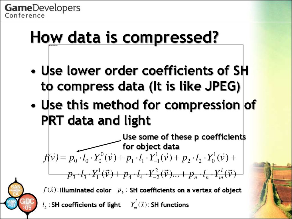
How data is compressed?
• Use lower order coefficients of SH
to compress data (It is like JPEG)
• Use this method for compression of
PRT data and light
Use some of these p coefficients
for object data
0
1
1
f(v ) p0 l0 Y0 (v ) p1 l1 Y 1 (v ) p2 l2 Y0 (v )
1
2
l
p3 l3 Y1 (v ) p4 l4 Y 2 (v )... pn ln Ym (v )
f ( x ) : Illuminated color
p k : SH coefficients on a vertex of object
l k : SH coefficients of light
l
Ym ( x ) : SH functions

108.

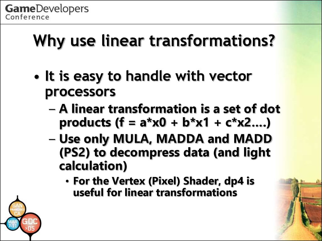
Why use linear transformations?
• It is easy to handle with vector
processors
– A linear transformation is a set of dot
products (f = a*x0 + b*x1 + c*x2….)
– Use only MULA, MADDA and MADD
(PS2) to decompress data (and light
calculation)
• For the Vertex (Pixel) Shader, dp4 is
useful for linear transformations

109.

Compare linear transformations
SH
Wavelet
PCA basis
Rotation
invariant
variant
variant
With few coef
soft (but
usable)
jaggy (depends
on a basis)
useless
(depends on
complexity)
High frequency
(specular)
useless (lots
of coef)
support
support
Specular
interreflection
possible
difficult
difficult
Handiness for
artists
easy
?
?
This comparison is based on current papers. Recent papers hardly
take up Spherical Harmonics, but we think it is still useful for game
engines

110.

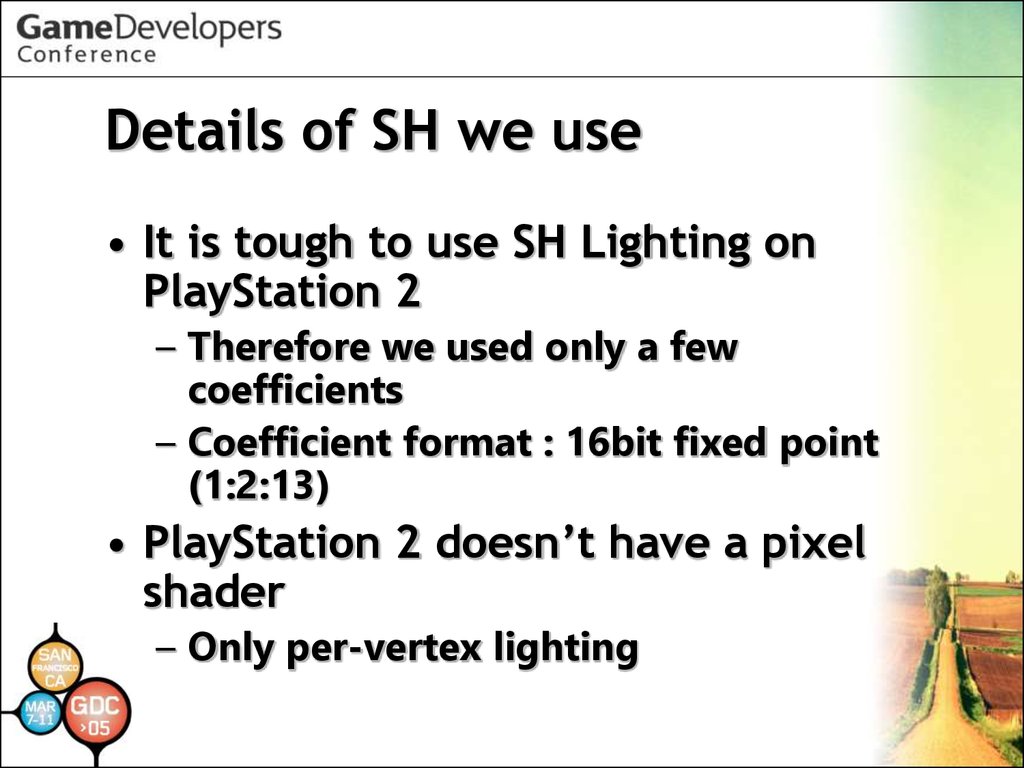
Details of SH we use
• It is tough to use SH Lighting on
PlayStation 2
– Therefore we used only a few
coefficients
– Coefficient format : 16bit fixed point
(1:2:13)
• PlayStation 2 doesn’t have a pixel
shader
– Only per-vertex lighting

111.

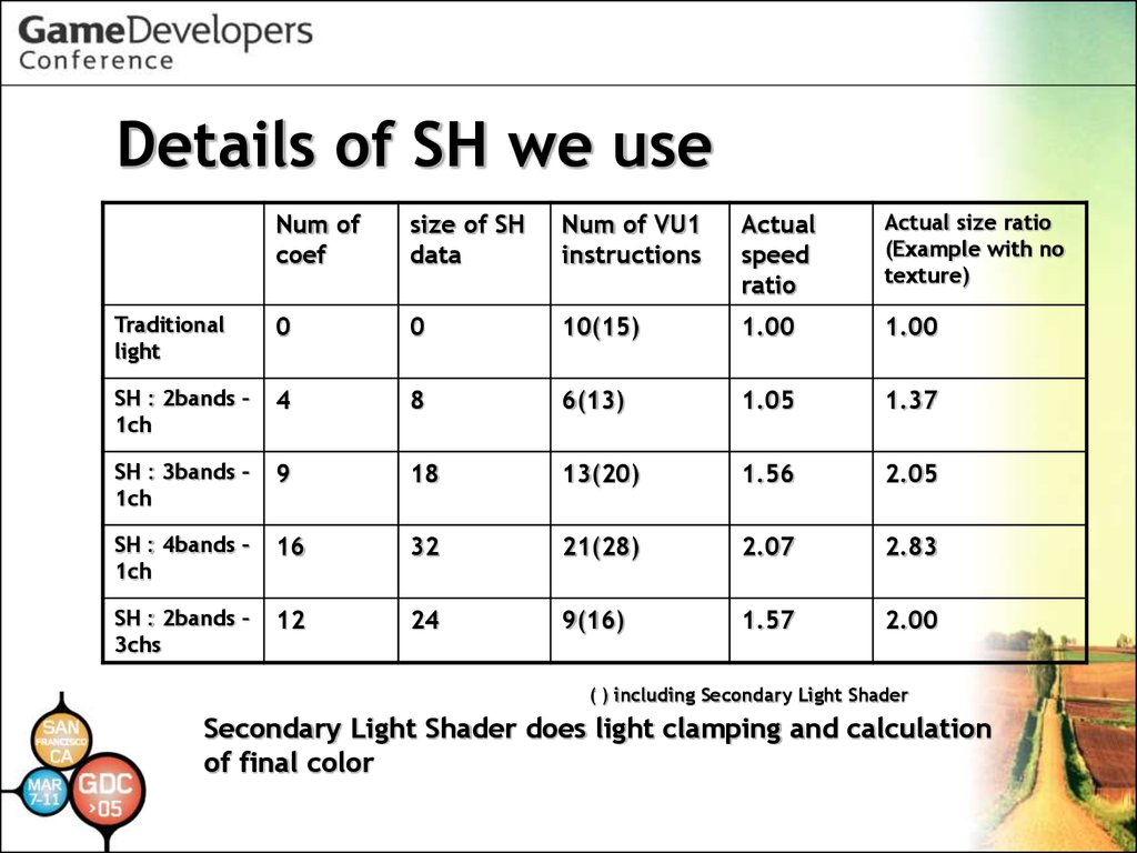
Details of SH we use
Num of
coef
size of SH
data
Num of VU1
instructions
Actual
speed
ratio
Actual size ratio
(Example with no
texture)
Traditional
light
0
0
10(15)
1.00
1.00
SH : 2bands –
1ch
4
8
6(13)
1.05
1.37
SH : 3bands –
1ch
9
18
13(20)
1.56
2.05
SH : 4bands –
1ch
16
32
21(28)
2.07
2.83
SH : 2bands –
3chs
12
24
9(16)
1.57
2.00
( ) including Secondary Light Shader
Secondary Light Shader does light clamping and calculation
of final color

112.

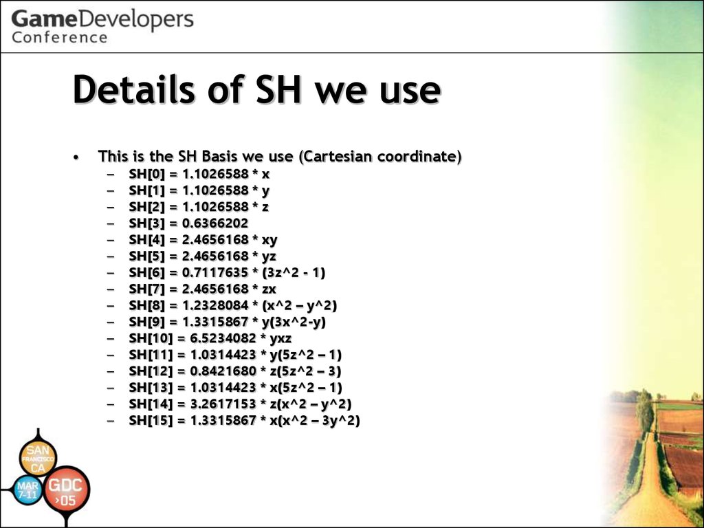
Details of SH we use
This is the SH Basis we use (Cartesian coordinate)
–
–
–
–
–
–
–
–
–
–
–
–
–
–
–
–
SH[0] = 1.1026588 * x
SH[1] = 1.1026588 * y
SH[2] = 1.1026588 * z
SH[3] = 0.6366202
SH[4] = 2.4656168 * xy
SH[5] = 2.4656168 * yz
SH[6] = 0.7117635 * (3z^2 - 1)
SH[7] = 2.4656168 * zx
SH[8] = 1.2328084 * (x^2 – y^2)
SH[9] = 1.3315867 * y(3x^2-y)
SH[10] = 6.5234082 * yxz
SH[11] = 1.0314423 * y(5z^2 – 1)
SH[12] = 0.8421680 * z(5z^2 – 3)
SH[13] = 1.0314423 * x(5z^2 – 1)
SH[14] = 3.2617153 * z(x^2 – y^2)
SH[15] = 1.3315867 * x(x^2 – 3y^2)

113.

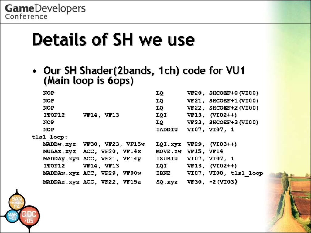
Details of SH we use
• Our SH Shader(2bands, 1ch) code for VU1
(Main loop is 6ops)
NOP
NOP
NOP
ITOF12
NOP
NOP
tls1_loop:
MADDw.xyz
MULAx.xyz
MADDAy.xyz
ITOF12
MADDAw.xyz
MADDAz.xyz
VF14, VF13
VF30, VF23, VF15w
ACC, VF20, VF14x
ACC, VF21, VF14y
VF14, VF13
ACC, VF29, VF00w
ACC, VF22, VF15z
LQ
LQ
LQ
LQI
LQ
IADDIU
VF20,
VF21,
VF22,
VF13,
VF23,
VI07,
SHCOEF+0(VI00)
SHCOEF+1(VI00)
SHCOEF+2(VI00)
(VI02++)
SHCOEF+3(VI00)
VI07, 1
LQI.xyz
MOVE.zw
ISUBIU
LQI
IBNE
SQ.xyz
VF29,
VF15,
VI07,
VF13,
VI07,
VF30,
(VI03++)
VF14
VI07, 1
(VI02++)
VI00, tls1_loop
-2(VI03)

114.

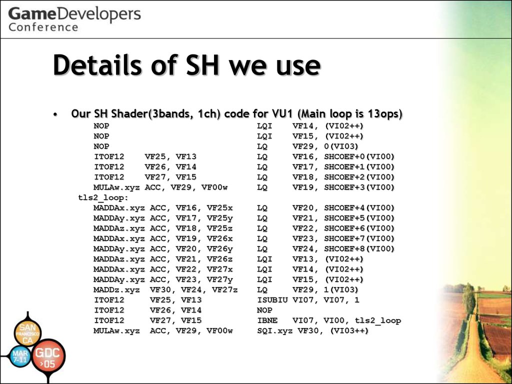
Details of SH we use
Our SH Shader(3bands, 1ch) code for VU1 (Main loop is 13ops)
NOP
NOP
NOP
ITOF12
VF25, VF13
ITOF12
VF26, VF14
ITOF12
VF27, VF15
MULAw.xyz ACC, VF29, VF00w
tls2_loop:
MADDAx.xyz ACC, VF16, VF25x
MADDAy.xyz ACC, VF17, VF25y
MADDAz.xyz ACC, VF18, VF25z
MADDAx.xyz ACC, VF19, VF26x
MADDAy.xyz ACC, VF20, VF26y
MADDAz.xyz ACC, VF21, VF26z
MADDAx.xyz ACC, VF22, VF27x
MADDAy.xyz ACC, VF23, VF27y
MADDz.xyz VF30, VF24, VF27z
ITOF12
VF25, VF13
ITOF12
VF26, VF14
ITOF12
VF27, VF15
MULAw.xyz ACC, VF29, VF00w
LQI
LQI
LQ
LQ
LQ
LQ
LQ
VF14,
VF15,
VF29,
VF16,
VF17,
VF18,
VF19,
(VI02++)
(VI02++)
0(VI03)
SHCOEF+0(VI00)
SHCOEF+1(VI00)
SHCOEF+2(VI00)
SHCOEF+3(VI00)
LQ
VF20, SHCOEF+4(VI00)
LQ
VF21, SHCOEF+5(VI00)
LQ
VF22, SHCOEF+6(VI00)
LQ
VF23, SHCOEF+7(VI00)
LQ
VF24, SHCOEF+8(VI00)
LQI
VF13, (VI02++)
LQI
VF14, (VI02++)
LQI
VF15, (VI02++)
LQ
VF29, 1(VI03)
ISUBIU VI07, VI07, 1
NOP
IBNE
VI07, VI00, tls2_loop
SQI.xyz VF30, (VI03++)

115.

Details of SH we use
• Engineers think that SH can be
used with at least the 5th order (25
coefficients for each channel)
• Practically, artists think SH is
useful with even the 2nd order (4
coefficients)
• Artists will think about how to use
it efficiently

116.

Differences in appearance
• The 2nd order is inaccurate
– However, it’s useful (soft shading)
• The 3rd and 4th are similar
– The 3rd is useful considering costs

117.

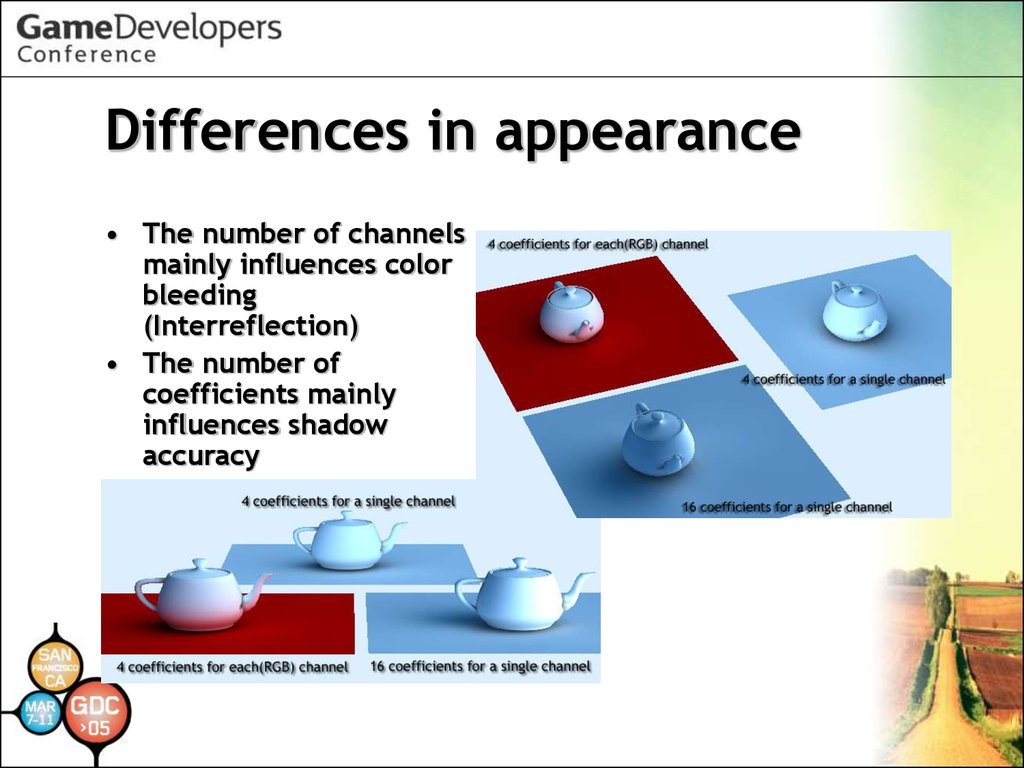
Differences in appearance
• The number of channels
mainly influences color
bleeding
(Interreflection)
• The number of
coefficients mainly
influences shadow
accuracy

118.

Differences in appearance
• For sub-surface scattering,
color channels tend to be
more important than the
number of coefficients

119.

Harmonize SH traditionally
• We harmonize SH
Lighting with
traditional lights:
– There is a function by
which hemisphere light
coefficients come from
linear coefficients of
Spherical Harmonics
– For Phong (Specular)
lighting, we process
diffuse and ambient
with SH Shader, and
process specular with
traditional lighting

120.

Side effects of SH Lighting
• Useful
– SH Lighting (Shading)
is smoother than
traditional lighting
– Especially, it is useful
for low-poly-count
models
– It works as a low pass
filter

121.

Side effects of SH Lighting
• Disadvantage
– SH is an
approximation of
BRDF
– But using only a few
coefficients causes
incorrect
approximation
Green : Approx.
Blue : Actual
This point is darker
than actual
This point is brighter
than actual
Actual

122.

Our precomputation engine
• supports :
–
–
–
–
–
Lambert diffuse shading
Soft-edged shadow
Sub-surface scattering
Diffuse interreflection
Light transport (detail later)

123.

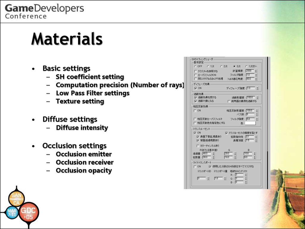
Materials
• Basic settings
–
–
–
–
SH coefficient setting
Computation precision (Number of rays)
Low Pass Filter settings
Texture setting
• Diffuse settings
– Diffuse intensity
• Occlusion settings
– Occlusion emitter
– Occlusion receiver
– Occlusion opacity

124.

Materials
• Interreflection settings
–
–
–
–
Interreflection intensity
Number of passes
Interreflection low pass filter
Color settings
• Translucent settings
–
–
–
–
–
–
Enabling single scattering
Enabling multi scattering
Diffusion directivity
Surface thickness
Permeability
Diffusion amount
• Light Transport settings

125.

Algorithms for PRT
• Based on (Stratified) Monte Carlo
ray-tracing

126.

PRT Engine [1st stage]
• Calculate diffuse and occlusion
coefficients by Monte Carlo raytracing:
– Cast rays for all hemispherical
directions
– Then integrate diffuse BRDF with the
SH basis and calculate occlusion SH
coefficients (occluded = 1.0, passed =
0.0)

127.

PRT Engine [2nd stage]
• Calculate sub-surface scattering
coefficients with diffuse
coefficients by ray-tracing
– We used modified Jensen’s model
(using 2 omni-directional lights) for
simulating sub-surface scattering

128.

PRT Engine [3rd stage]
• Calculate interreflection
coefficients from diffuse and subsurface scattering coefficients:
– Same as computing diffuse BRDF
coefficients
– Cast rays for other surfaces and
integrate their SH coefficients with
diffuse BRDF

129.

PRT Engine [4th stage]
• Repeat from the 2nd stage for
number of passes
• After that, Final Gathering (gather
all coefficients and apply a low
pass filter)

130.

Optimize precomputation
• To optimize finding of rays and
polygon intersection, we used
those typical approaches (nothing
special)
– Multi-threading
– Using SSE2 instructions
– Cache-caring data

131.

Optimize precomputation
• Multi-threading for every calculation
was very efficient
– Example result (with dual Pentium Xeon 3.0GHz)
Number
1
of threads
2
3
4
5
Speed
ratio
1.8
2.0
2.2
2.1
1.0

132.

Optimize precomputation
• SSE2 (inline assembler) for finding
intersections was quite efficient
– Example result (with dual Pentium Xeon 3.0GHz)
Speed
ratio
No SSE2
SSE2 for
tree
traversal
SSE2 for ray- Both
polygon
intersection
1.0
5.0
2.4
12.0

133.

Optimize precomputation
• File Caching System
– SH coefficients and object geometry
are cached in files for each object
– Use cache files unless parameters are
changed

134.

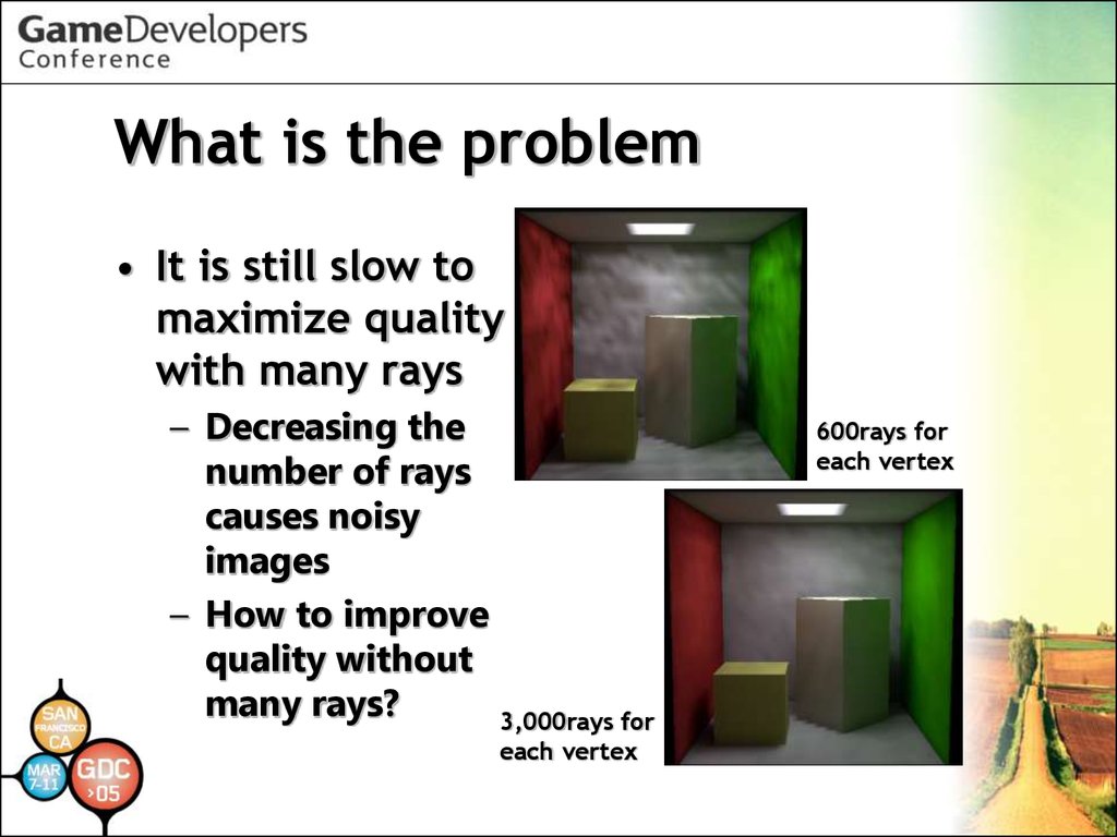
What is the problem
• It is still slow to
maximize quality
with many rays
– Decreasing the
number of rays
causes noisy
images
– How to improve
quality without
many rays?
3,000rays for
each vertex
600rays for
each vertex

135.

Solving the problem
• We used 2-stage low pass filters to
solve it
– Diffuse interreflection low pass filter
– Final low pass filter

136.

Solving the problem
• We used Gaussian Filter for a low pass
filter
– Final LPF was efficient to reduce noise
– But it caused inaccurate result
• Therefore we used a pre-filter for
diffuse interreflection
– Diffuse interreflection LPF works as
irradiance caching
– Diffuse interreflection usually causes noisy
images
– Reducing diffuse interreflection noise is
efficient

137.

Solving the problem
• Using too strong LPF causes inaccurate
images
– Be careful using LPF
3,000rays without LPF
600rays with LPF
(61seconds)
(22seconds)

138.

Light Transport
• It is our little technique for expanding
SH Lighting Shader
– It is feasible to represent all frequency
lighting (not specular) and area lights
– BUT! Light position can't be animated
– Only light color and intensity can be
animated
– Some lights don’t move
• For example, torch in a dungeon, lights in a house
• Particularly, most light sources in the background
don’t need to move

139.

Details of Light Transport
• It is not used on the Spherical
Harmonic basis
– Spherical Harmonics are orthogonal
– It means that the coefficients are
independent of each other
– You can use some of (SH) coefficients
for other coefficients on a different
basis

140.

Details of Light Transport
• To obtain Light Transport coefficients, the
precomputation engine calculates all their
incoming coefficients from other surfaces
– It means that Light Transport coefficients have the
same Light Transport energy that the surfaces collect
from other surfaces
– And surfaces which emit light give energy to other
surfaces
• Without modification to existing SH Lighting
Shader, it multiplies Light Transport
coefficients by light color and intensity
– They are just like vertex color multiplied by specific
intensity and color

141.

Details of Light Transport
• They are automatically computed
by existing global illumination
engine
– When you set energy parameters into
some coefficients, a precomputation
engine for diffuse interreflection will
transmit them to other surfaces

142.

Result of Light Transport
Light Transport
•11.29Hsync 6,600vertices
•9,207,000vertices/sec
Spherical Harmonics
(4 coefficients for each channel)
•15.32Hsync 7,488vertices
•7,698,000vertices/sec

143.

Image Based Lighting
• Our SH Lighting engine supports
Image Based Lighting
– It is too expensive to compute light
coefficients in every frame for PlayStation 2
– Therefore light coefficients are
precomputed off line
– IBL lights can be animated with color,
intensity, rotation, and linear interpolation
between different IBL lights

144.

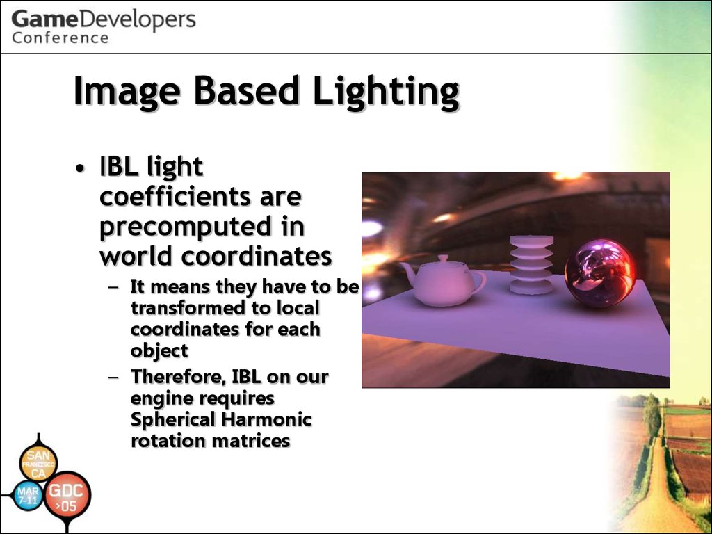
Image Based Lighting
• IBL light
coefficients are
precomputed in
world coordinates
– It means they have to be
transformed to local
coordinates for each
object
– Therefore, IBL on our
engine requires
Spherical Harmonic
rotation matrices

145.

SH rotation
• To obtain Spherical Harmonic
rotation matrices is one of the
problems of handling Spherical
Harmonics
– We used "Evaluation of the rotation
matrices in the basis of real spherical
harmonics"
– It was easy to implement

146.

SH animation
• Our SH Lighting engine supports
limited animation
– Skinning
– Morphing

147.

SH skinning
• Skinning is only for the
1st and 2nd order
coefficients
– They are just linear
– Therefore, you can use
regular rotation matrices
for skinning
– If you want to rotate
above the 2nd order
coefficients (they are nonlinear), you have to use SH
rotation matrices
– But it is just rotation
– Shadow, interreflection
and sub-surface scattering
are incorrect

148.

SH morphing
• Morphing is linear
interpolation
between different
Spherical Harmonic
coefficients
– It is just linear
interpolation, so
transitional values are
incorrect
– But it supports all types
of SH coefficients
(including Light
Transport)

149.

Future work
• Using high precision buffer and pixel
shader!!
• More precise Glare Effects in optics
• Natural Blur function not Gaussian
• Diaphragm-shaped Blur
• Seamless and Hopping-free DOF along
depth direction
• OLS using HDR values
• Higher quality slight blur effect

150.

Future Work
• Distributed precomputation engine
• SH Lighting for next-gen hardware
– Try: Thomas Annen et al. EGSR 2004
“Spherical Harmonic Gradients for MidRange Illumination”
– More generality for using SH lighting
– IBL map
• Try other methods for real-time
global illumination

151.

References
• Masaki Kawase. "Frame Buffer Postprocessing Effects in
DOUBLE-S.T.E.A.L (Wreckless)“ GDC 2003.
• Masaki Kawase. "Practical Implementation of High Dynamic
Range Rendering“ GDC 2004.
• Naty Hoffman et al. "Rendering Outdoor Light Scattering in
Real Time“ GDC 2002.
• Akio Ooba. “GS Programming Men-keisan: Cho SIMD Keisanho”
CEDEC 2002.
• Arcot J. Preetham. "Modeling Skylight and Aerial Perspective"
in "Light and Color in the Outdoors" SIGGRAPH 2003 Course.

152.

References
• Peter-Pike Sloan et al. “Precomputed Radiance Transfer for
Real-Time Rendering in Dynamic, Low-Frequency Lighting
Environments.” SIGGRAPH 2002.
• Robin Green. “Spherical Harmonic Lighting: The Gritty Details.
“ GDC 2003.
• Miguel A. Blanco et al. “Evaluation of the rotation matrices in
the basis of real spherical harmonics.” ECCC-3 1997.
• Henrik Wann Jensen “Realistic Image Synthesis Using Photon
Mapping.” A K PETERS LTD, 2001.
• Paul Debevec “Light Probe Image Gallery”
http://www.debevec.org/

153.

Acknowledgements
• We would like to thank
– Satoshi Ishii, Daisuke Sugiura for suggestion
to this session
– All other staff in our company for screen
shots in this presentation
– Mike Hood for checking this presentation
– Shinya Nishina for helping translation
– The Stanford 3D Scanning Repository
http://graphics.stanford.edu/data/3Dscanrep/

154.

Thank you for your attention.
• This slide presentation is available
on http://research.tri-ace.com/