Image warping / morphing

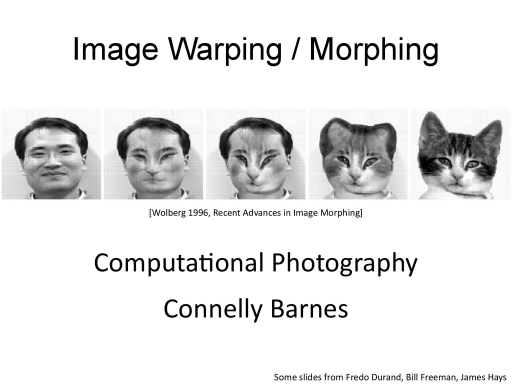
1. Image Warping / Morphing

[Wolberg 1996, Recent Advances in Image Morphing]
Computational Photography
Connelly Barnes
Some slides from Fredo Durand, Bill Freeman, James Hays

2. Morphing Video: Women in Art

• http://www.vimeo.com/1456037

3. Terminator 2 Morphing (1991)

Terminator 2 Clip (YouTube)

4. Image Warping in Biology

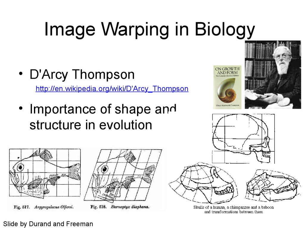
• D'Arcy Thompson
http://en.wikipedia.org/wiki/D'Arcy_Thompson
• Importance of shape and
structure in evolution
Slide by Durand and Freeman

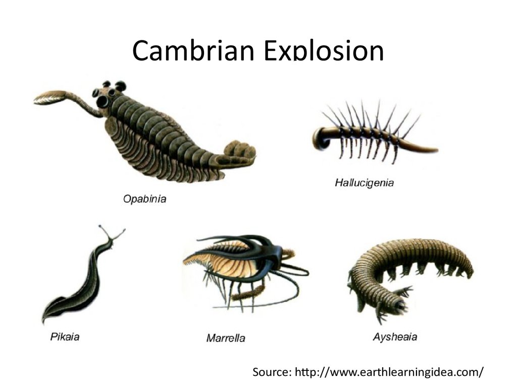
5. Cambrian Explosion

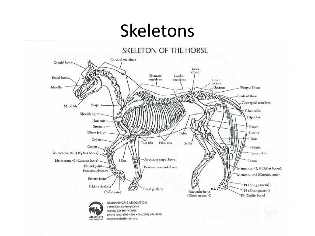
Source: http://www.earthlearningidea.com/

6. Skeletons

7. Skeletons

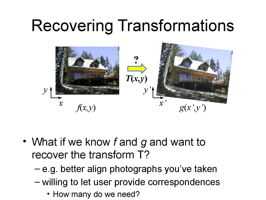
8. Recovering Transformations

?
T(x,y)
y’
y
x
f(x,y)
x’
g(x’,y’)
• What if we know f and g and want to
recover the transform T?
– e.g. better align photographs you’ve taken
– willing to let user provide correspondences
• How many do we need?

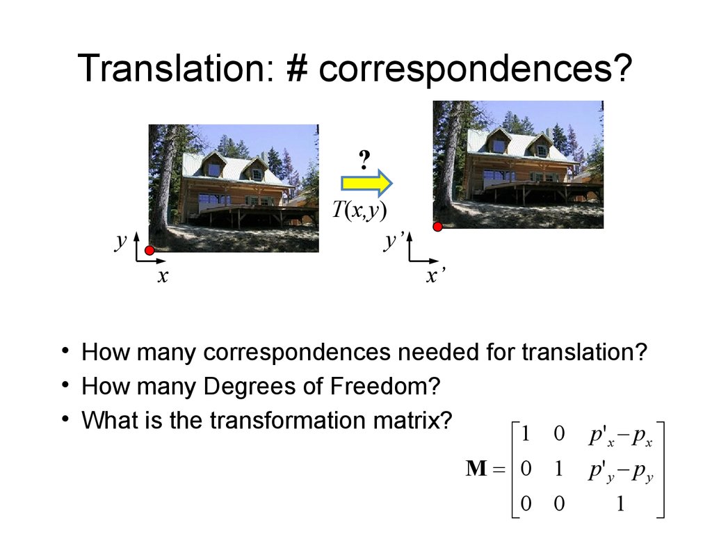
9. Translation: # correspondences?

?
T(x,y)
y’
y
x
x’
• How many correspondences needed for translation?
• How many Degrees of Freedom?
• What is the transformation matrix?
1 0 p' x p x
M 0 1 p' y p y
0 0
1

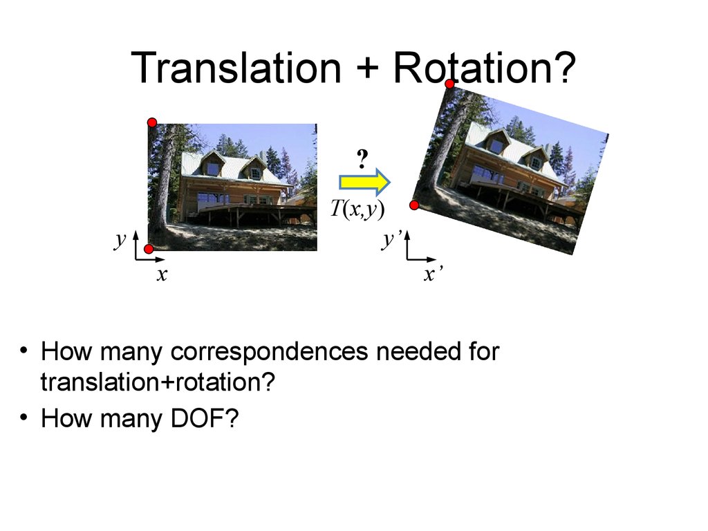
10. Translation + Rotation?

?
T(x,y)
y’
y
x
x’
• How many correspondences needed for
translation+rotation?
• How many DOF?

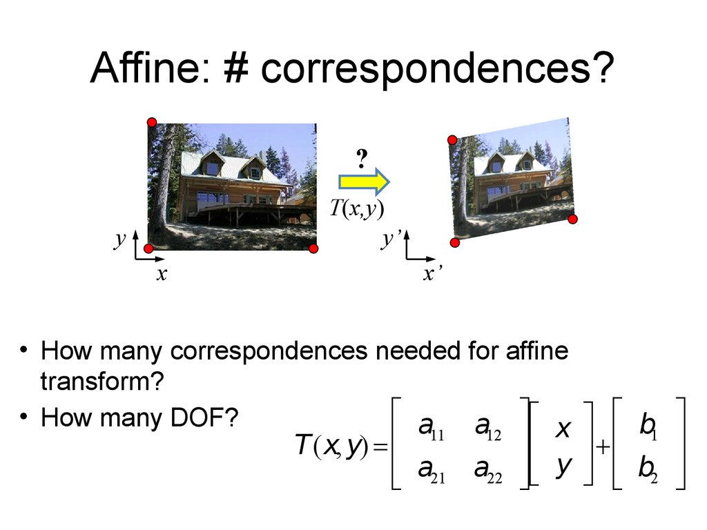
11. Affine: # correspondences?

?
T(x,y)
y’
y
x
x’
• How many correspondences needed for affine
transform?
a a
b
• How many DOF?
x
11
12
1
T(x, y)
a21 a22
+
y b2

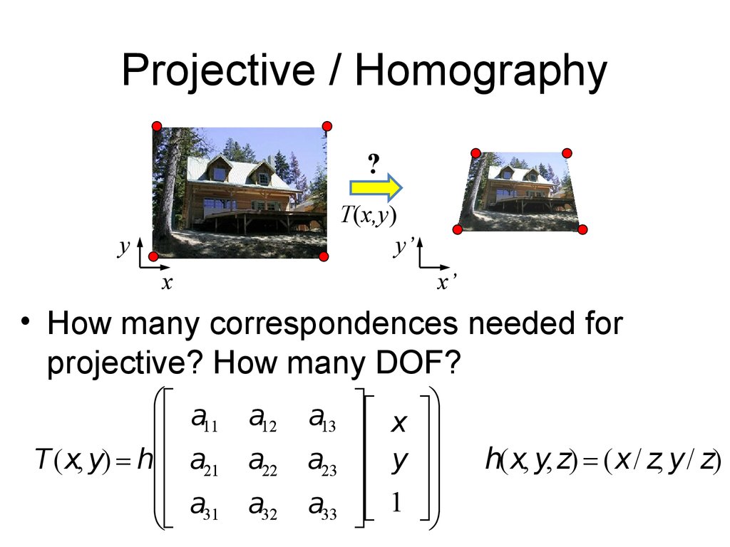
12. Projective / Homography

?
T(x,y)
y’
y
x
x’
• How many correspondences needed for
projective? How many DOF?
æ a a
ç 11 12
T(x, y) hç a21 a22
ç
ç a31 a32
è
a13 x ö÷
a23 y ÷
÷
a33 1 ÷
ø
h(x, y, z) (x/ z, y/ z)

13. Image Warping

T(x,y)
y’
y
x
f(x,y)
x’
g(x’,y’)
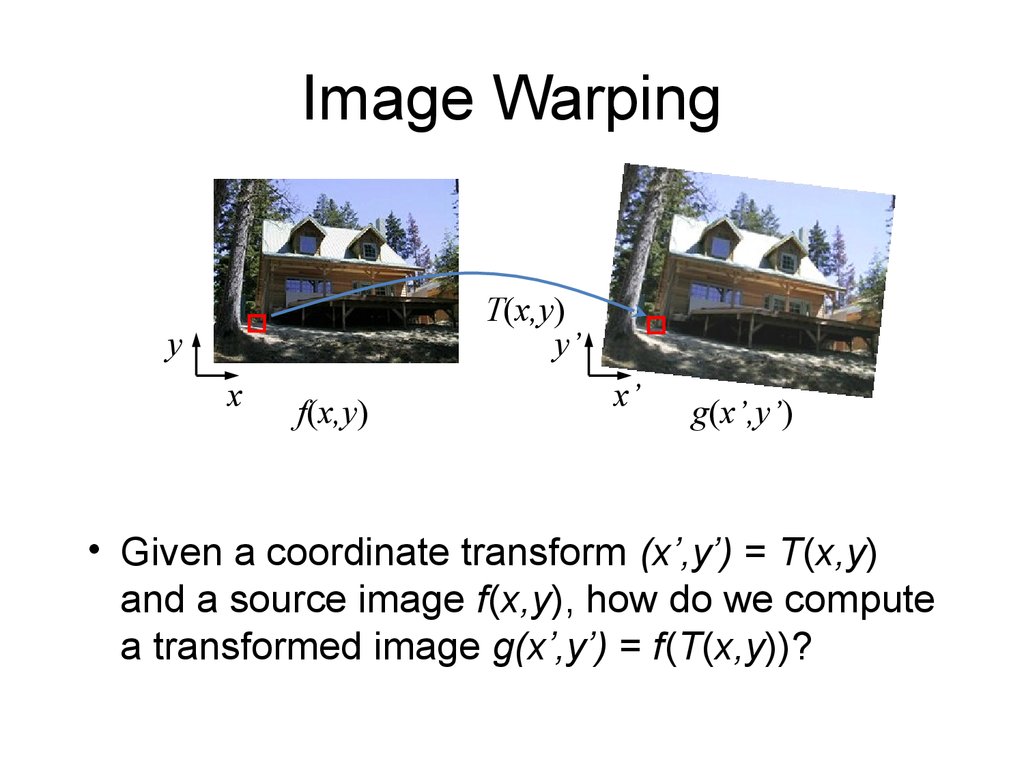
• Given a coordinate transform (x’,y’) = T(x,y)
and a source image f(x,y), how do we compute
a transformed image g(x’,y’) = f(T(x,y))?

14. Forward warping

T(x,y)
y’
y
x
(x,y)
x’
(x’,y’)
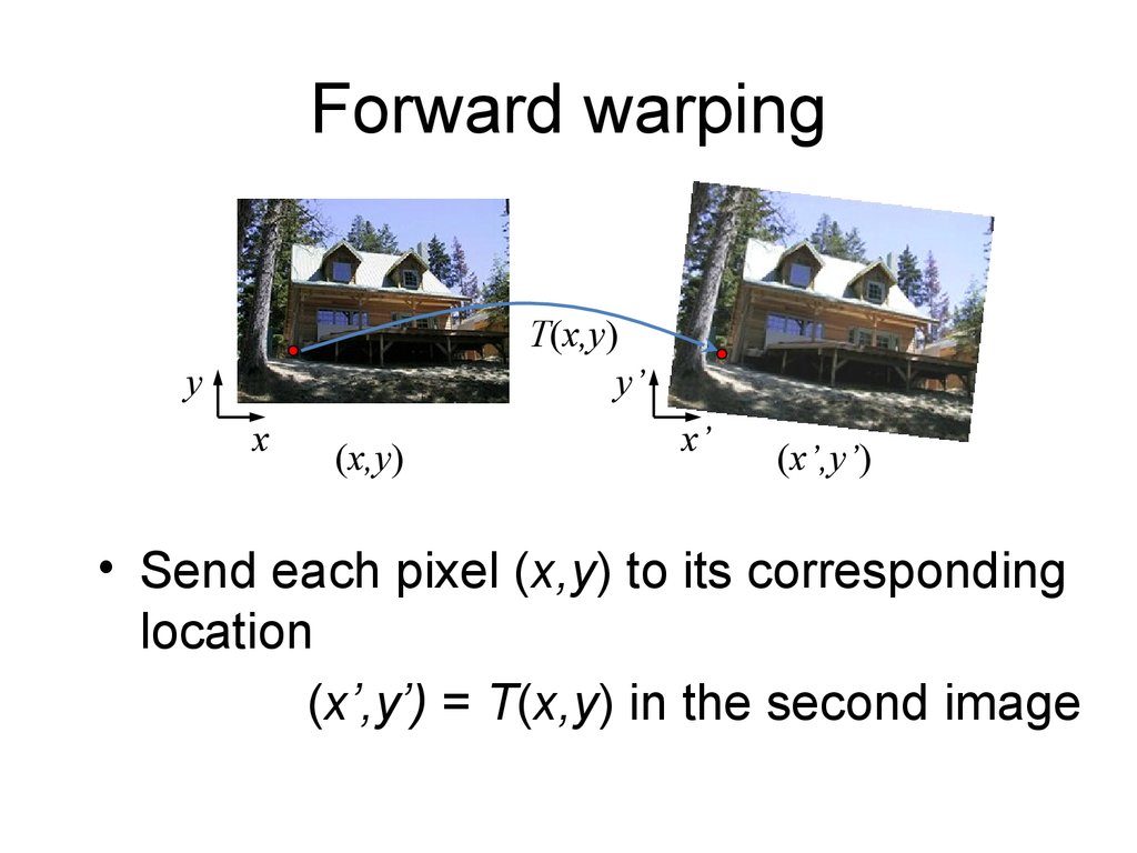
• Send each pixel (x,y) to its corresponding
location
(x’,y’) = T(x,y) in the second image

15. Forward warping

T(x,y)
y’
y
x
f(x,y)
x’
g(x’,y’)
Q: what if pixel lands “between” two pixels?
A: distribute color among neighboring pixels (x’,y’)
– Known as “splatting”
– Can also interpolate points in target image:
griddata (Matlab), scipy.interpolate.griddata (Python)

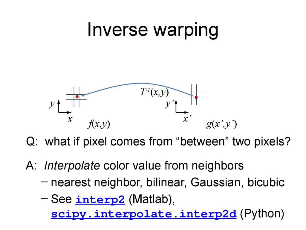
16. Inverse warping

T-1(x,y)
y’
y
x
(x,y)
x’
(x’,y’)
• Get each pixel color g(x’,y’) from its
corresponding location
(x,y) = T-1(x’,y’) in the first image

17. Inverse warping

T-1(x,y)
y’
y
x
f(x,y)
x’
g(x’,y’)
Q: what if pixel comes from “between” two pixels?
A: Interpolate color value from neighbors
– nearest neighbor, bilinear, Gaussian, bicubic
– See interp2 (Matlab),
scipy.interpolate.interp2d (Python)

18. Forward vs. inverse warping

• Q: Which is better?

19. Forward vs. inverse warping

• Q: Which is better?
• A: Usually inverse – eliminates holes
– However, it requires an invertible warp function
– Not always possible

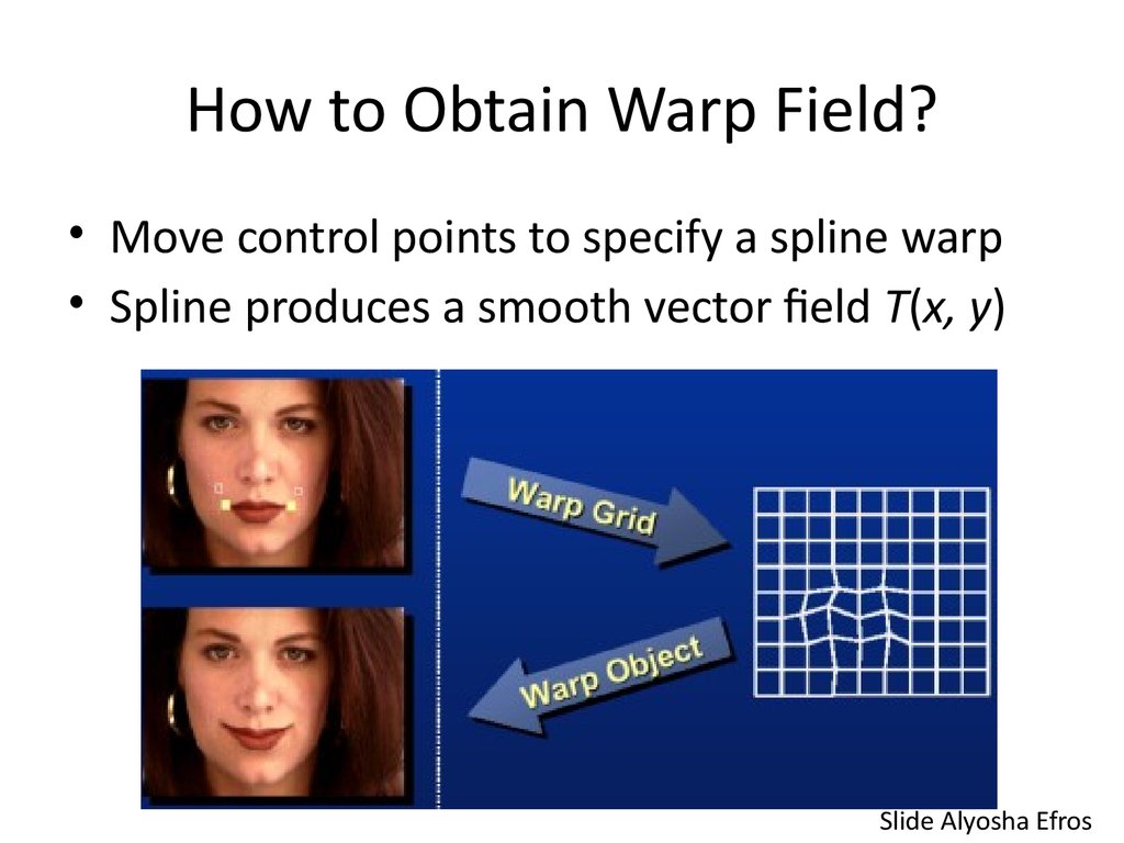
20. How to Obtain Warp Field?

• Move control points to specify a spline warp
• Spline produces a smooth vector field T(x, y)
Slide Alyosha Efros

21. Warp as Interpolation

• We are looking for a warping field
– A function that given a 2D point,
returns a warped 2D point
• We have a sparse number of correspondences
– These specify values of the warping field
• This is an interpolation problem
– Given sparse data, find smooth function

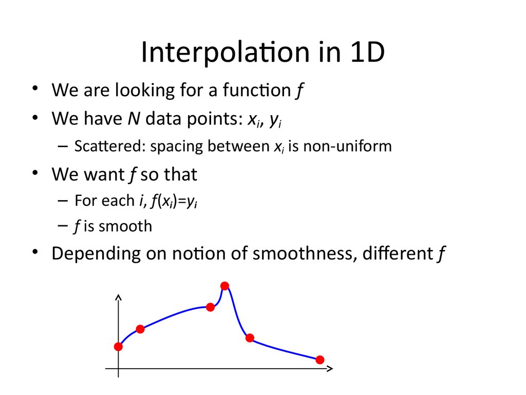
22. Interpolation in 1D

• We are looking for a function f
• We have N data points: xi, yi
– Scattered: spacing between xi is non-uniform
• We want f so that
– For each i, f(xi)=yi
– f is smooth
• Depending on notion of smoothness, different f

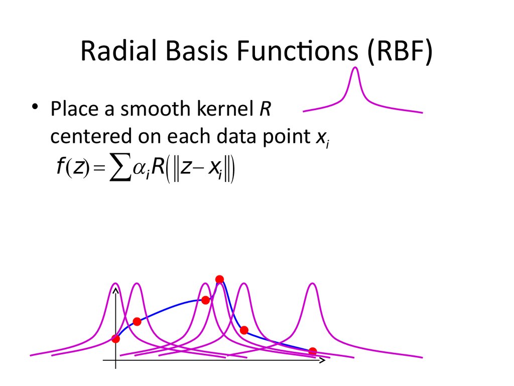
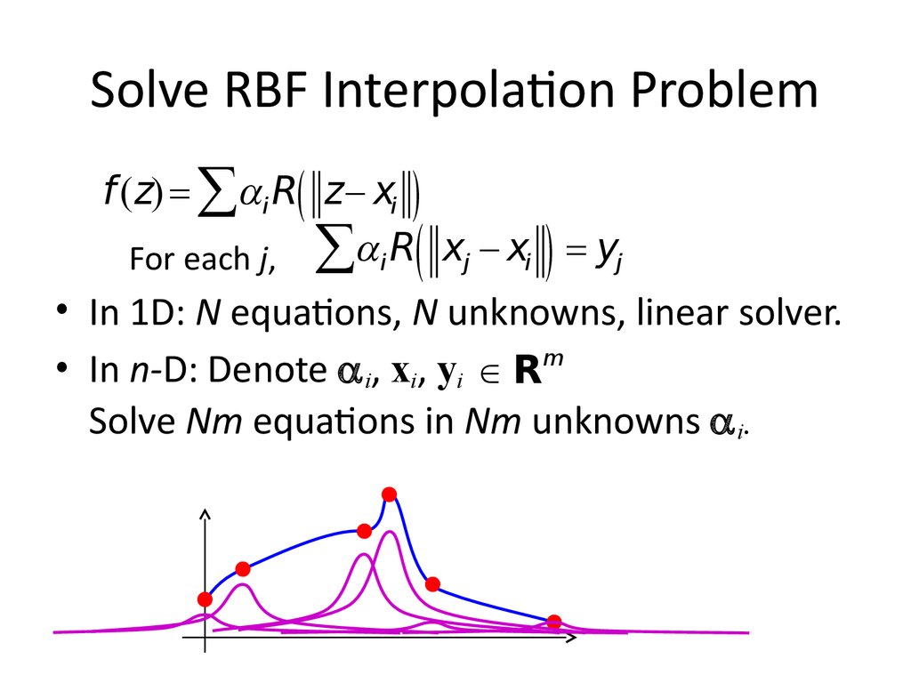
23. Radial Basis Functions (RBF)

• Place a smooth kernel R
centered on each data point xi
f (z) åai R( z xi )

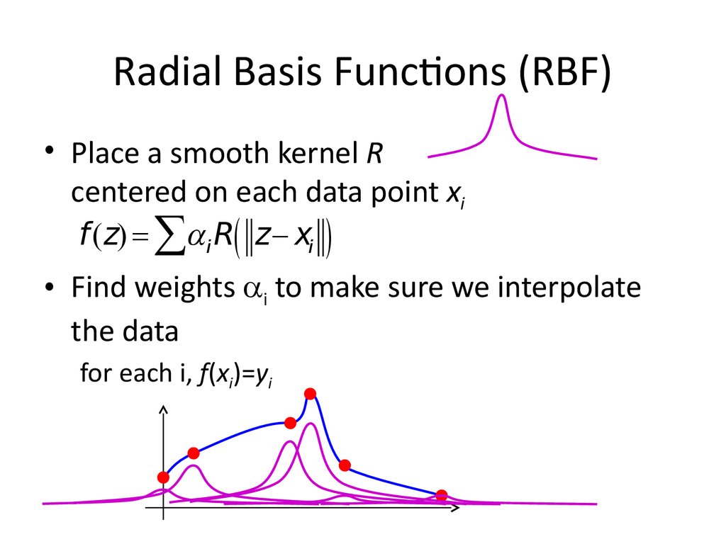
24. Radial Basis Functions (RBF)

• Place a smooth kernel R
centered on each data point xi
f (z) åai R( z xi )
• Find weights ai to make sure we interpolate
the data
for each i, f(xi)=yi

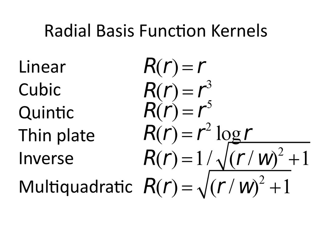
25. Radial Basis Function Kernels

Linear
Cubic
Quintic
Thin plate
Inverse
Multiquadratic
R(r) r
3
R(r) r
5
R(r) r
2
R(r) r log r
2
R(r) 1 / (r / w) +1
2
R(r) (r / w) +1

26. Solve RBF Interpolation Problem

f (z) åai R( z xi )
For each j, åa i R xj xi yj
(
)
• In 1D: N equations, N unknowns, linear solver.
• In n-D: Denote a i, xi, yi Î Rm
Solve Nm equations in Nm unknowns a i.

27. RBF Summary

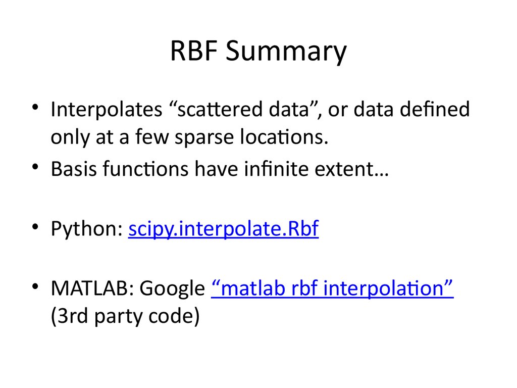
• Interpolates “scattered data”, or data defined
only at a few sparse locations.
• Basis functions have infinite extent…
• Python: scipy.interpolate.Rbf
• MATLAB: Google “matlab rbf interpolation”
(3rd party code)

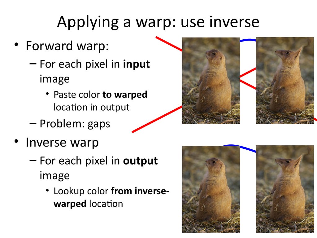
28. Applying a warp: use inverse

• Forward warp:
– For each pixel in input
image
• Paste color to warped
location in output
– Problem: gaps
• Inverse warp
– For each pixel in output
image
• Lookup color from inversewarped location

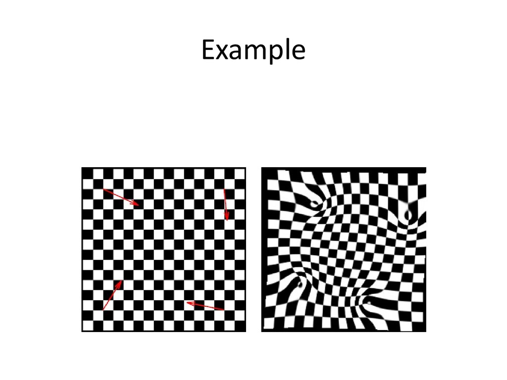
29. Example

30. Example

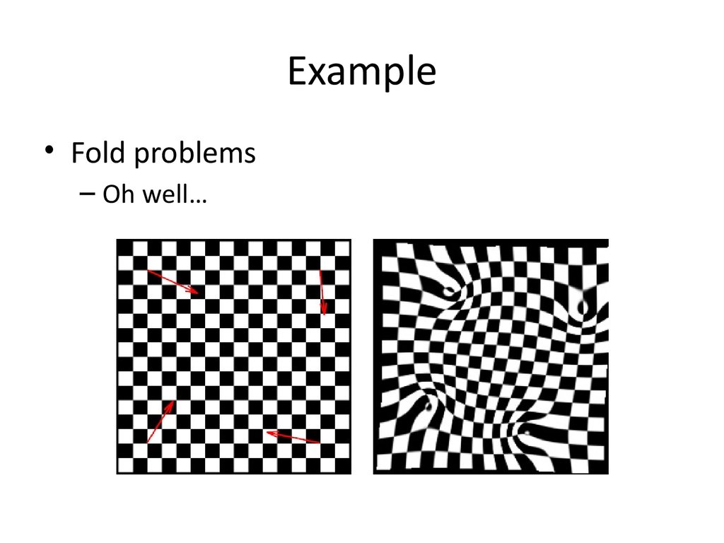
• Fold problems
– Oh well…

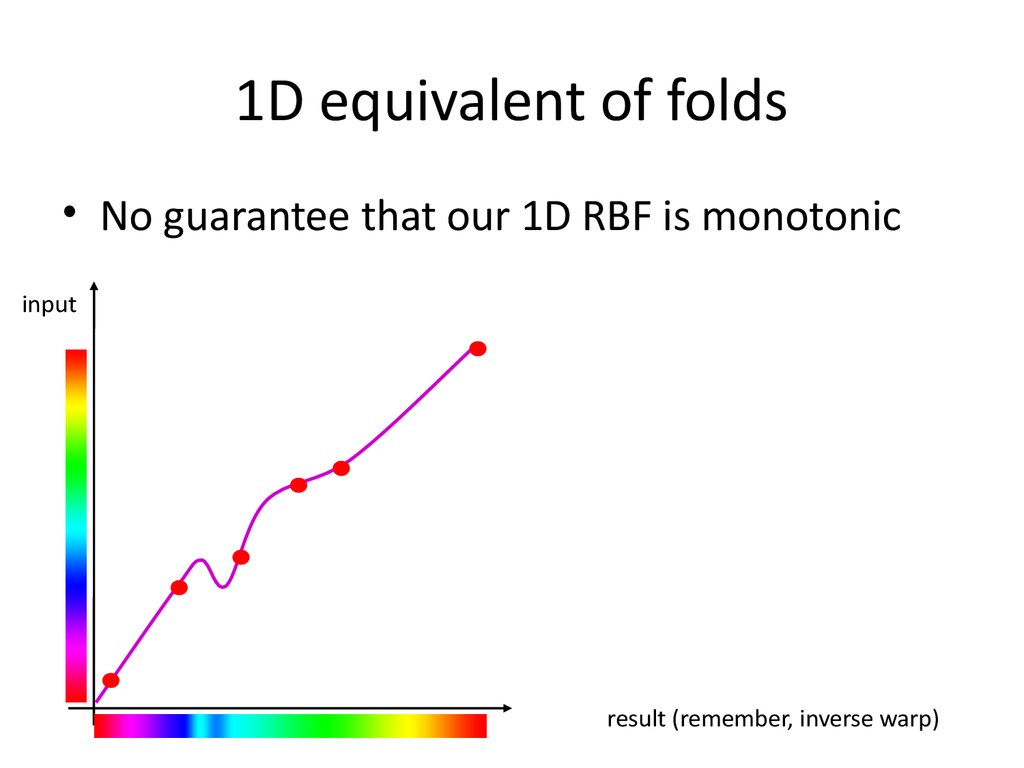
31. 1D equivalent of folds

• No guarantee that our 1D RBF is monotonic
input
result (remember, inverse warp)

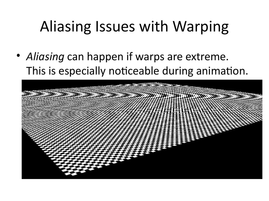
32. Aliasing Issues with Warping

• Aliasing can happen if warps are extreme.
This is especially noticeable during animation.
point sampling
mipmaps & linear interpolation

33. Aliasing Solution

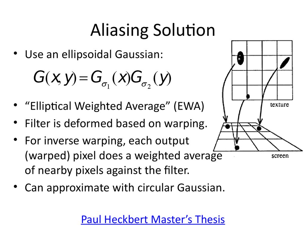
• Use an ellipsoidal Gaussian:
G(x, y) Gs1 (x)Gs 2 (y)
• “Elliptical Weighted Average” (EWA)
• Filter is deformed based on warping.
• For inverse warping, each output
(warped) pixel does a weighted average
of nearby pixels against the filter.
• Can approximate with circular Gaussian.
Paul Heckbert Master’s Thesis

34. Morphing = Object Averaging

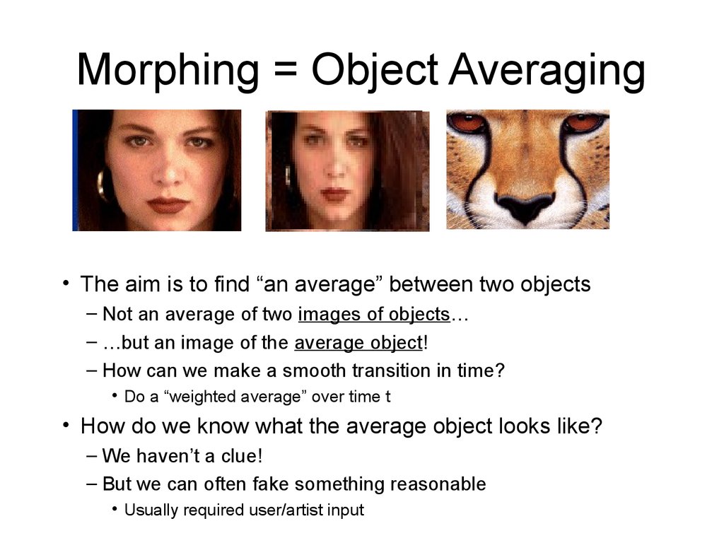
• The aim is to find “an average” between two objects
– Not an average of two images of objects…
– …but an image of the average object!
– How can we make a smooth transition in time?
• Do a “weighted average” over time t
• How do we know what the average object looks like?
– We haven’t a clue!
– But we can often fake something reasonable
• Usually required user/artist input

35. Linear Interpolation

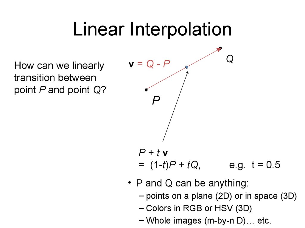
How can we linearly
transition between
point P and point Q?
v=Q-P
Q
P
P+tv
= (1-t)P + tQ,
e.g. t = 0.5
• P and Q can be anything:
– points on a plane (2D) or in space (3D)
– Colors in RGB or HSV (3D)
– Whole images (m-by-n D)… etc.

36. Idea #1: Cross-Dissolve

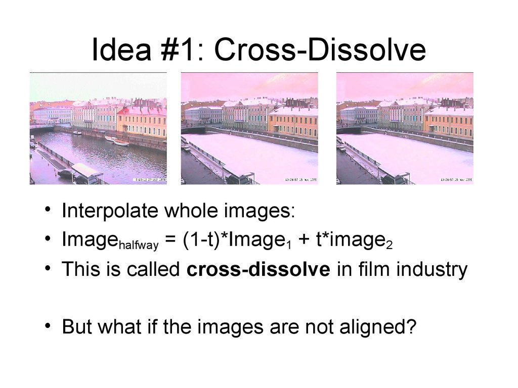
• Interpolate whole images:
• Imagehalfway = (1-t)*Image1 + t*image2
• This is called cross-dissolve in film industry
• But what if the images are not aligned?

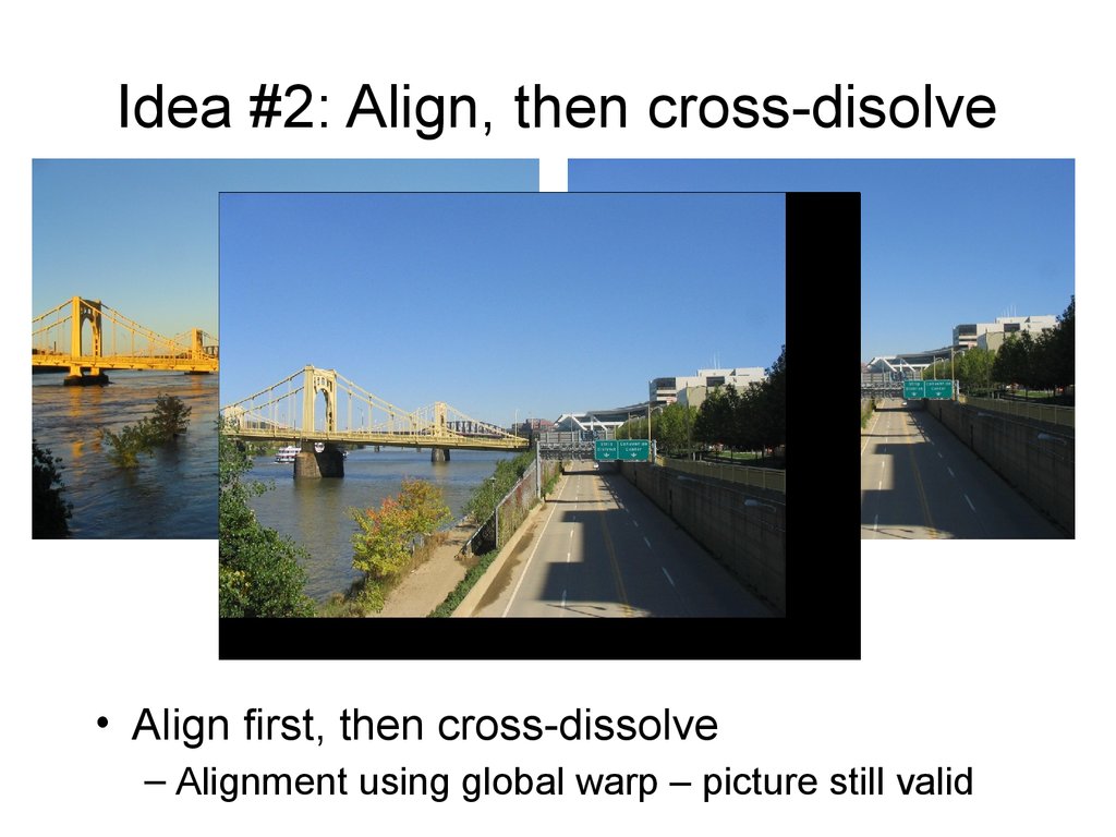
37. Idea #2: Align, then cross-disolve

• Align first, then cross-dissolve
– Alignment using global warp – picture still valid

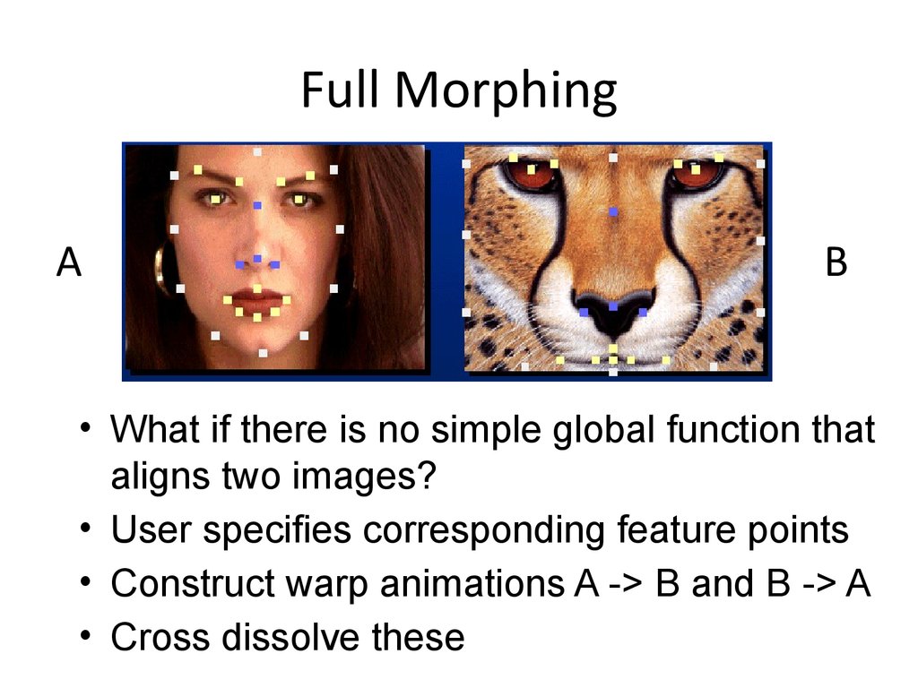
38. Full Morphing

A
B
• What if there is no simple global function that
aligns two images?
• User specifies corresponding feature points
• Construct warp animations A -> B and B -> A
• Cross dissolve these

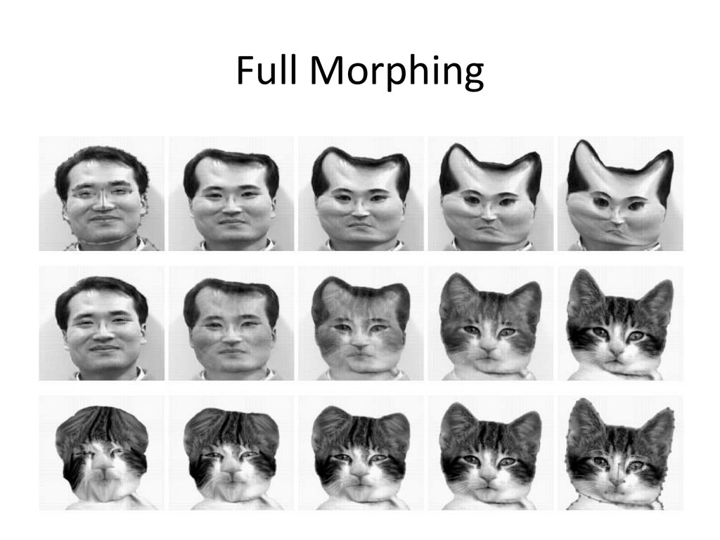
39. Full Morphing

40. Full Morphing

Image A
Full Morphing
Image B
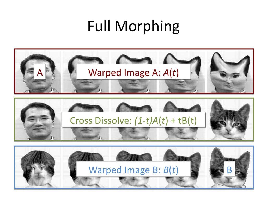
1. Find warping fields from user constraints (points or lines):
Warp field TAB(x, y) that maps A pixel to B pixel
Warp field TBA(x, y) that maps B pixel to A pixel
2. Make video A(t) that warps A over time to the shape of B
Start warp field at identity and linearly interpolate to TBA
Construct video B(t) that warps B over time to shape of A
3. Cross dissolve these two videos.

41. Full Morphing

A
Warped Image A: A(t)
Cross Dissolve: (1-t)A(t) + tB(t)
Warped Image B: B(t)
B

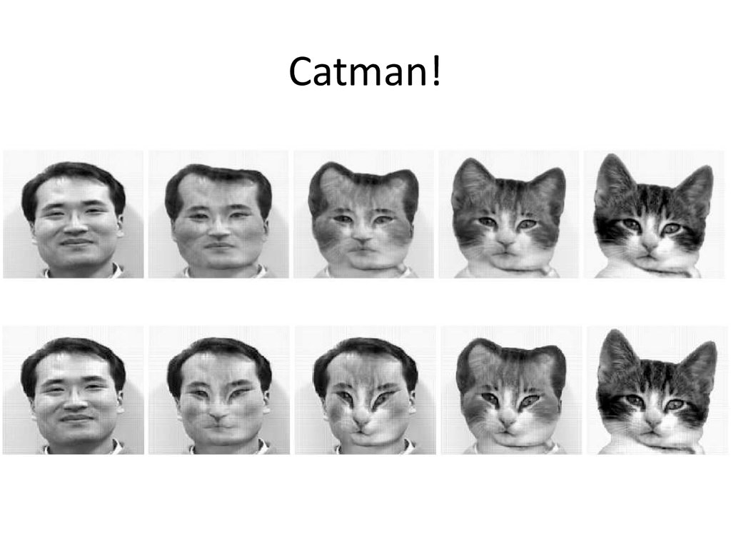
42. Catman!

43. Conclusion

• Illustrates general principle in graphics:
– First register, then blend
• Avoids ghosting
Michael Jackson - Black or White