CS 4700: Foundations of Artificial Intelligence

1. CS 4700: Foundations of Artificial Intelligence

Carla P. Gomes
[email protected]
Module:
SVM
(Reading: Chapter 20.6)
Adapted from Martin Law’s slides
http://www.henrykautz.org/ai/intro_SVM_new.ppt
Carla P. Gomes
CS4700

2. Support Vector Machines (SVM)

Supervised learning methods for classification and regression
relatively new class of successful learning methods they can represent non-linear functions and they have an efficient
training algorithm
derived from statistical learning theory by Vapnik and Chervonenkis
(COLT-92)
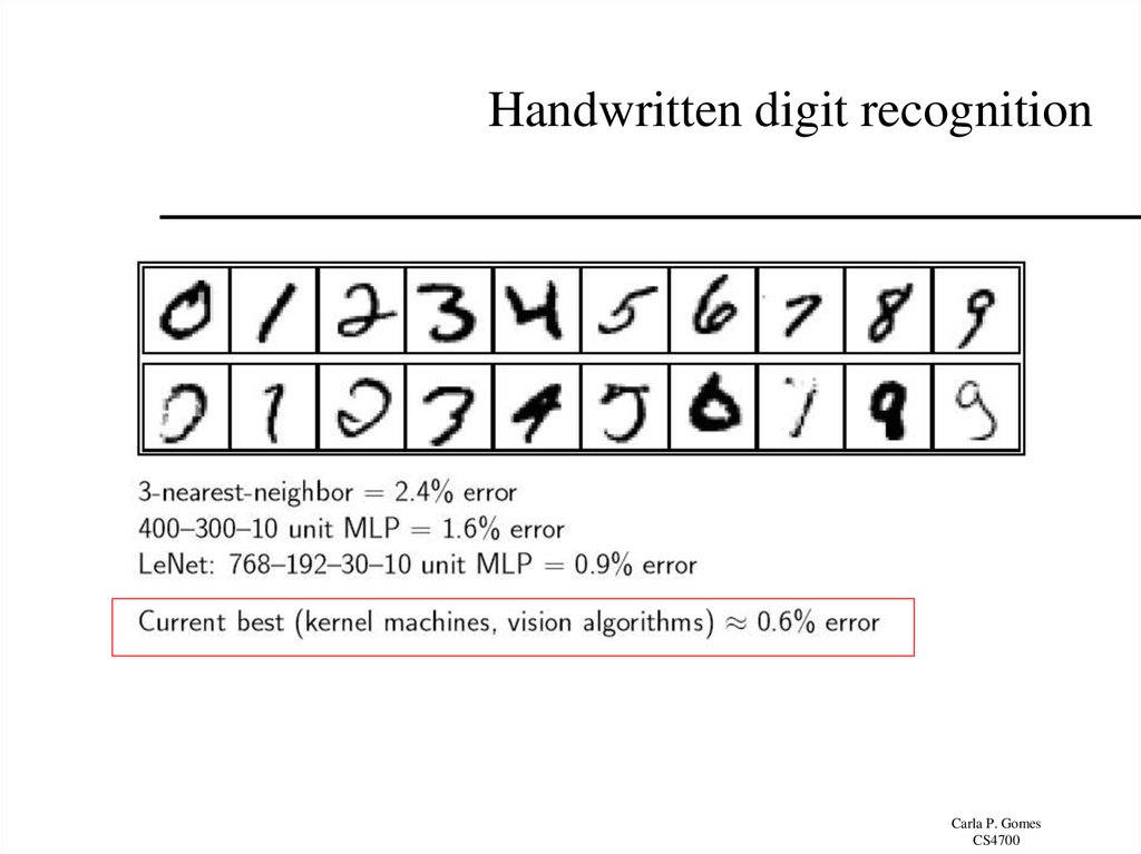
SVM got into mainstream because of their exceptional performance in
Handwritten Digit Recognition
•1.1% error rate which was comparable to a very carefully
constructed (and complex) ANN
Carla P. Gomes
CS4700

3. Two Class Problem: Linear Separable Case

Class 2
Many decision boundaries can
separate these two classes
Which one should we choose?
Class 1
Carla P. Gomes
CS4700

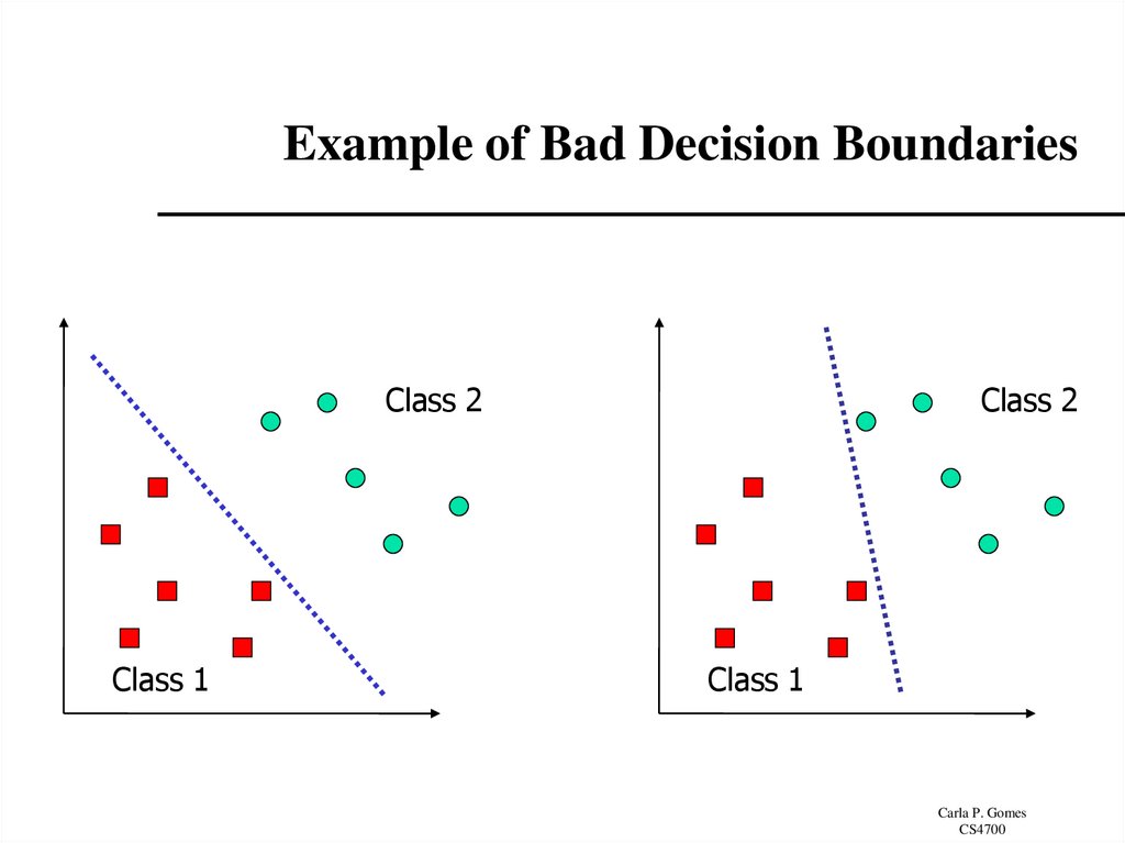
4. Example of Bad Decision Boundaries

Class 2
Class 1
Class 2
Class 1
Carla P. Gomes
CS4700

5. Good Decision Boundary: Margin Should Be Large

The decision boundary should be as far away from the data of both classes
as possible
2
m
– We should maximize the margin, m
w.w
Support vectors
datapoints that the margin
pushes up against
Class 2
Class 1
m
The maximum margin linear
classifier is the linear classifier
with the maximum margin.
This is the simplest kind of
SVM (Called an Linear SVM)
Carla P. Gomes
CS4700

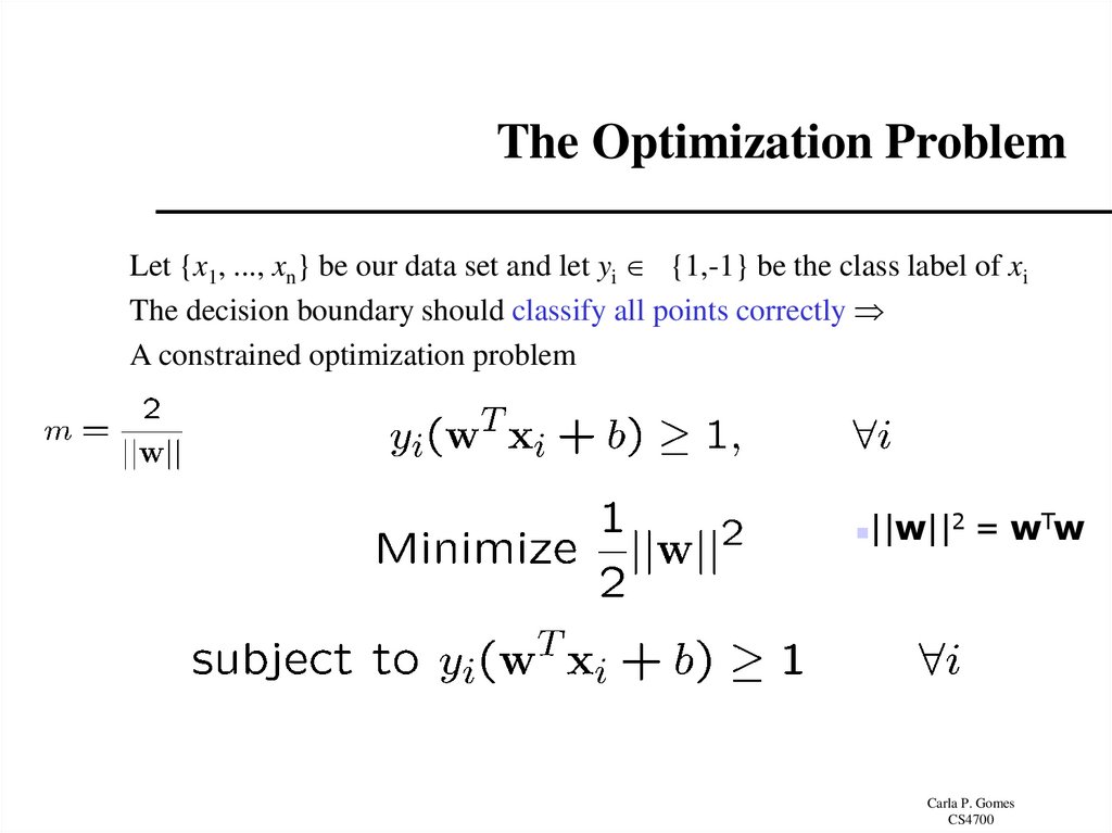
6. The Optimization Problem

Let {x1, ..., xn} be our data set and let yi {1,-1} be the class label of xi
The decision boundary should classify all points correctly
A constrained optimization problem
||w||2 = wTw
Carla P. Gomes
CS4700

7. Lagrangian of Original Problem

The Lagrangian is
Lagrangian multipliers
– Note that ||w||2 = wTw
Setting the gradient of w.r.t. w and b to zero, we have
i 0
Carla P. Gomes
CS4700

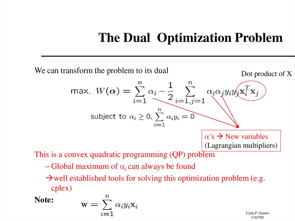
8. The Dual Optimization Problem

We can transform the problem to its dual
Dot product of X
’s New variables
(Lagrangian multipliers)
This is a convex quadratic programming (QP) problem
– Global maximum of i can always be found
well established tools for solving this optimization problem (e.g.
cplex)
Note:
Carla P. Gomes
CS4700

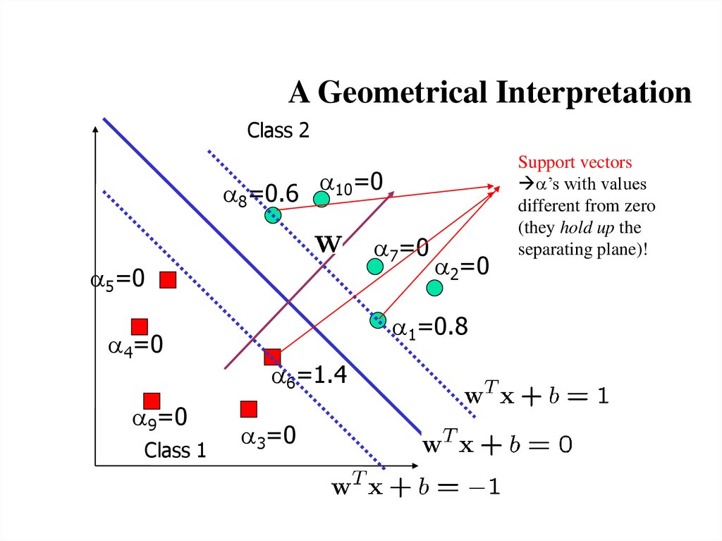
9. A Geometrical Interpretation

Class 2
8=0.6 10=0
7=0
5=0
4=0
9=0
Class 1
2=0
1=0.8
6=1.4
3=0
Support vectors
’s with values
different from zero
(they hold up the
separating plane)!

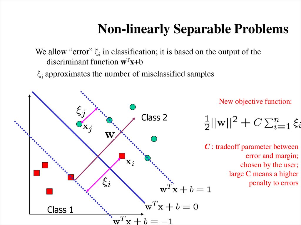
10. Non-linearly Separable Problems

We allow “error” xi in classification; it is based on the output of the
discriminant function wTx+b
xi approximates the number of misclassified samples
New objective function:
Class 2
C : tradeoff parameter between
error and margin;
chosen by the user;
large C means a higher
penalty to errors
Class 1

11. The Optimization Problem

The dual of the problem is
w is also recovered as
The only difference with the linear separable case is that there is an upper
bound C on i
Once again, a QP solver can be used to find i efficiently!!!
Carla P. Gomes
CS4700

12.

Extension to Non-linear SVMs
(Kernel Machines)
Carla P. Gomes
CS4700

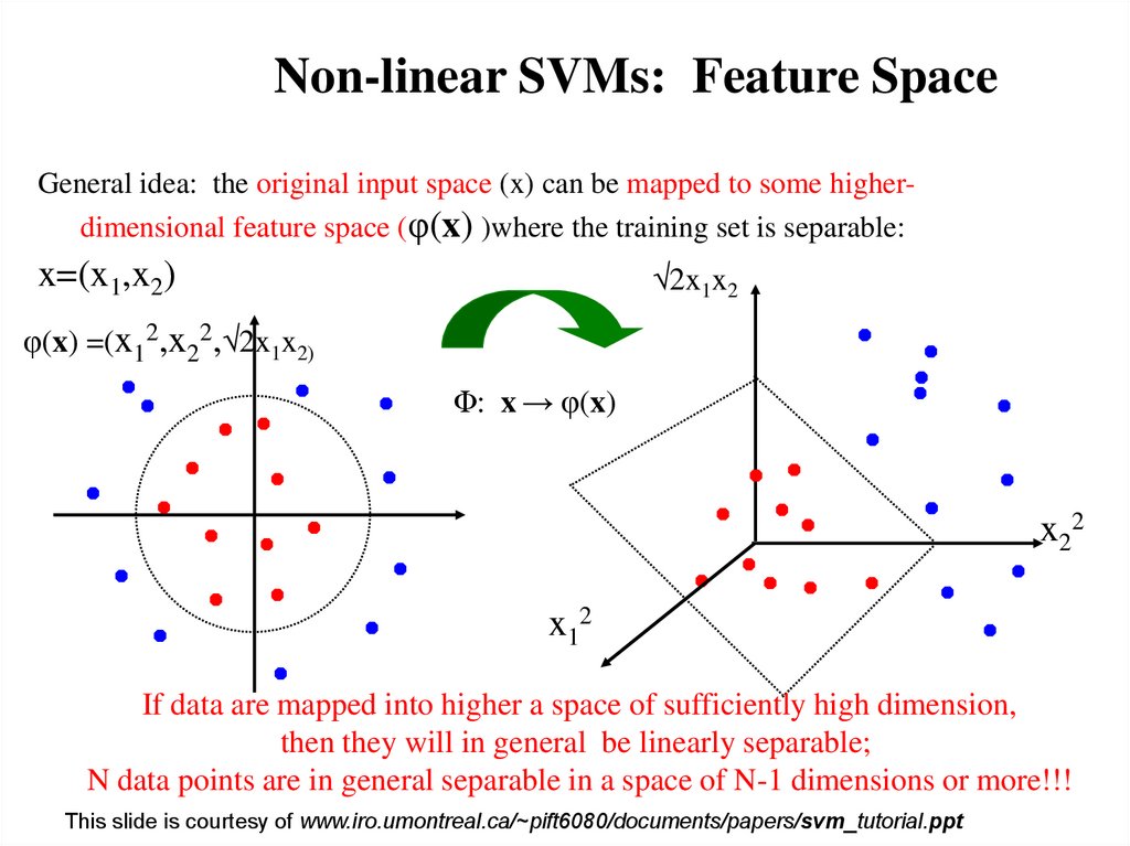
13. Non-Linear SVM

Non-linear SVMs: Feature Space
General idea: the original input space (x) can be mapped to some higherdimensional feature space (φ(x) )where the training set is separable:
2x1x2
x=(x1,x2)
φ(x) =(x12,x22, 2x1x2)
Φ: x → φ(x)
x2 2
x12
If data are mapped into higher a space of sufficiently high dimension,
then they will in general be linearly separable;
N data points are in general separable in a space of N-1 dimensions or more!!!
This slide is courtesy of www.iro.umontreal.ca/~pift6080/documents/papers/svm_tutorial.ppt

14.

Transformation to Feature Space
Possible problem of the transformation
– High computation burden due to high-dimensionality and hard to get a good
estimate
SVM solves these two issues simultaneously
– “Kernel tricks” for efficient computation
– Minimize ||w||2 can lead to a “good” classifier
(.)
Input space
( )
( )
( )
( ) ( ) ( )
( )
( )
( )
( ) ( )
( ) ( )
( )
( ) ( )
( )
( )
Feature space
Carla P. Gomes
CS4700

15. Transformation to Feature Space

Kernel Trick
Note that data only appears as dot products
Recall:
maximize
subject to
N
1 N
i i j yi y j xi x j
2 i j 1
i 1
N
C i 0, i yi 0
i 1
Since data is only represented as dot products, we need not do the mapping explicitly.
Introduce a Kernel Function (*) K such that:
K ( xi , x j ) ( xi ) ( x j )
(*)Kernel function – a function that can be applied to pairs of input data to evaluate dot products
in some corresponding feature space
Carla P. Gomes
CS4700

16. Kernel Trick 

Example Transformation
Consider the following transformation
Define the kernel function K (x,y) as
The inner product (.) (.) can be computed by K without going through
the map (.) explicitly!!!
Carla P. Gomes
CS4700

17. Example Transformation

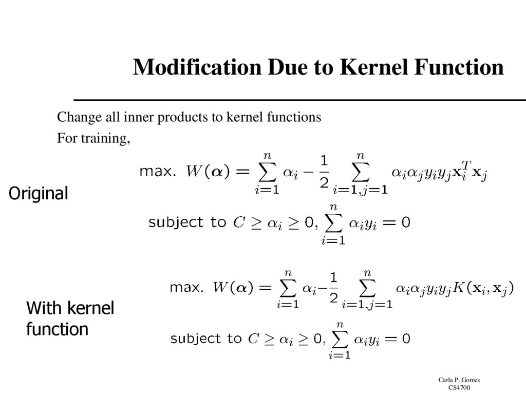
Modification Due to Kernel Function
Change all inner products to kernel functions
For training,
Original
With kernel
function
Carla P. Gomes
CS4700

18. Modification Due to Kernel Function

Examples of Kernel Functions
Polynomial kernel with degree d
Radial basis function kernel with width
– Closely related to radial basis function neural networks
Sigmoid with parameter and
– It does not satisfy the Mercer condition on all and
Research on different kernel functions in different applications is very active
Carla P. Gomes
CS4700

19. Examples of Kernel Functions

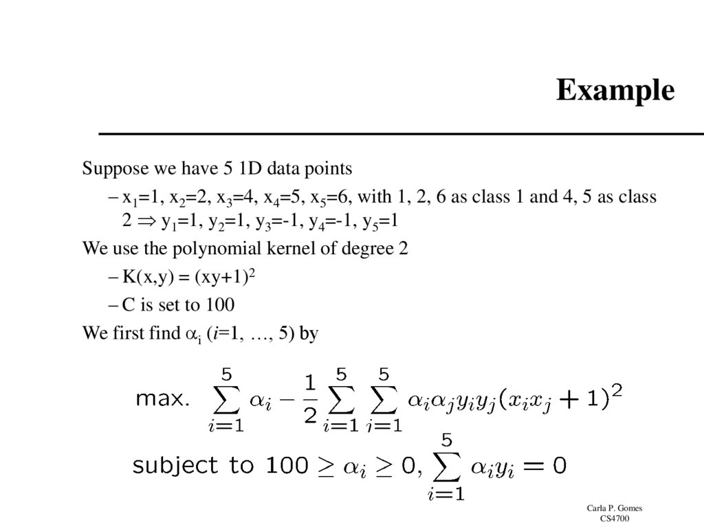
Example
Suppose we have 5 1D data points
– x1=1, x2=2, x3=4, x4=5, x5=6, with 1, 2, 6 as class 1 and 4, 5 as class
2 y1=1, y2=1, y3=-1, y4=-1, y5=1
We use the polynomial kernel of degree 2
– K(x,y) = (xy+1)2
– C is set to 100
We first find i (i=1, …, 5) by
Carla P. Gomes
CS4700

20. Example

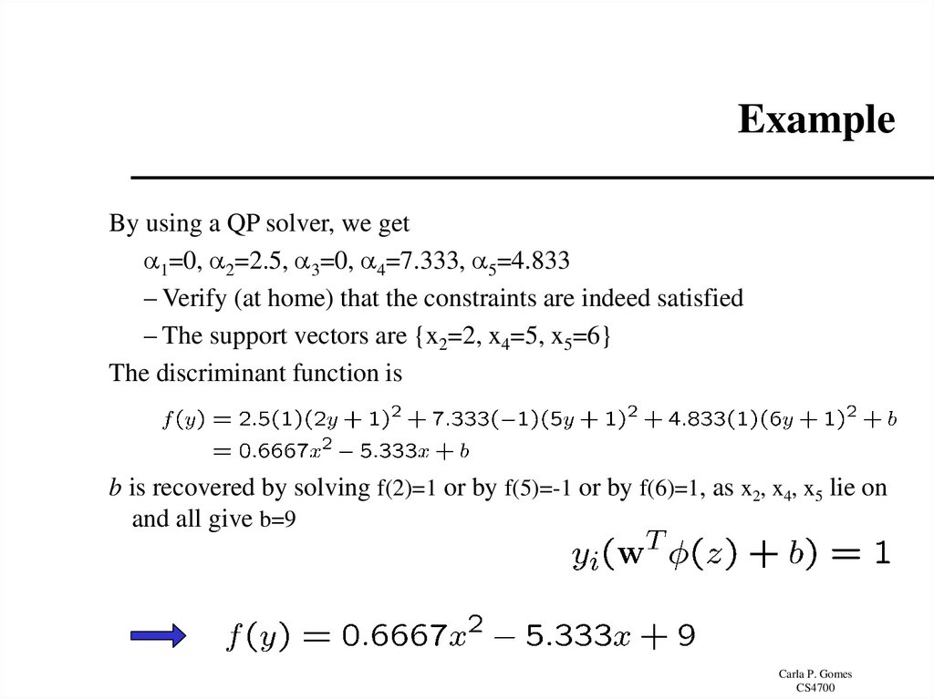
By using a QP solver, we get
1=0, 2=2.5, 3=0, 4=7.333, 5=4.833
– Verify (at home) that the constraints are indeed satisfied
– The support vectors are {x2=2, x4=5, x5=6}
The discriminant function is
b is recovered by solving f(2)=1 or by f(5)=-1 or by f(6)=1, as x2, x4, x5 lie on
and all give b=9
Carla P. Gomes
CS4700

21. Example

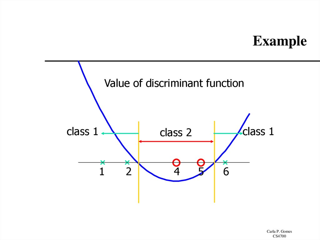
Value of discriminant function
class 1
class 1
class 2
1
2
4
5
6
Carla P. Gomes
CS4700

22. Example

Choosing the Kernel Function
Probably the most tricky part of using SVM.
The kernel function is important because it creates the kernel matrix,
which summarizes all the data
Many principles have been proposed (diffusion kernel, Fisher kernel,
string kernel, …)
There is even research to estimate the kernel matrix from available
information
In practice, a low degree polynomial kernel or RBF kernel with a
reasonable width is a good initial try
Note that SVM with RBF kernel is closely related to RBF neural
networks, with the centers of the radial basis functions automatically
chosen for SVM
Carla P. Gomes
CS4700

23. Choosing the Kernel Function

Software
A list of SVM implementation can be found at http://www.kernelmachines.org/software.html
Some implementation (such as LIBSVM) can handle multi-class
classification
SVMLight is among one of the earliest implementation of SVM
Several Matlab toolboxes for SVM are also available
Carla P. Gomes
CS4700

24. Software

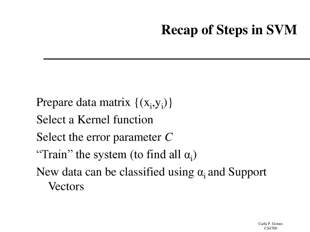
Recap of Steps in SVM
Prepare data matrix {(xi,yi)}
Select a Kernel function
Select the error parameter C
“Train” the system (to find all αi)
New data can be classified using αi and Support
Vectors
Carla P. Gomes
CS4700

25. Recap of Steps in SVM

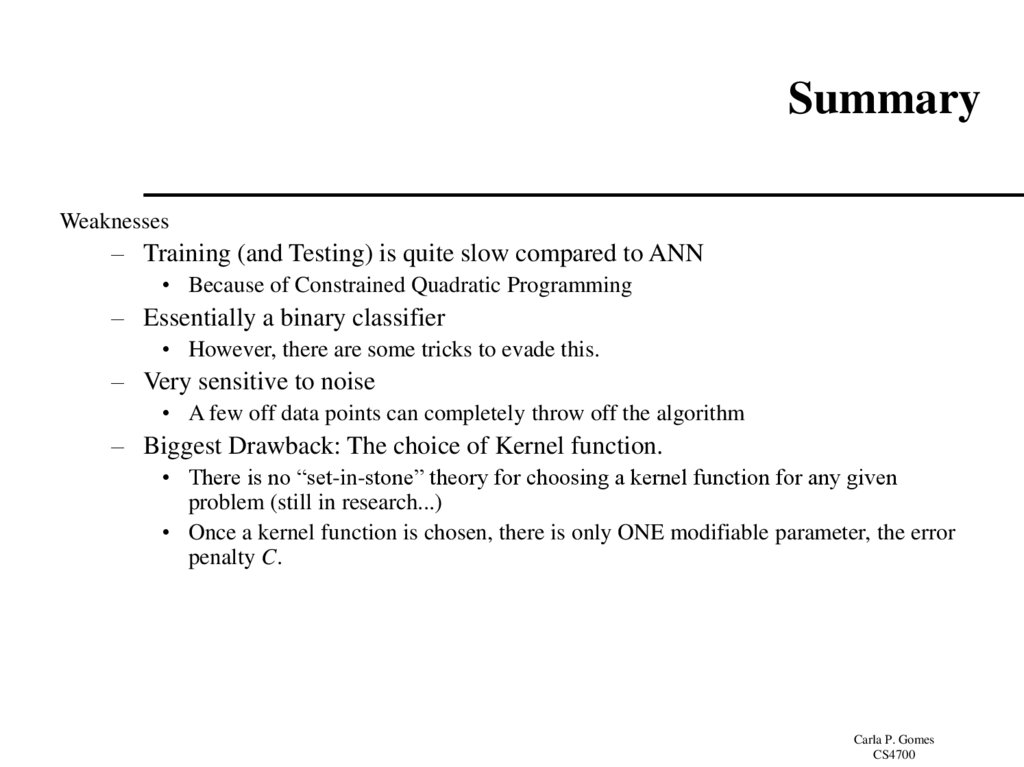
Summary
Weaknesses
– Training (and Testing) is quite slow compared to ANN
• Because of Constrained Quadratic Programming
– Essentially a binary classifier
• However, there are some tricks to evade this.
– Very sensitive to noise
• A few off data points can completely throw off the algorithm
– Biggest Drawback: The choice of Kernel function.
• There is no “set-in-stone” theory for choosing a kernel function for any given
problem (still in research...)
• Once a kernel function is chosen, there is only ONE modifiable parameter, the error
penalty C.
Carla P. Gomes
CS4700

26. Summary

Strengths
– Training is relatively easy
• We don’t have to deal with local minimum like in ANN
• SVM solution is always global and unique (check “Burges” paper for proof and
justification).
– Unlike ANN, doesn’t suffer from “curse of dimensionality”.
• How? Why? We have infinite dimensions?!
• Maximum Margin Constraint: DOT-PRODUCTS!
– Less prone to overfitting
– Simple, easy to understand geometric interpretation.
• No large networks to mess around with.
Carla P. Gomes
CS4700

27. Summary

Applications of SVMs
Bioinformatics
Machine Vision
Text Categorization
Ranking (e.g., Google searches)
Prof. Throsten Joachims
Handwritten Character Recognition
Time series analysis
Lots of very successful applications!!!
Carla P. Gomes
CS4700

28. Applications of SVMs

Handwritten digit recognition
Carla P. Gomes
CS4700

29. Handwritten digit recognition

References
Burges, C. “A Tutorial on Support Vector Machines for Pattern Recognition.”
Bell Labs. 1998
Law, Martin. “A Simple Introduction to Support Vector Machines.” Michigan
State University. 2006
Prabhakar, K. “An Introduction to Support Vector Machines”
Carla P. Gomes
CS4700

30. References

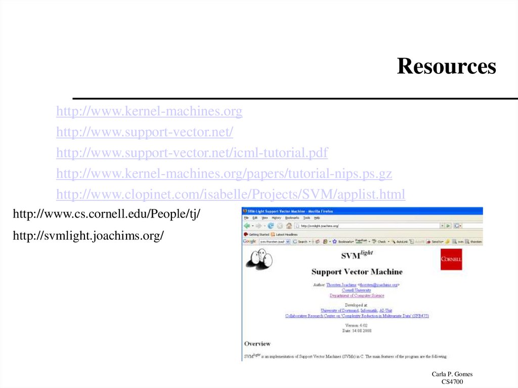
Resources
http://www.kernel-machines.org
http://www.support-vector.net/
http://www.support-vector.net/icml-tutorial.pdf
http://www.kernel-machines.org/papers/tutorial-nips.ps.gz
http://www.clopinet.com/isabelle/Projects/SVM/applist.html
http://www.cs.cornell.edu/People/tj/
http://svmlight.joachims.org/
Carla P. Gomes
CS4700