Real-time PBR Implementation

1.

2.

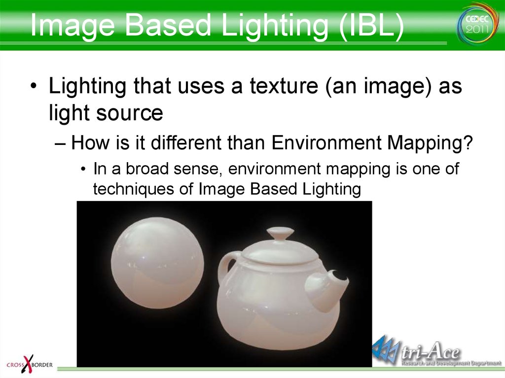
Image Based Lighting (IBL)
• Lighting that uses a texture (an image) as
light source
– How is it different than Environment Mapping?
• In a broad sense, environment mapping is one of
techniques of Image Based Lighting

3.

Physically Based IBL
• Ad-hoc IBL vs. Physically-based IBL
– Has the same differences and similarities
between ad-hoc rendering and physically
based rendering
– Ad-hoc rendering
• Each process needed for rendering is implemented
one by one, ad-hoc
– Physically Based Rendering
• The entire renderer is designed and built based on
physical premises such as the Rendering Equation
and etc.

4.

Physically Based IBL advantages
• Guarantees a rendering result that is close
to shading under punctual light sources
– Materials in a scene dominated by direct
lighting and indirect lighting seem the same
• Consistency is preserved through different lighting
• Artists spend less time tweaking parameters
• Even in a scene dominated by indirect lighting,
materials look realistic
• No need to use an environment map for glossy
objects
– Just add an IBL light source

5.

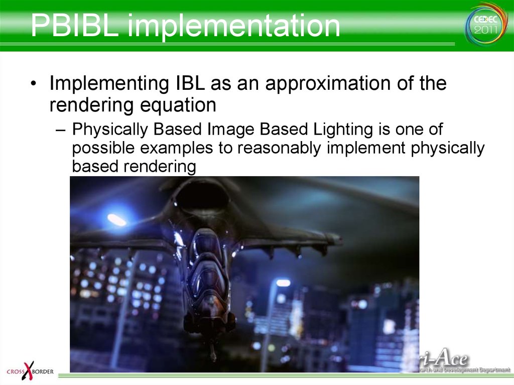
PBIBL implementation
• Implementing IBL as an approximation of the
rendering equation
– Physically Based Image Based Lighting is one of
possible examples to reasonably implement physically
based rendering

6.

Equations
Lo (x, ) f r (x, , ) Li (x, )( n)d
f r (x, , )
Rd
1 F0 (0.0397436shininess 0.0856832)
substitute
shininess
)
| |
max( n , n )
Fspec ( F0 )(n
Fspec ( F0 ) F0 (1 F0 )(1
5
)
| |
5
shininess
) (n
)
F0 (1 F0 )(1
| |
| |
Rd
L (x, )d
Lo (x, ) ( n) 1 F0 (0.0397436 shininess 0.0856832)
i
max( n , n )

7.

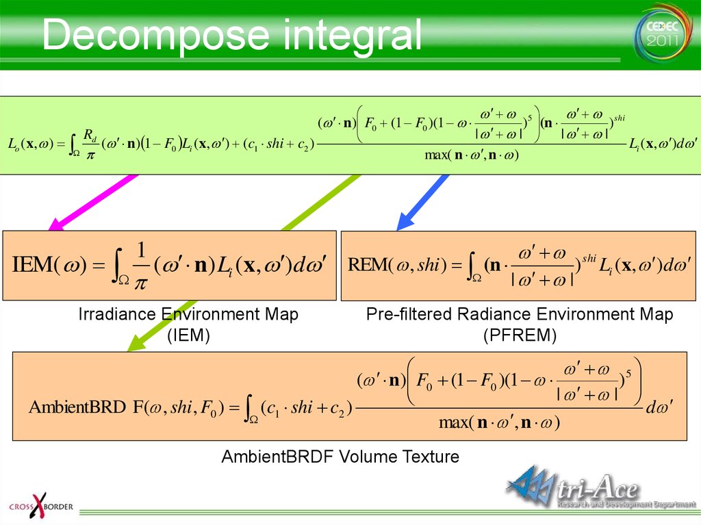
Decompose integral
5
shi
( n) F0 (1 F0 )(1
) (n
)
|
|
|
|
Rd
Lo ( x, )
( n) 1 F0 Li ( x, ) ( c1 shi c2 )
Li ( x, )d
max( n , n )
IEM( )
1
( n) Li (x, )d REM( , shi ) (n
Irradiance Environment Map
(IEM)
shi
) Li (x, )d
| |
Pre-filtered Radiance Environment Map
(PFREM)
5
( n) F0 (1 F0 )(1
)
|
|
d
AmbientBRD F( , shi , F0 ) (c1 shi c2 )
max( n , n )
AmbientBRDF Volume Texture

8.

Implement Ambient BRDF
5
( n) F0 (1 F0 )(1
)
|
|
d
AmbientBRD F( , shi , F0 ) (c1 shi c2 )
max( n , n )
• Precompute this equation off line and store
result to a volume texture
– U – Dot product of eye vector ( ) and normal (n)
– V – shininess
– W – F0

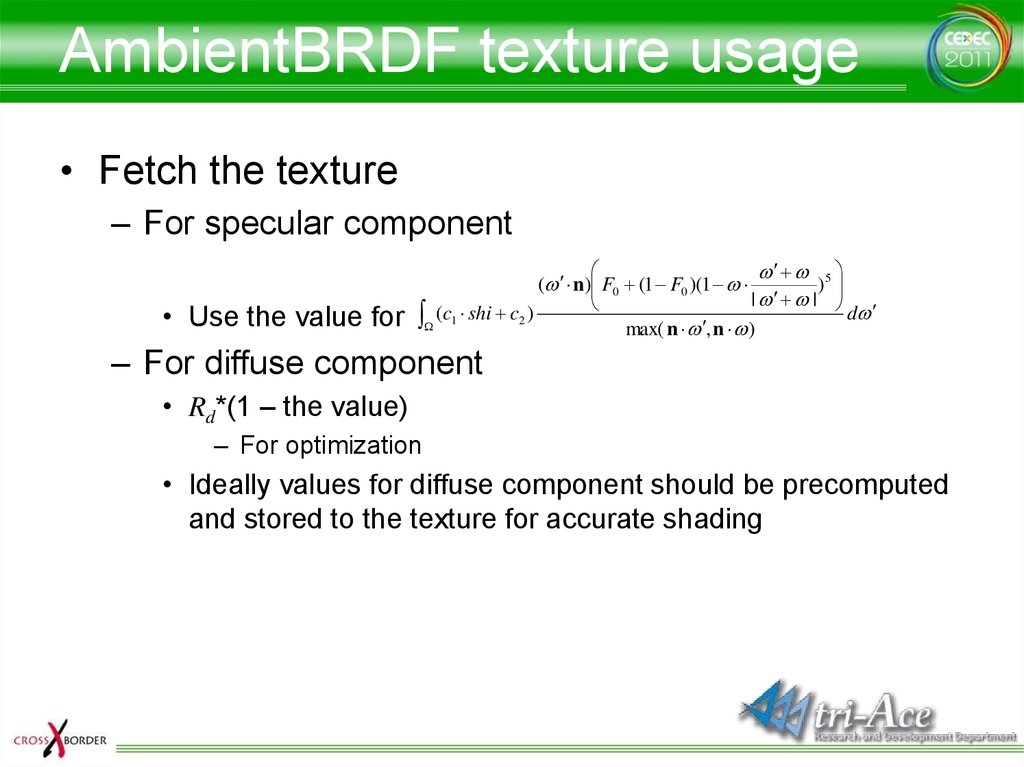
9.

AmbientBRDF texture usage
• Fetch the texture
– For specular component
• Use the value for
5
( n) F0 (1 F0 )(1
)
| |
d
(c1 shi c2 )
max( n , n )
– For diffuse component
• Rd*(1 – the value)
– For optimization
• Ideally values for diffuse component should be precomputed
and stored to the texture for accurate shading

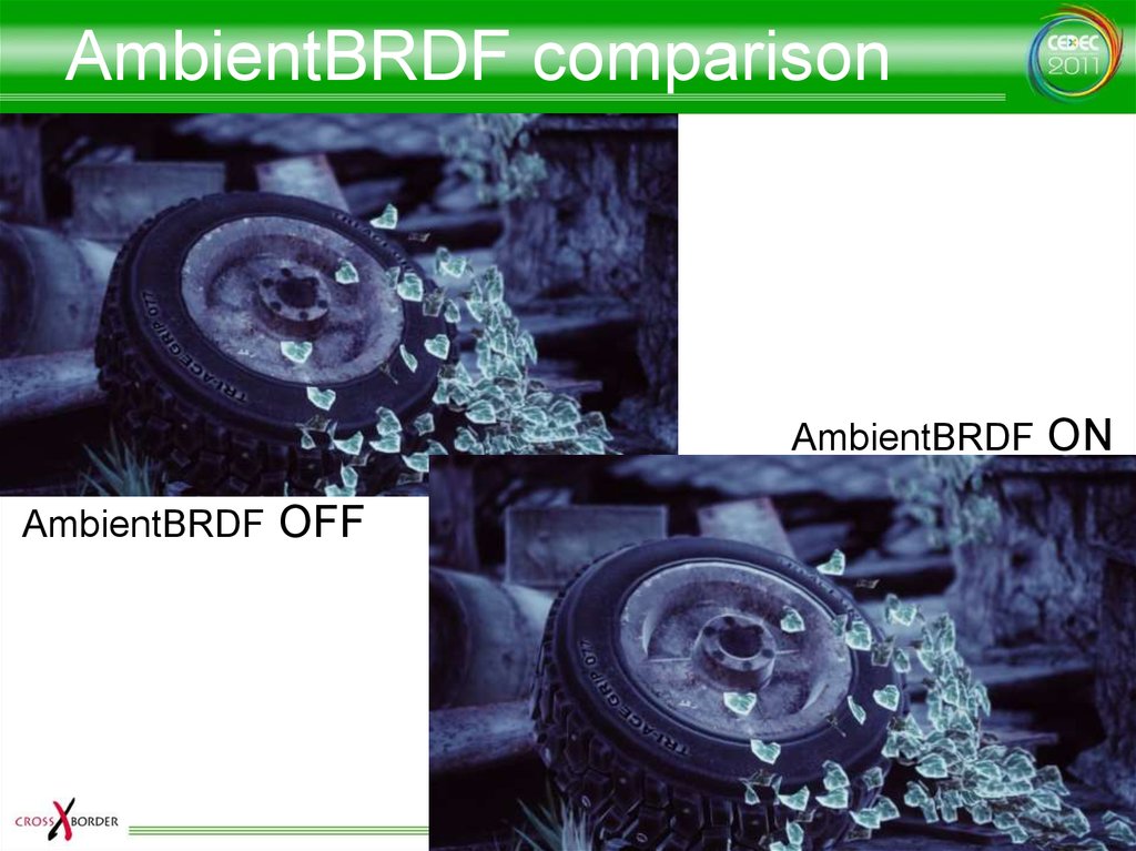
10.

AmbientBRDF comparison
AmbientBRDF ON
AmbientBRDF OFF

11.

Generate textures
• Use AMD CubeMapGen?
– It can't be used for real-time processing on
multi-platform, because it is released as a tool
/ library

12.

Generate textures
• Use AMD CubeMapGen?
– It can't be used for real-time processing on
multi-platform, because it is released as a tool
/ library
But it has become open-source
– Even so, the quality is not perfect and there is
room for improvement

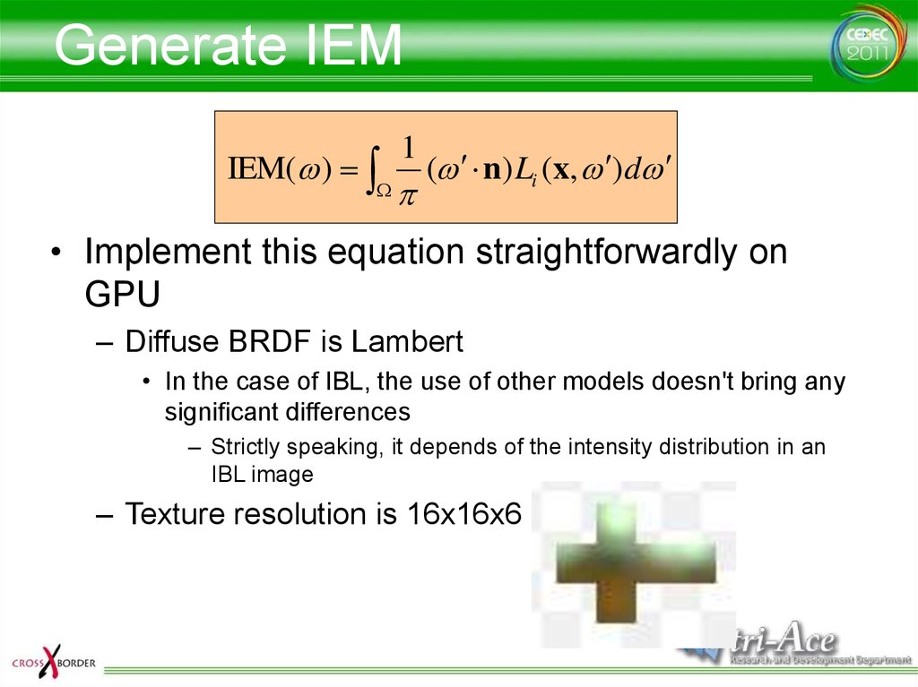
13.

Generate IEM
IEM( )
1
( n) Li (x, )d
• Implement this equation straightforwardly on
GPU
– Diffuse BRDF is Lambert
• In the case of IBL, the use of other models doesn't bring any
significant differences
– Strictly speaking, it depends of the intensity distribution in an
IBL image
– Texture resolution is 16x16x6

14.

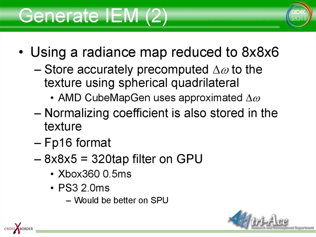
Generate IEM (2)
• Using a radiance map reduced to 8x8x6
– Store accurately precomputed D to the
texture using spherical quadrilateral
• AMD CubeMapGen uses approximated D
– Normalizing coefficient is also stored in the
texture
– Fp16 format
– 8x8x5 = 320tap filter on GPU
• Xbox360 0.5ms
• PS3 2.0ms
– Would be better on SPU

15.

Optimize diffuse term
• Using SH lighting instead of IEM for a high
performance configuration
– Our engine already implements SH lighting
• No extra GPU cost
– Compute the coefficients from 6 texels at the center in
each face
Spherical Harmonics
Irradiance Map

16.

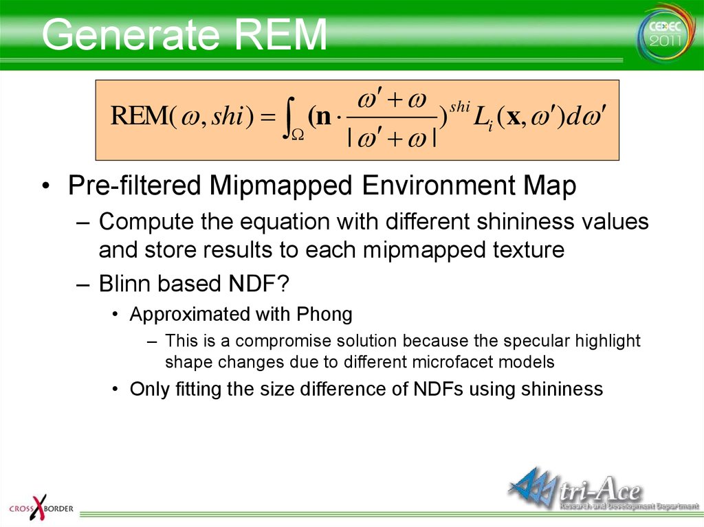
Generate REM
shi
REM( , shi ) (n
) Li (x, )d
| |
• Pre-filtered Mipmapped Environment Map
– Compute the equation with different shininess values
and store results to each mipmapped texture
– Blinn based NDF?
• Approximated with Phong
– This is a compromise solution because the specular highlight
shape changes due to different microfacet models
• Only fitting the size difference of NDFs using shininess

17.

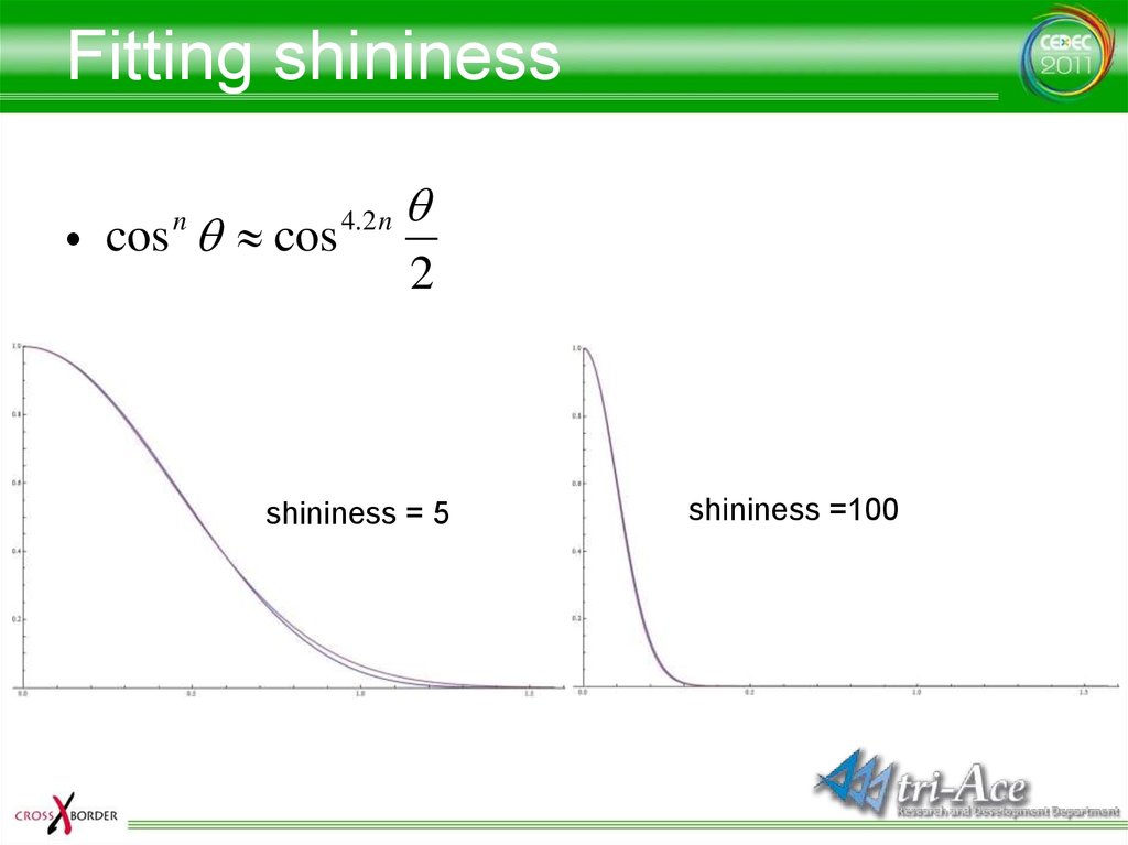
Fitting shininess
• cos cos
n
4 .2 n
2
shininess = 5
shininess =100

18.

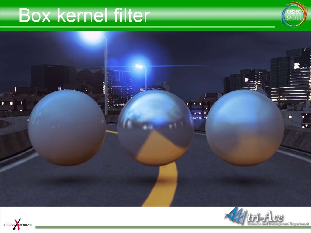
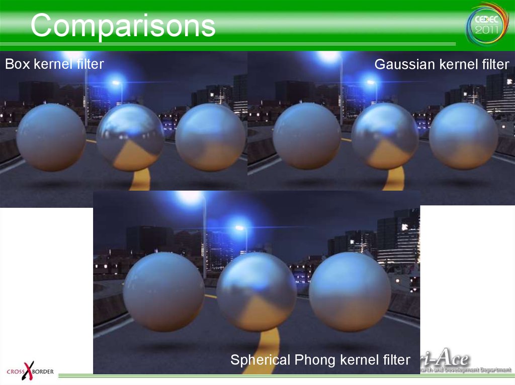
Generate PMREM (1)
• Box-filter kernel filtering
– Simply use bilinear filtering to generate
mipmaps
– LOD values are set according to shininess
• Quality is quite low
• Not even an approximation
– Use as a fastest profile for dynamic PMREM
generation

19.

Box kernel filter

20.

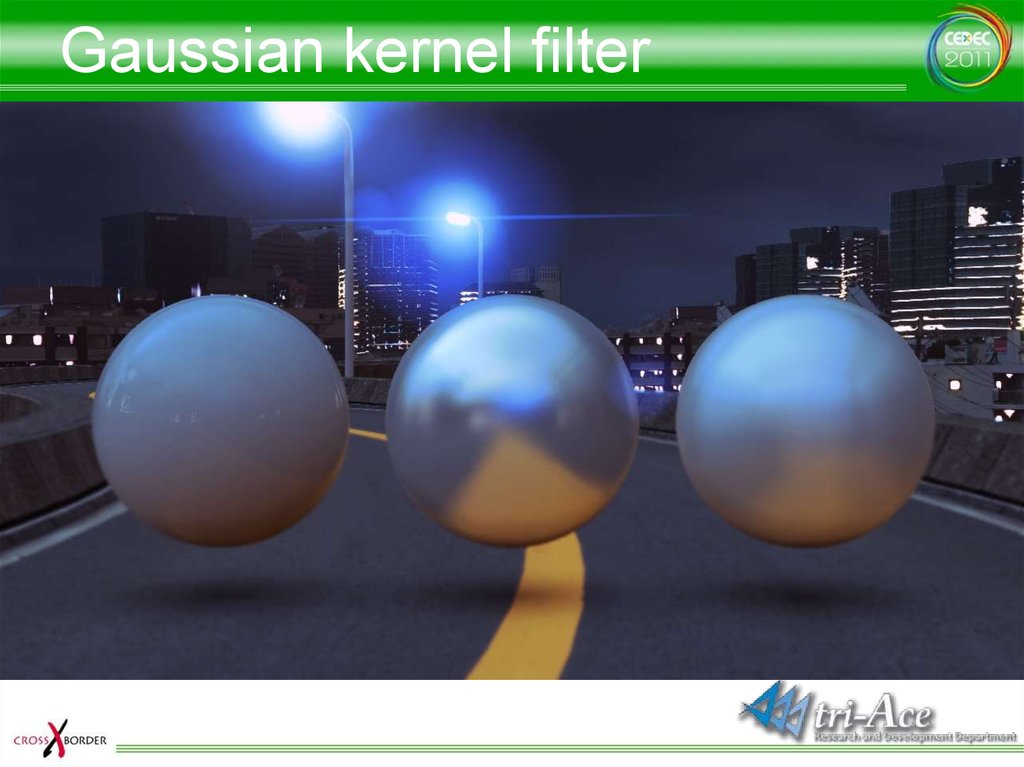
Generate PMREM (2)
• Gaussian kernel filtering
– Apply 2D Gaussian blur to each face
• Not physically based
– As the blur radius increases, visual artifacts from error in
D become noticeable
• The cube map boundary problem is noticeable
– Even using overlapping (described later) for slow
gradation generated by the blur process, since filtering
isn’t performed over edges, banding is perceived on the
edges when colors are changed rapidly
• Use as the second fastest profile for dynamic
PMREM generation

21.

Gaussian kernel filter

22.

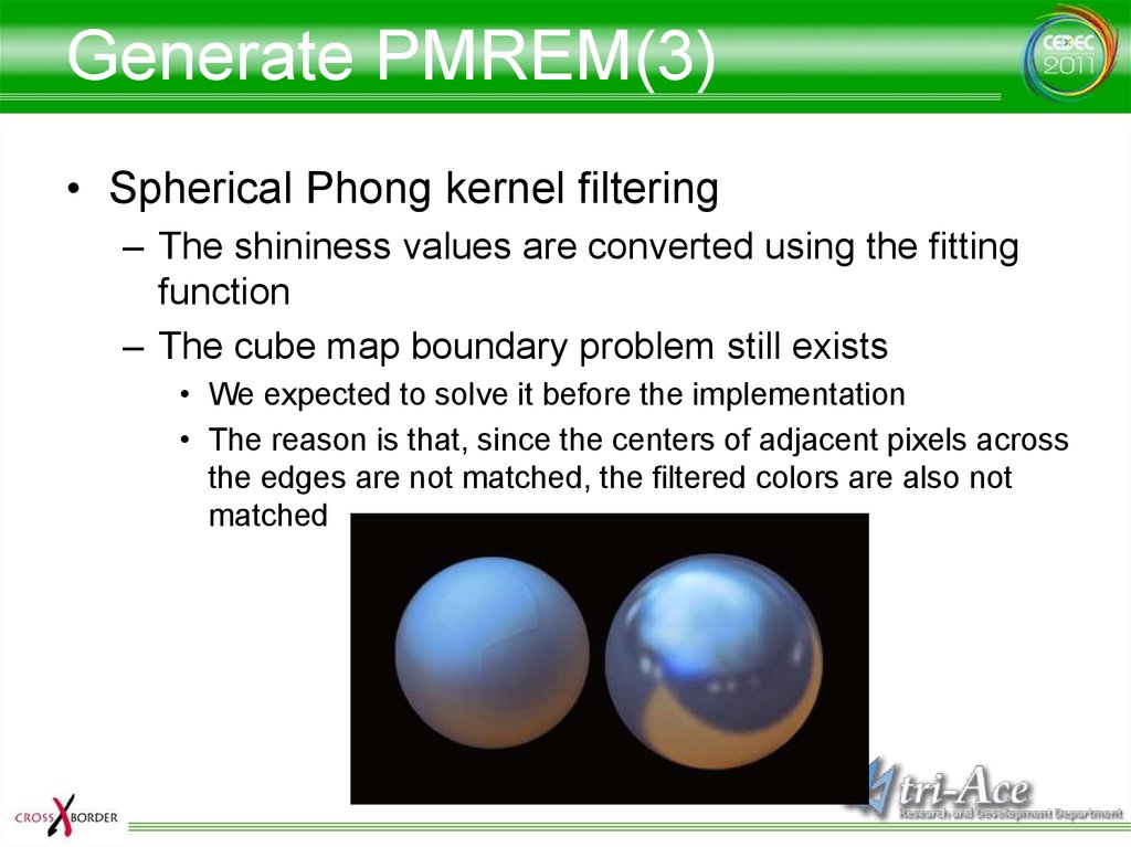
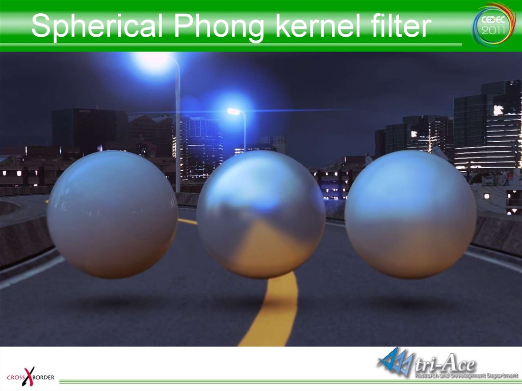
Generate PMREM(3)
• Spherical Phong kernel filtering
– The shininess values are converted using the fitting
function
– The cube map boundary problem still exists
• We expected to solve it before the implementation
• The reason is that, since the centers of adjacent pixels across
the edges are not matched, the filtered colors are also not
matched

23.

Spherical Phong kernel filter

24.

Phong kernel implementation(GPU)
• Brute force implementation similar to
irradiance map generation
– In the final implementation, a face is
subdivided into 9 rectangles for texture fetch
reduction
• Faster by 50%
• 9x6=54 shaders are used for each mip level
– Subdivision is not used below 16x16
• It becomes ALU bound as texture cache efficiently
works for smaller textures

25.

Phong kernel implementation(CPU)
• Offline generation by the tool for static IBL
– SH coefficients and PMREM are automatically
generated during scene export
• For performance, 64x64x6 PMREM is only
supported for static IBL
• Brute force implementation
– All level mipmaps are generated from the top level
texture at the same time
• Core2 8 hardware threads @ 2.8GHz
– 64x64x6 : 5.6s
– 32x32x6 : 0.5s
– SSE & multithread

26.

Generate PFREM (4)
• Poisson kernel filtering
– Implemented a faster version of Phong kernel
filtering
• Apply about 160tap filter with one lower level
mipmap texture
– Quality is compromised even with this process
• Many taps are needed for desired quality
– Didn’t work as optimization
– Didn’t work well with Overlapping process
• Not used because of bad quality and performance

27.

Comparisons
Box kernel filter
Gaussian kernel filter
Spherical
Phong
kernel
filter
Spherical
Phong
kernel
filter

28.

Mipmap LOD
• Mipmap LOD parameter is calculated for
generated PMREM
– Select the mip level according to shininess
• Using texCUBElod() for each pixel
lod a 0.5 log 2 shininess
– a is calculated according to the texture size and shininess
• With trilinear filtering
– Each shininess value corresponding to each mip level is
calculated by fitting
• Fitted for both Box Filter Kernel and Phong Filter Kernel

29.

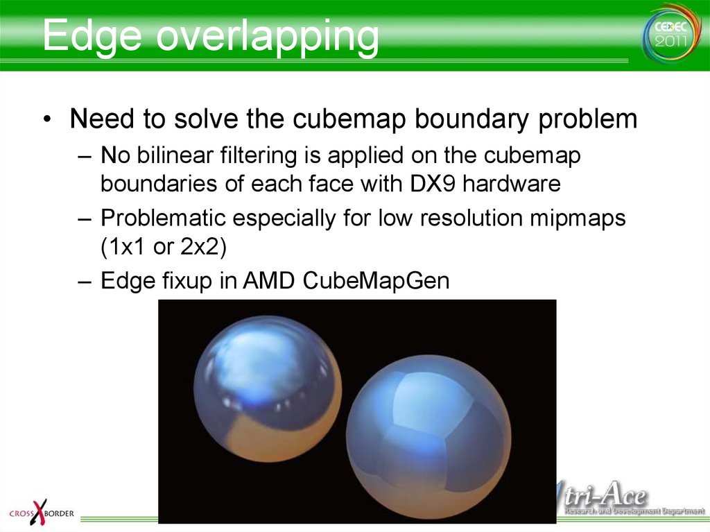
Edge overlapping
• Need to solve the cubemap boundary problem
– No bilinear filtering is applied on the cubemap
boundaries of each face with DX9 hardware
– Problematic especially for low resolution mipmaps
(1x1 or 2x2)
– Edge fixup in AMD CubeMapGen

30.

Edge overlapping (1)
• Blend adjacent boundaries by 50%
– Simplified version of AMD CubeMapGen’s
Edge Fixup
• Adjacent texels across the boundaries become the
same colors
– If corners, the colors become the average of adjacent
three texel colors
– If 1x1, the color becomes the average of all faces
» All texels become the same color
• Banding is still noticeable because color gradation
velocity varies

31.

Edge overlapping (1)

32.

Edge overlapping (2)
• Blend multiple texels
– For the next step, blend 2 texels
• In order to reduce gradation velocity variation,
blend 2 texels by 1/4 and 3/4 ratio
– Same approach as CubeMapGen
– However, banding is still noticeable in the case where
gradation acceleration drastically varies
– As the area where banding is noticeable increases, the
impression gets worse
– Because the blurred area increases, the accuracy of the
integration decreases
» Worse rendering quality

33.

Edge overlapping (3)
• 4 texel blend?
– More blends don’t make sense according to
our research
• 4 texel blending in CubeMapGen is not so high
quality
• Moreover, the precision as a signal decreses

34.

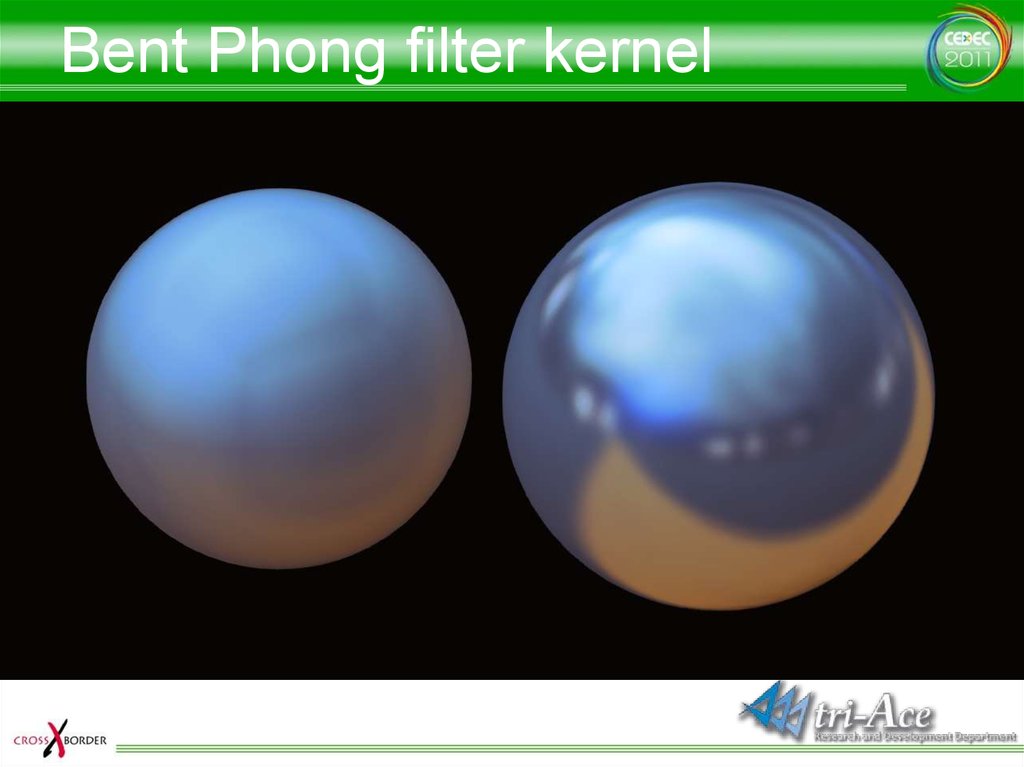
Bent Phong filter kernel
• This algorithm blends normals instead of colors
– Similar to the difference between Gouraud Shading and Phong Shading
• The normal from the center of the cube map through the center of
the texel is bent by an offset angle
– The offset angle is interpolated from zero at the center of the face to a
target angle at the edge
– The target angle is the angle between the two normals of adjacent
faces’ edge texels
• The result from just the above steps was improved, but still not perfect
• Then, using only 50% of target angle gave a much better result
• In the final implementation, the target angle is additionally modified
based on the blur radius
– Large radius : 100% of target angle used
– Small radius : 50% used
– Since optimal values for the target angle are image dependant, adjust
the values by visual adjustment instead of mathematical fitting

35.

Bent Phong filter kernel

36.

Bent Phong filter kernel
Edge overlapping w/ Phong filter kernel
Bent Phong filter kernel

37.

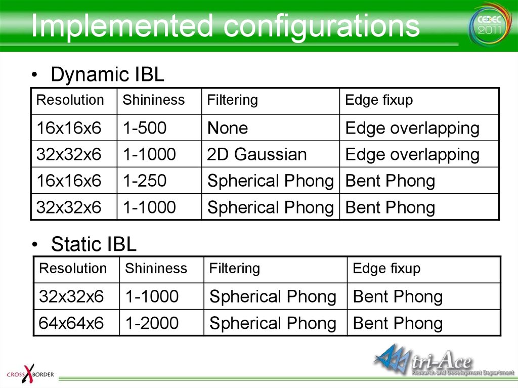
Implemented configurations
• Dynamic IBL
Resolution
Shininess
Filtering
Edge fixup
16x16x6
1-500
None
Edge overlapping
32x32x6
1-1000
2D Gaussian
Edge overlapping
16x16x6
1-250
Spherical Phong Bent Phong
32x32x6
1-1000
Spherical Phong Bent Phong
• Static IBL
Resolution
Shininess
Filtering
Edge fixup
32x32x6
1-1000
Spherical Phong Bent Phong
64x64x6
1-2000
Spherical Phong Bent Phong

38.

Problems with large shininess
• In practice with IBL, materials still look glossy
even with shininess of 1,000 or 2,000
– For mirror like materials, shininess of ten thousands is
preferred
– Difficult to have high enough resolution mipmap
textures, because of memory and performance issues
• Adding the mirror reflection option
– When this functionality is turned
on, the original high resolution
texture is automatically chosen

39.

IBL Blending
• Blending is necessary when using multiple
Image Based Lights
– Implemented blending between an SH light and an
IBL
• Popping was annoying when the blend factor cross 50%
• Not practical
– Blending by fetching Radiance Map twice
• Diffuse term is blended with SH
• For optimization, this process is performed only for the
specified attenuation zone
– Switching shader

40.

IBL Blending

41.

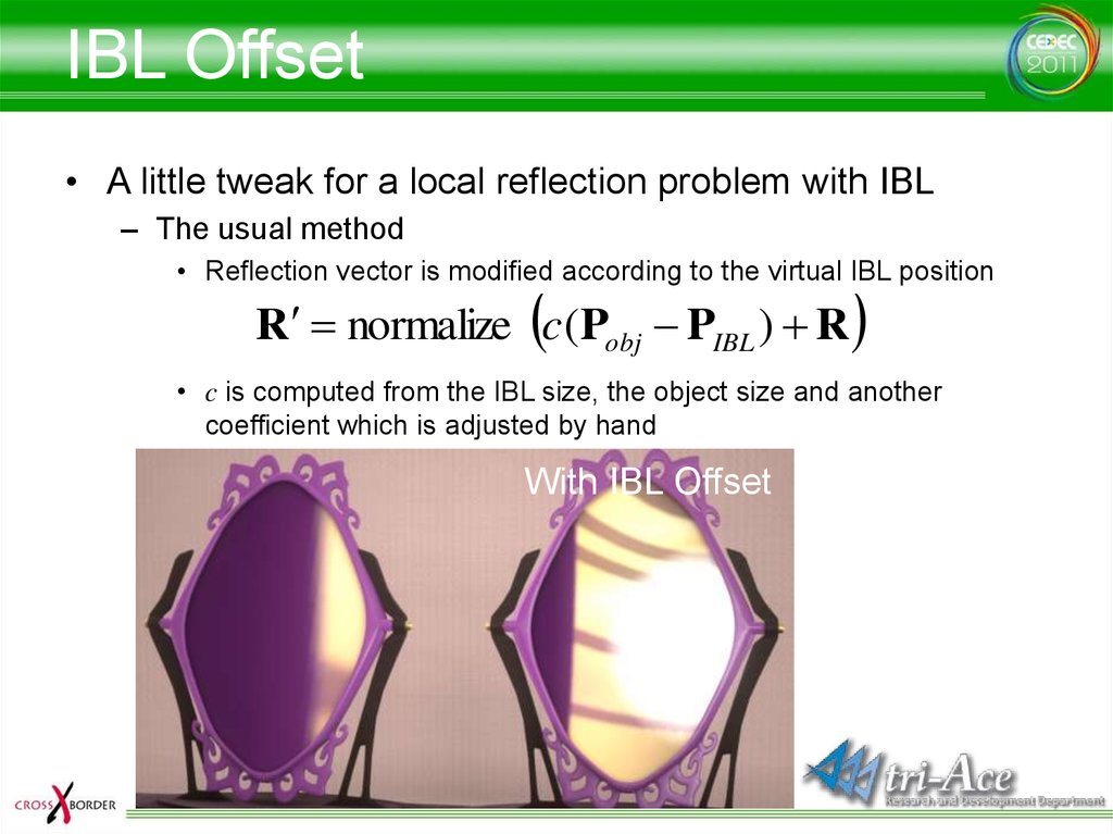
IBL Offset
• A little tweak for a local reflection problem with IBL
– The usual method
• Reflection vector is modified according to the virtual IBL position
R normalize c(Pobj PIBL ) R
• c is computed from the IBL size, the object size and another
coefficient which is adjusted by hand
With IBL Offset

42.

Matching IBL with point light
• In the case where area lighting becomes practical
with IBL, punctual lights becomes problematic
– When adjusting specular for punctual lights, artists tend
to set smaller (blurrier) shininess values than physically
based values
• But it is too blurry for IBL
• When adjusted for IBLs, it is too sharp for punctual lights
– No way for artists to adjust specular without matching

43.

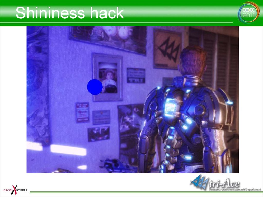
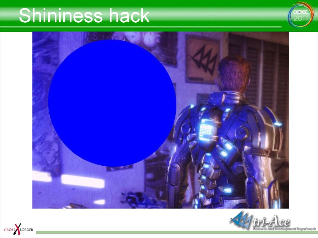
Shininess hack
• Not mathematical matching, but matching the result from
punctual lights to the result from IBL
– Anyhow, this is a hack
• The coefficient can’t be precisely adjusted
– Depends on the shape of the object lit
– Depends on the size of the light source
– Shininess value is compensated by the lighting attenuation factor
• In the case of distant light source, shininess value tends to be the
original shininess value
• In the case of close light source, shininess values tends to be smaller
than the original value
shinines s shininess (saturate(
60
(1 attenuation _ factor)) 2
light _ size

44.

Shininess hack

45.

Shininess hack

46.

HDR IBL Artifact
• The rendering result looks unnatural when the
high intensity light that should be occluded is
coming from grazing angles
– Generally multiply by the ambient occlusion factor
• Enough for LDR IBL
– The artifact is noticeable when HDR IBL has a big
difference of intensities, just like the real world
• Multiplying by the ambient occlusion factor isn’t enough

47.

HDR IBL Artifact

48.

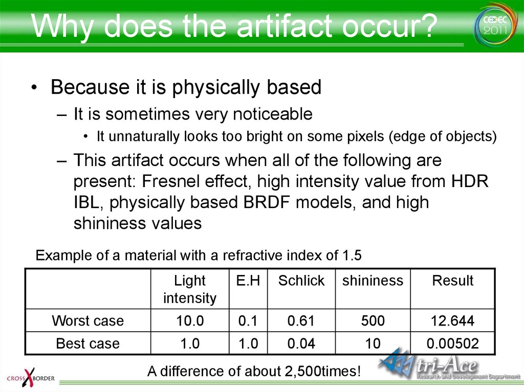
Why does the artifact occur?
• Because it is physically based
– It is sometimes very noticeable
• It unnaturally looks too bright on some pixels (edge of objects)
– This artifact occurs when all of the following are
present: Fresnel effect, high intensity value from HDR
IBL, physically based BRDF models, and high
shininess values
Example of a material with a refractive index of 1.5
Light
intensity
E.H
Schlick
shininess
Result
Worst case
10.0
0.1
0.61
500
12.644
Best case
1.0
1.0
0.04
10
0.00502
A difference of about 2,500times!

49.

Multiplying by AO factor
• Is not enough
– Enough for LDR IBL and non physically based
• Unnoticeable
– Not enough for HDR IBL and physically based
at all
• If an AO factor is 0.1,
– 12.64*0.1=1.264 with the example
– Still higher than 1.0
– Need a more aggressive occlusion factor

50.

Novel Occlusion Factor
• Need almost zero for occluded cases
– Not enough with 0.3 or 0.1 for HDR
• Need 0.01 or less
– Very small values for not occluded area are
problematic
– Need to compute an occlusion term designed
for the specular component
• High-order SH?
• No more extra parameters!

51.

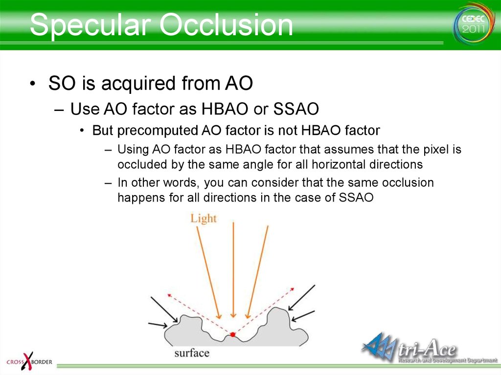
Specular Occlusion
• SO is acquired from AO
– Use AO factor as HBAO or SSAO
• But precomputed AO factor is not HBAO factor
– Using AO factor as HBAO factor that assumes that the pixel is
occluded by the same angle for all horizontal directions
– In other words, you can consider that the same occlusion
happens for all directions in the case of SSAO

52.

Aqcuire Specular Occlusion
• In the case where a pixel is isotropically occluded from
the horizon without gaps
– AO factor becomes
1
2
0
0
cos sin d d cos 2
– Neither conventional AO nor HBAO
are isotropic for horizontal directions,
but Specular Occlusion forcibly
assumes that it is

53.

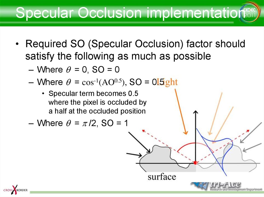
Specular Occlusion implementation
• Required SO (Specular Occlusion) factor should
satisfy the following as much as possible
– Where = 0, SO = 0
– Where = cos-1(AO0.5), SO = 0.5
• Specular term becomes 0.5
where the pixel is occluded by
a half at the occluded position
– Where = /2, SO = 1

54.

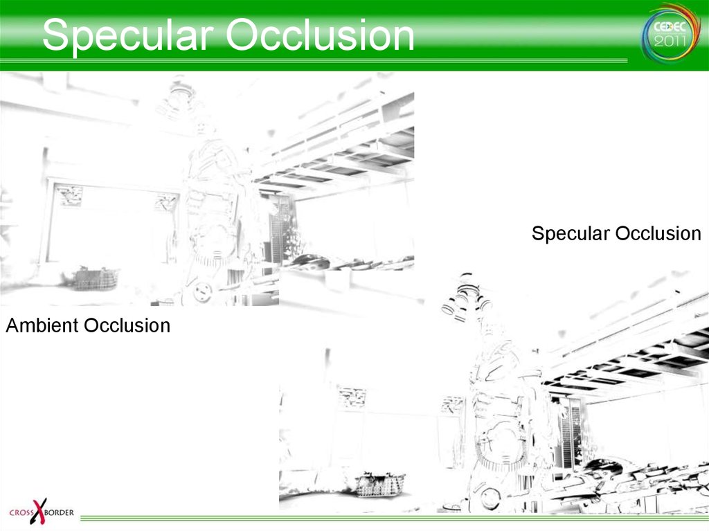
Specular Occlusion
Specular Occlusion
Ambient Occlusion

55.

SO implementation (1)
SO saturate (n E) 2 AO 1
2
• The first equation that satisfies the condition
– Though this satisfies the conditions as Specular
Occlusion, it is not physically based
– Since Specular Occlusion literally represents the
occlusion factor for the specular term, it should be
affected by the shininess value

56.

SO implementation (1)

57.

SO implementation (2)
SO saturate ((n E) AO)0.01shininess 1 AO
• Equation taking into account the shininess value
– More physically based than the first one
– SO suddenly changes with larger shininess values
– High computational cost with Pow
• A little visual contribution to the result
• Smaller occlusion effect than expected

58.

SO implementation (2)

59.

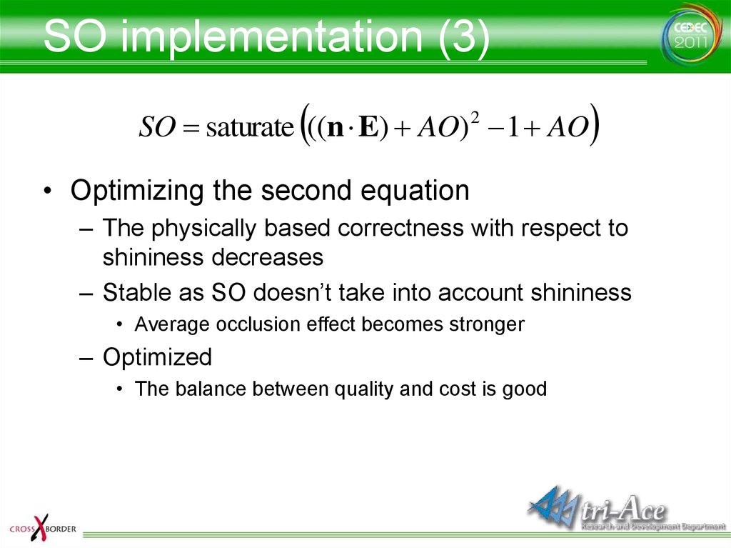
SO implementation (3)
SO saturate ((n E) AO) 2 1 AO
• Optimizing the second equation
– The physically based correctness with respect to
shininess decreases
– Stable as SO doesn’t take into account shininess
• Average occlusion effect becomes stronger
– Optimized
• The balance between quality and cost is good

60.

SO implementation (3)

61.

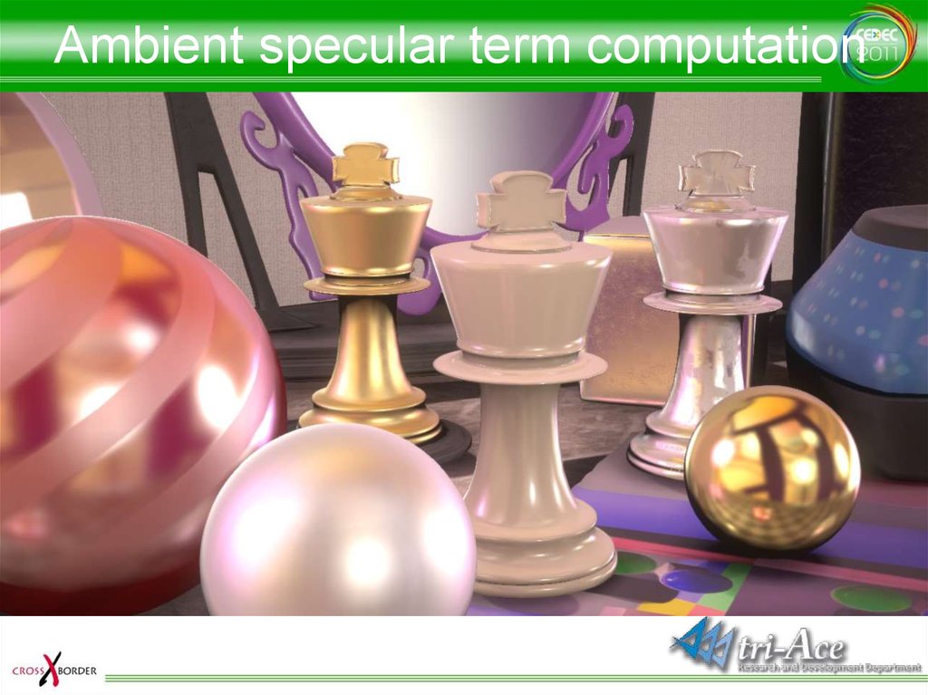
Ambient specular term computation
final specular _ direct specular _ ambient * SO
• Computing the final ambient term
– With this equation, the pixel gets black, because the
occluded pixel isn’t lit by the ambient lights
• In reality, the pixel would be illuminated by the some light
reflected by some of the objects (interreflection)
• The diffuse term has the same issue
– AO itself is not such an aggressive occlusion term
– Diffuse factor does not have such a high dynamic range
– Not problematic
• Problematic for the specular term
– Unnaturally too dark

62.

Ambient specular term computation

63.

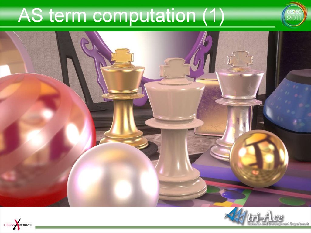
AS term computation (1)
final s _ d lerp( diffuse _ ambient albedo, specular _ ambient , SO)
• Computing pseudo interreflection
– Fundamentally, it should take into account light and albedo at the
reflected point
• Because this implementation is “pseudo”, it takes into account light
and albedo at the shading point
• The results
– Visually, we desired a little more aggressive occlusion effect
• Not based on physics
– Depending on the position, the rendering result becomes strange
• This implementation does not take into account the actual
interreflection

64.

AS term computation (1)

65.

AS term computation (2)
final s _ d lerp( diffuse _ ambient * AO, specular _ ambient , SO)
• Multiplying by the AO factor instead of albedo
– Interreflection like effect becomes smaller, but the
occlusion effect becomes stronger
• Visually preferable
• Eventually, it depends on your preference
• It is a good choice to make this an option for artists

66.

AS term computation (2)

67.

AS term computation (3)
final s _ d AO lerp( diffuse _ ambient AO, specular _ ambient , SO)
• Again, the AO factor is multiplied by the specular
term
– Makes the specular effect for ambient lighting robust
• Not based on physics
• The SO factor itself approximates the approximation
• Relatively adjusted to conservative result
– It also depends on your preference

68.

AS term computation (3)

69.

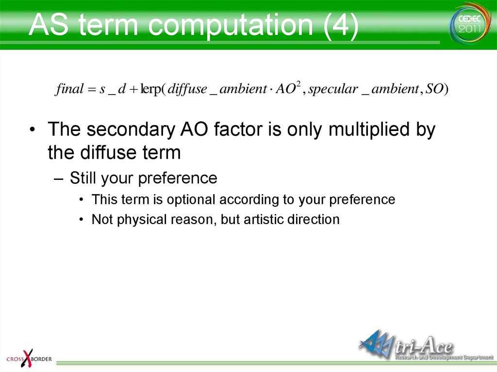
AS term computation (4)
final s _ d lerp( diffuse _ ambient AO2 , specular _ ambient , SO)
• The secondary AO factor is only multiplied by
the diffuse term
– Still your preference
• This term is optional according to your preference
• Not physical reason, but artistic direction

70.

AS term computation (4)
lerp(diffuse _ ambient AO 2 , specular _ ambient , SO )

71.

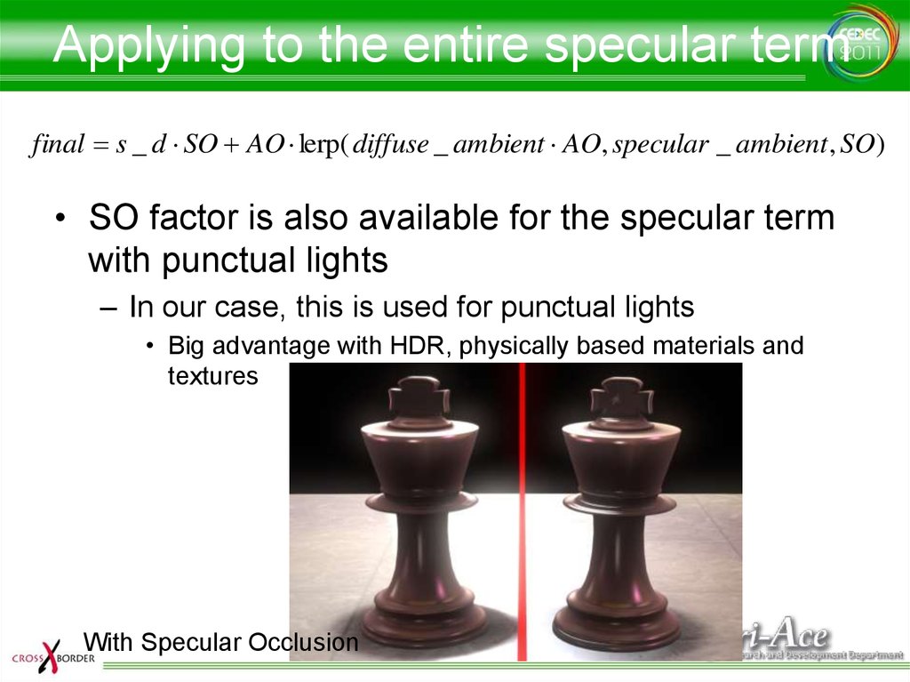
Applying to the entire specular term
final s _ d SO AO lerp( diffuse _ ambient AO, specular _ ambient , SO)
• SO factor is also available for the specular term
with punctual lights
– In our case, this is used for punctual lights
• Big advantage with HDR, physically based materials and
textures
With Specular Occlusion

72.

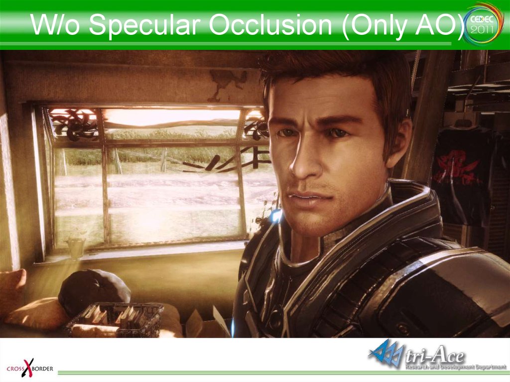
W/o Specular Occlusion (Only AO)

73.

With Specular Occlusion

74.

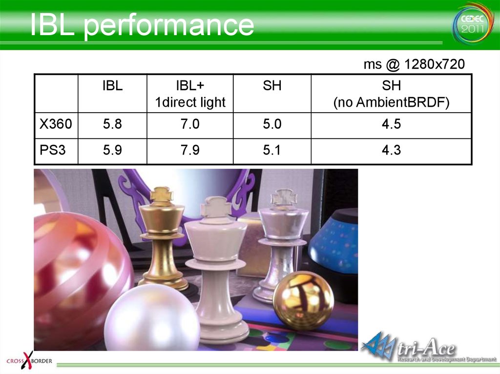
IBL performance
ms @ 1280x720
IBL
IBL+
1direct light
SH
SH
(no AmbientBRDF)
X360
5.8
7.0
5.0
4.5
PS3
5.9
7.9
5.1
4.3

75.

Physically based IBL

76.

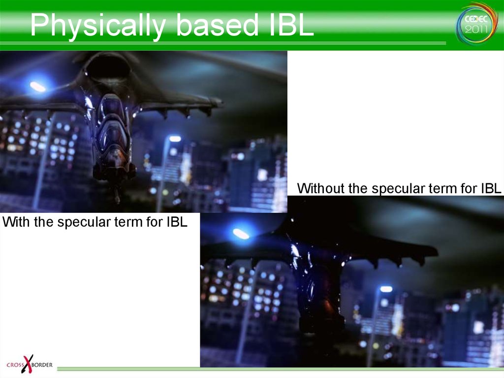
Physically based IBL

77.

Physically based IBL
Without the specular term for IBL
With the specular term for IBL

78.

Conclusion
• When using physically based IBL
– Area lighting which is difficult with punctual
lights becomes feasible
• Soft lighting by a large light source
• Sharp lighting by a small light source
– Consistent material representation with
scenes by either direct and indirect lighting
• Reduce hand adjustment by artists
• Easy to set physically correct parameters to
materials
– True HDR representation becomes possible

79.

Acknowledgements
• R&D department, tri-Ace, Inc.
– Tatsuya Shoji
– Elliott Davis
• Thanks for the English version
– Sébastien Lagarde, Marc Heng
and Naty Hoffman

80.

Questions?
http://research.tri-ace.com