Classifying. Why a separator?

1. CLASSIFYING

Key Separator Relations
Circulating Load
Tromp Curve

2. Why a separator?

Classifying
Why a separator?
• Open circuit grinding is not very efficient:
• Overgrinding of fines
• Useless for quality
• Coating
• No way to be sure of coarse rejects
• Limitation of mill ventilation
• Solution = separator
• Quick grinding is followed by extraction of the fines
already produced, rejects going back to mill inlet
• Retention time in the mill is reduced (20 to 5 min)
• Direct actuator on finish product fineness
KUJ - July 2012 – Grinding I - 2

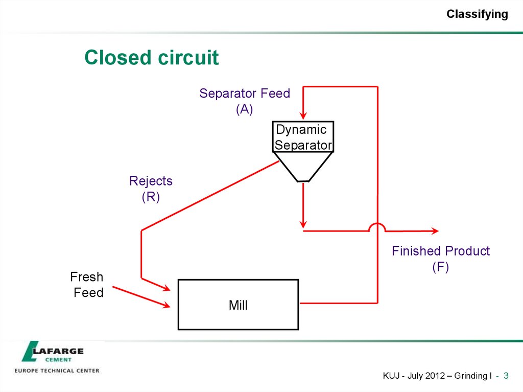
3. Closed circuit

Classifying
Closed circuit
Separator Feed
(A)
Dynamic
Separator
Rejects
(R)
Finished Product
(F)
Fresh
Feed
Mill
KUJ - July 2012 – Grinding I - 3

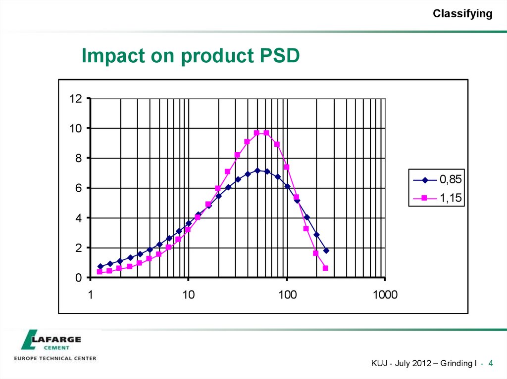
4. Impact on product PSD

Classifying
Impact on product PSD
12
10
8
0,85
0,85
1,15
6
4
2
0
1
10
100
1000
KUJ - July 2012 – Grinding I - 4

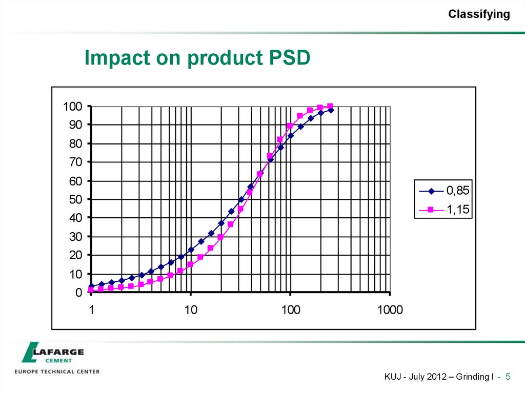
5. Impact on product PSD

Classifying
Impact on product PSD
100
90
80
70
60
0,85
50
1,15
40
30
20
10
0
1
10
100
1000
KUJ - July 2012 – Grinding I - 5

6. Separation in general

Classifying
Separation in general
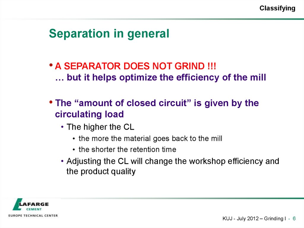
• A SEPARATOR DOES NOT GRIND !!!
… but it helps optimize the efficiency of the mill
• The “amount of closed circuit” is given by the
circulating load
• The higher the CL
• the more the material goes back to the mill
• the shorter the retention time
• Adjusting the CL will change the workshop efficiency and
the product quality
KUJ - July 2012 – Grinding I - 6

7. Circulating Load (CL)

Classifying
Circulating Load (CL)
• How can we determine it?
A: Separator Feed
• C.L. = R/F (used by Lafarge)
• Others define it as C.L. = A/F
• Or A/F = 1+ R/F
• Meaning?
• Number of material passages
through the mill, in addition to the
first one
• What is the best CL?
The best is unique to each
circuit and can only be found
by experimentation
R: Rejects
(or Tails)
F: Fines
KUJ - July 2012 – Grinding I - 7

8. Separation efficiency

Classifying
Separation efficiency
• How do we assess the efficiency of separation?
• The tool is the separation curve, or TROMP CURVE
• First, what do we expect of a separator?
•…
KUJ - July 2012 – Grinding I - 8

9. Separation efficiency

Classifying
Separation efficiency
• What do we expect of a separator?
100%
9
90%
8
80%
7
70%
6
60%
5
50%
4
40%
3
30%
2
20%
1
10%
0
0%
Feed PSD
Feed
Feed Feed
Rejects
Feed
Rejects
Ideal
Rejects
Fines
FinesFines
Ideal
P(x)
Ideal separation
Real separation
Tromp curve
1,
0
1,
3
1,
6
2,
0
2,
5
3,
2
4,
0
5,
0
6,
3
8,
0
110
0,,0
0
112
2,,0
0
116
6,,0
0
220
0,,0
0
225
5,,0
0
332
2,,0
0
440
0,,0
0
5500,
,00
6633,
,00
8800
,,00
10
KUJ - July 2012 – Grinding I - 9

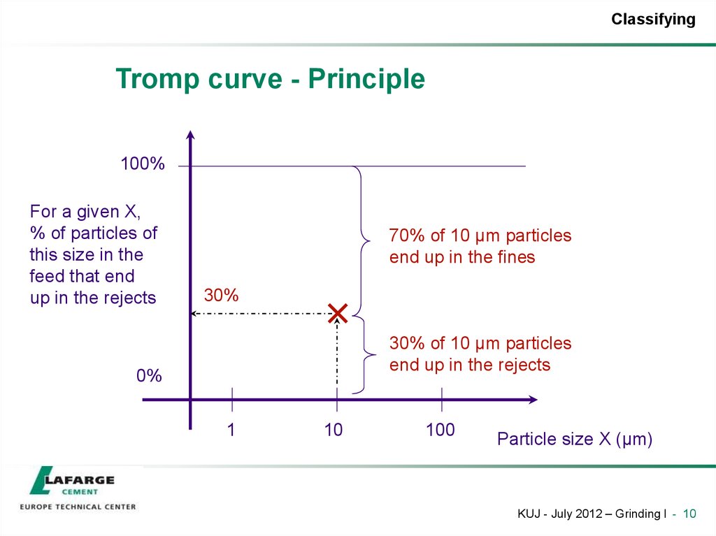
10. Tromp curve - Principle

Classifying
Tromp curve - Principle
100%
For a given X,
% of particles of
this size in the
feed that end
up in the rejects
70% of 10 µm particles
end up in the fines
30%
30% of 10 µm particles
end up in the rejects
0%
1
10
100
Particle size X (µm)
KUJ - July 2012 – Grinding I - 10

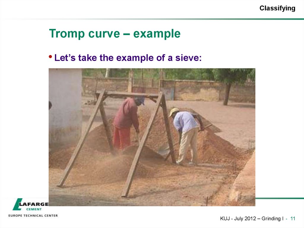
11. Tromp curve – example

Classifying
Tromp curve – example
• Let’s take the example of a sieve:
KUJ - July 2012 – Grinding I - 11

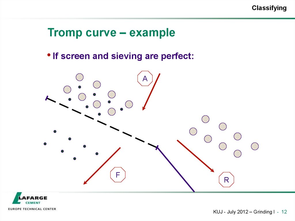
12. Tromp curve – example

Classifying
Tromp curve – example
• If screen and sieving are perfect:
A
F
R
KUJ - July 2012 – Grinding I - 12

13. Tromp curve – Perfect screen

Classifying
Tromp curve – Perfect screen
100%
For a given X,
% of particles of
this size in the
feed that end
up in the rejects
Below 50 µm, all
particles end up in
the fines
Above 50 µm, all
particles end up in
the rejects
0%
1
10
50µm 100
Particle size X (µm)
KUJ - July 2012 – Grinding I - 13

14. By-pass

Classifying
By-pass
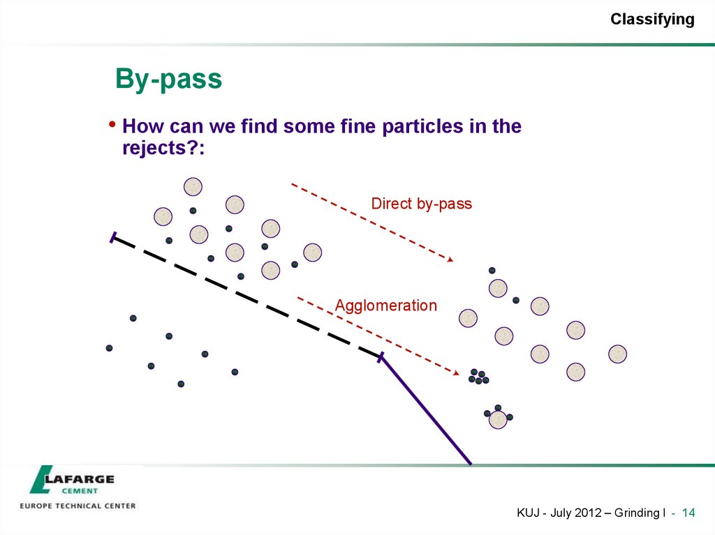
• How can we find some fine particles in the
rejects?:
Direct by-pass
Agglomeration
KUJ - July 2012 – Grinding I - 14

15. Tromp curve – With bypass

Classifying
Tromp curve – With bypass
100%
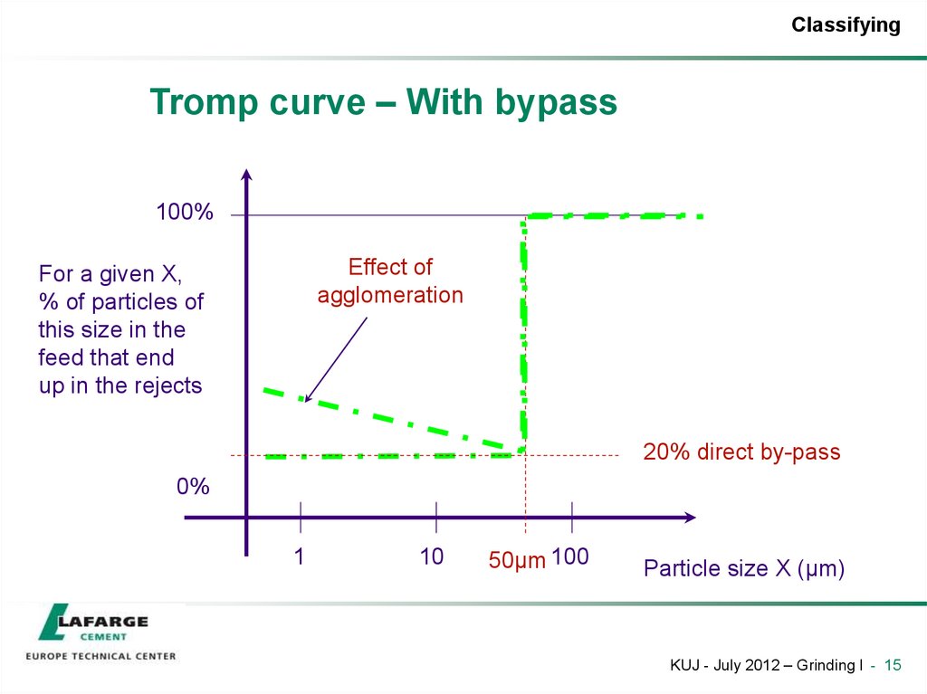
Effect of
agglomeration
For a given X,
% of particles of
this size in the
feed that end
up in the rejects
20% direct by-pass
0%
1
10
50µm 100
Particle size X (µm)
KUJ - July 2012 – Grinding I - 15

16. Imperfection

Classifying
Imperfection
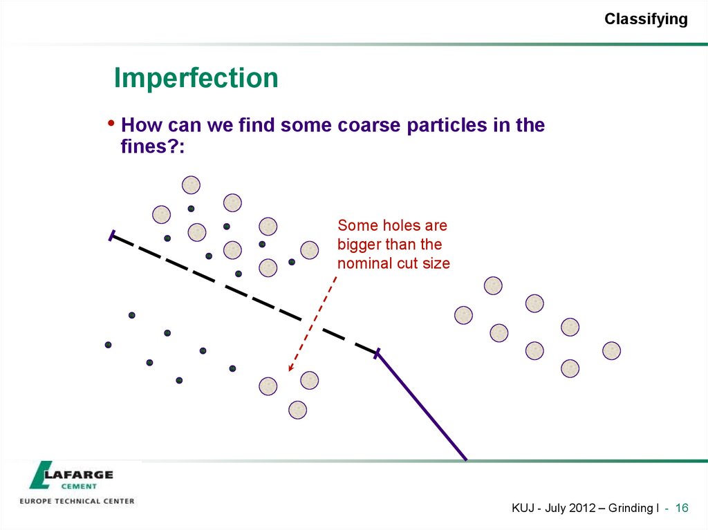
• How can we find some coarse particles in the
fines?:
Some holes are
bigger than the
nominal cut size
KUJ - July 2012 – Grinding I - 16

17. Tromp curve – With imperfection

Classifying
Tromp curve – With imperfection
100%
For a given X,
% of particles of
this size in the
feed that end
up in the rejects
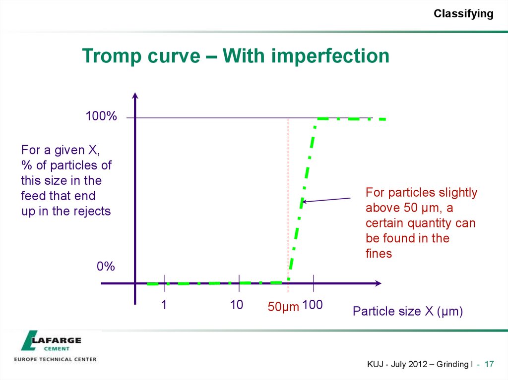
For particles slightly
above 50 µm, a
certain quantity can
be found in the
fines
0%
1
10
50µm 100
Particle size X (µm)
KUJ - July 2012 – Grinding I - 17

18. Tromp curve – General case

Classifying
Tromp curve – General case
100%
90%
80%
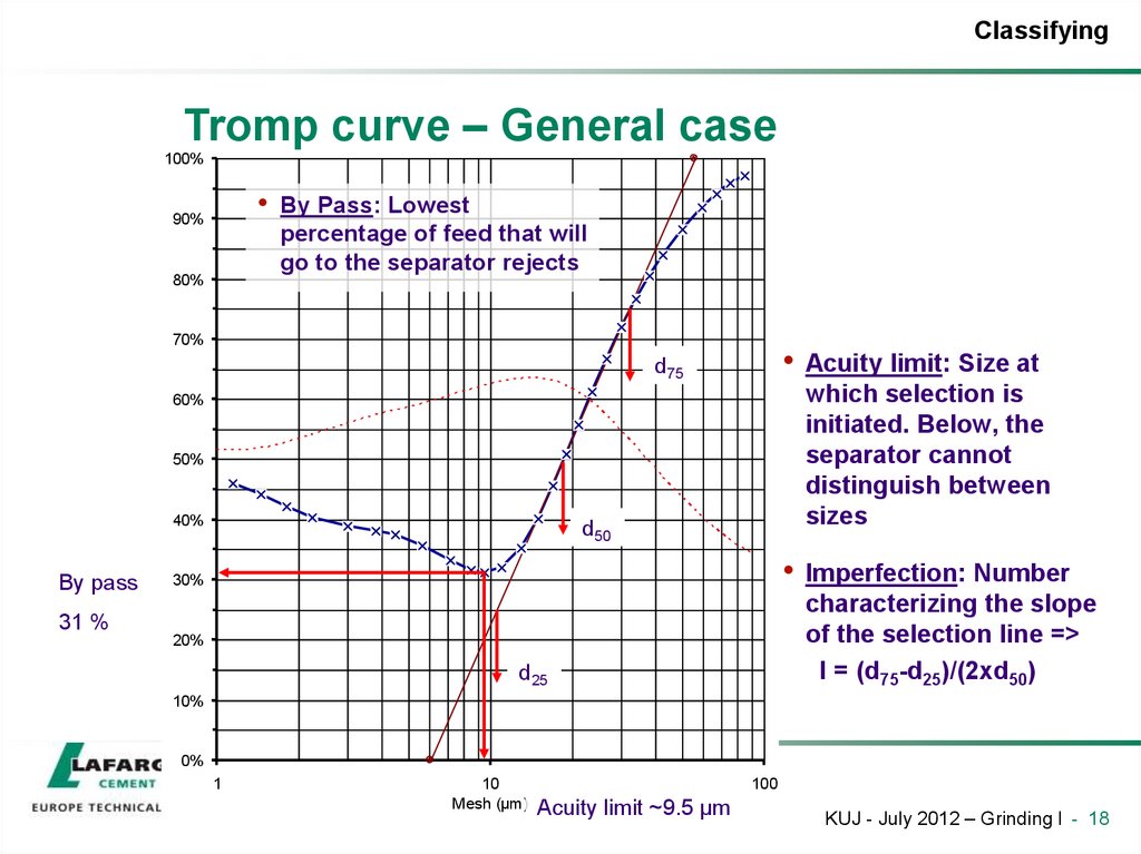
By Pass: Lowest
percentage of feed that will
go to the separator rejects
70%
d75
Acuity limit: Size at
which selection is
initiated. Below, the
separator cannot
distinguish between
sizes
Imperfection: Number
characterizing the slope
of the selection line =>
I = (d75-d25)/(2xd50)
60%
50%
40%
By pass
31 %
d50
30%
20%
d25
10%
0%
1
10
Mesh (µm)
100
Acuity limit ~9.5 µm
KUJ - July 2012 – Grinding I - 18

19. Tromp curve - Interpretation

Classifying
Tromp curve - Interpretation
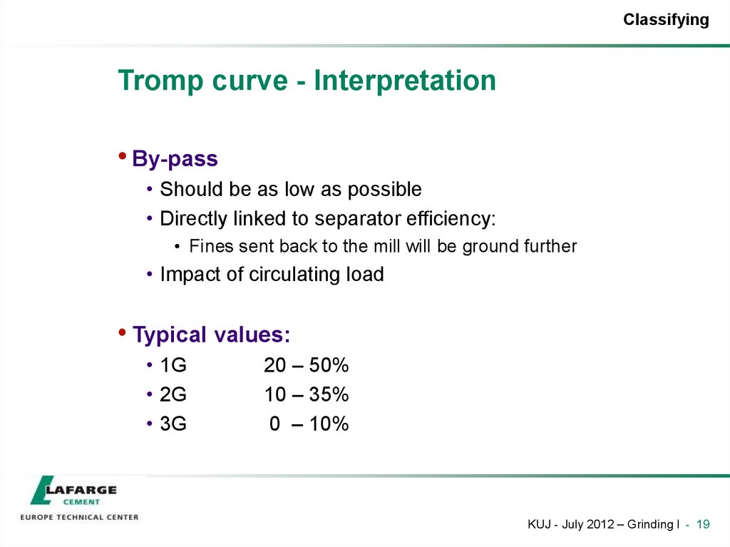
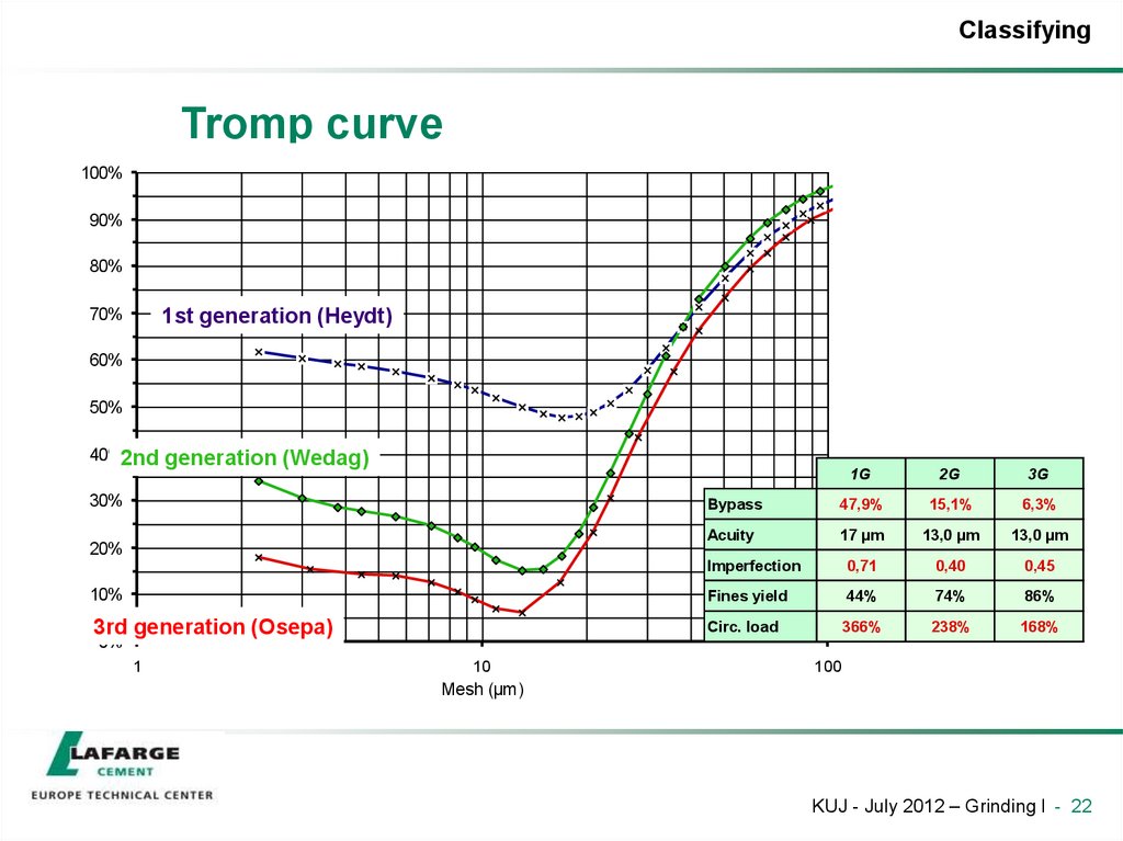
• By-pass
• Should be as low as possible
• Directly linked to separator efficiency:
• Fines sent back to the mill will be ground further
• Impact of circulating load
• Typical values:
• 1G
• 2G
• 3G
20 – 50%
10 – 35%
0 – 10%
KUJ - July 2012 – Grinding I - 19

20. Variation of the By Pass vs CL

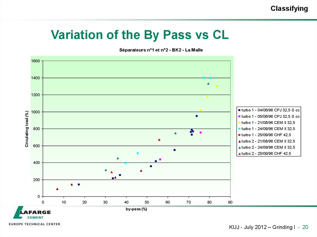
Classifying
Variation of the By Pass vs CL
Séparateurs n°1 et n°2 - BK2 - La Malle
1600
1400
Circulating load (%)
1200
turbo 1 - 04/06/96 CPJ 32,5 S cc
1000
turbo 1 - 05/06/96 CPJ 32,5 S cc
turbo 1 - 21/08/96 CEM II 32,5
800
turbo 1 - 24/09/96 CEM II 32,5
turbo 1 - 25/09/96 CHF 42,5
turbo 2 - 21/08/96 CEM II 32,5
600
turbo 2 - 24/09/96 CEM II 32,5
turbo 2 - 25/09/96 CHF 42,5
400
200
0
0
10
20
30
40
50
60
70
80
90
by-pass (%)
KUJ - July 2012 – Grinding I - 20

21. Tromp curve - Interpretation

Classifying
Tromp curve - Interpretation
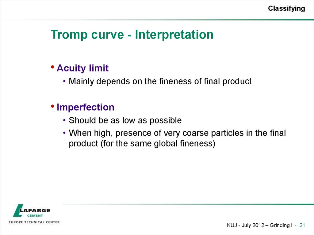
• Acuity limit
• Mainly depends on the fineness of final product
• Imperfection
• Should be as low as possible
• When high, presence of very coarse particles in the final
product (for the same global fineness)
KUJ - July 2012 – Grinding I - 21

22. Tromp curve

Classifying
Tromp curve
100%
90%
80%
1st generation (Heydt)
70%
60%
50%
40%2nd
generation (Wedag)
1G
2G
3G
Bypass
47,9%
15,1%
6,3%
Acuity
17 µm
13,0 µm
13,0 µm
Imperfection
0,71
0,40
0,45
10%
Fines yield
44%
74%
86%
3rd generation (Osepa)
Circ. load
366%
238%
168%
30%
20%
0%
1
10
100
Mesh (µm)
KUJ - July 2012 – Grinding I - 22

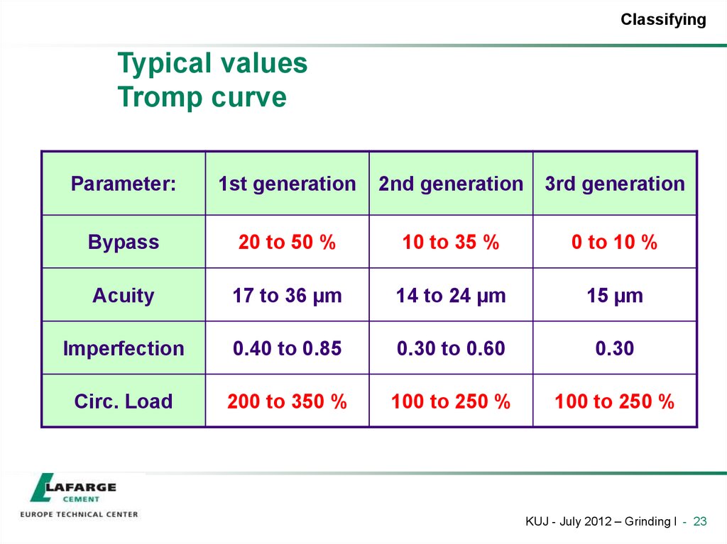
23. Typical values Tromp curve

Classifying
Typical values
Tromp curve
Parameter:
1st generation
2nd generation
3rd generation
Bypass
20 to 50 %
10 to 35 %
0 to 10 %
Acuity
17 to 36 µm
14 to 24 µm
15 µm
Imperfection
0.40 to 0.85
0.30 to 0.60
0.30
Circ. Load
200 to 350 %
100 to 250 %
100 to 250 %
KUJ - July 2012 – Grinding I - 23

24. Building a Tromp curve

Classifying
Building a Tromp curve
• Mass balance
• Knowledge of a physical property of 3 flows gives
access to R/A ratio
• Let’s apply to powders, using laser PSD
KUJ - July 2012 – Grinding I - 24

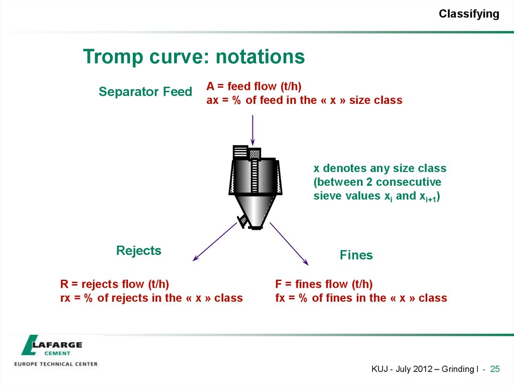
25. Tromp curve: notations

Classifying
Tromp curve: notations
Separator Feed
A = feed flow (t/h)
ax = % of feed in the « x » size class
x denotes any size class
(between 2 consecutive
sieve values xi and xi+1)
Rejects
R = rejects flow (t/h)
rx = % of rejects in the « x » class
Fines
F = fines flow (t/h)
fx = % of fines in the « x » class
KUJ - July 2012 – Grinding I - 25

26. Tromp curves – R/A calculation

Classifying
Tromp curves – R/A calculation
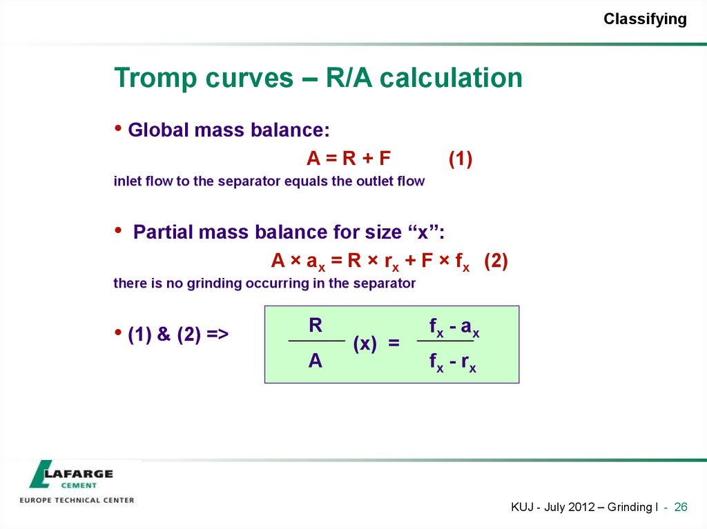
• Global mass balance:
A=R+F
(1)
inlet flow to the separator equals the outlet flow
Partial mass balance for size “x”:
A × ax = R × rx + F × fx (2)
there is no grinding occurring in the separator
• (1) & (2) =>
R
A
(x) =
f x - ax
f x - rx
KUJ - July 2012 – Grinding I - 26

27. 3 point junction (ABC formula)

Classifying
3 point junction (ABC formula)
A, a
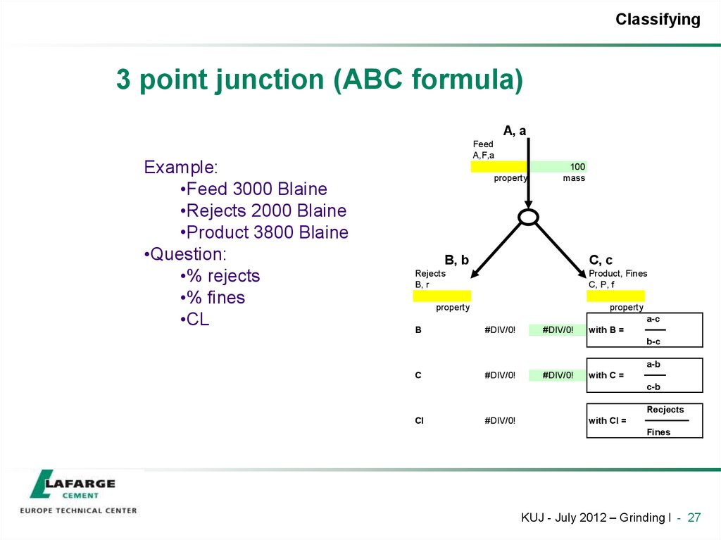
Example:
•Feed 3000 Blaine
•Rejects 2000 Blaine
•Product 3800 Blaine
•Question:
•% rejects
•% fines
•CL
Feed
A,F,a
property
100
mass
B, b
C, c
Rejects
B, r
Product, Fines
C, P, f
property
property
a-c
B
#DIV/0!
#DIV/0!
with B =
b-c
a-b
C
#DIV/0!
#DIV/0!
with C =
c-b
Recjects
Cl
#DIV/0!
with Cl =
Fines
KUJ - July 2012 – Grinding I - 27

28. 3 point junction (ABC formula)

Classifying
3 point junction (ABC formula)
Example:
•Feed 3000 Blaine
•Rejects 2000 Blaine
•Product 3800 Blaine
•Question:
•% rejects
•% fines
•CL
KUJ - July 2012 – Grinding I - 28

29. 3 point junction (ABC formula)

Classifying
3 point junction (ABC formula)
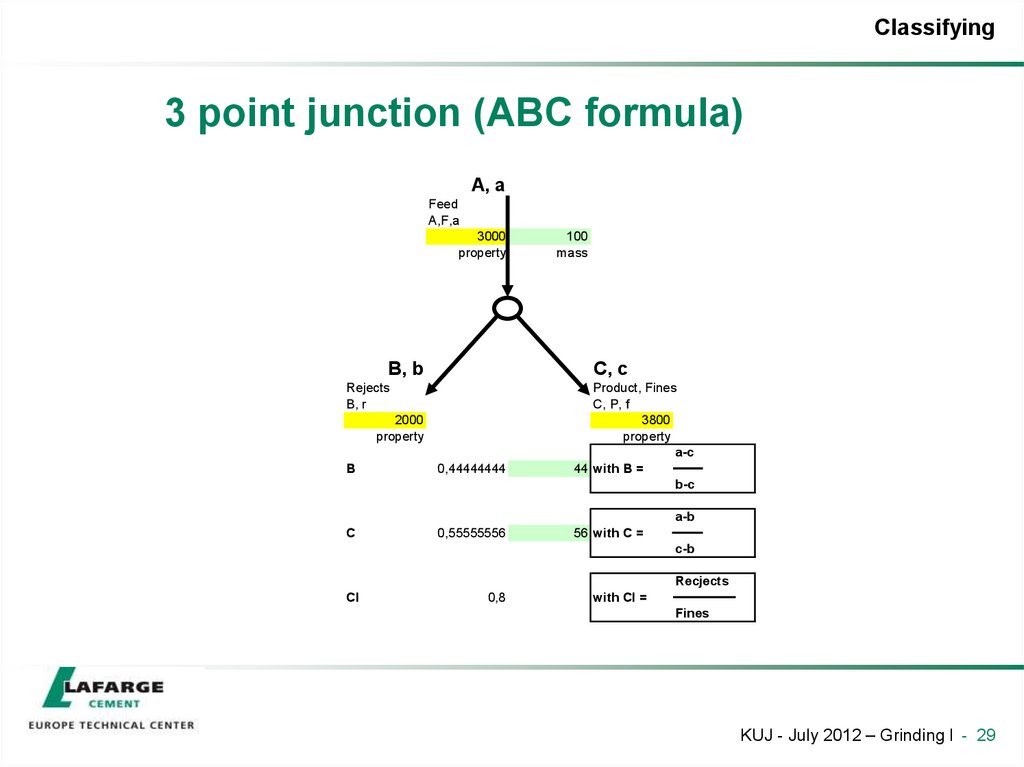
A, a
Feed
A,F,a
3000
property
B, b
100
mass
C, c
Rejects
B, r
2000
property
B
0,44444444
C
0,55555556
Product, Fines
C, P, f
3800
property
a-c
44 with B =
b-c
a-b
56 with C =
c-b
Recjects
Cl
0,8
with Cl =
Fines
KUJ - July 2012 – Grinding I - 29

30. Tromp curves – R/A calculation

Classifying
Tromp curves – R/A calculation
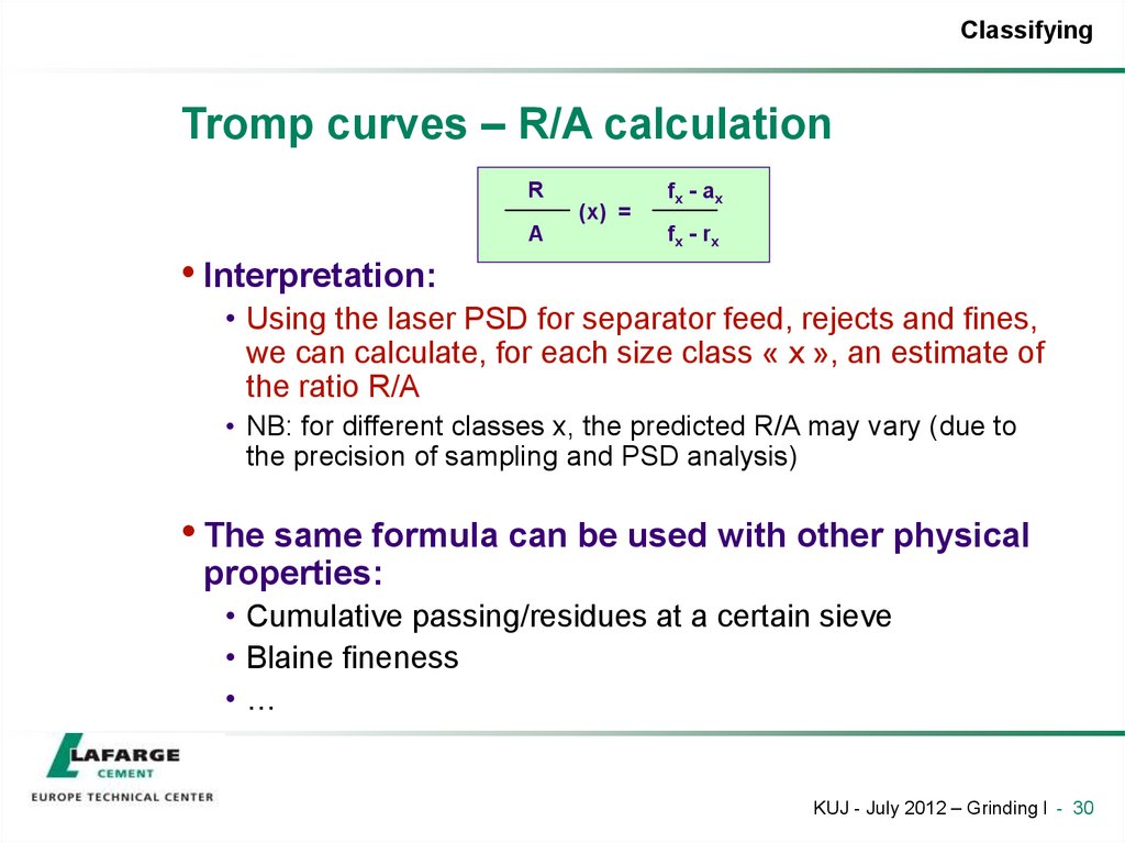
R
(x) =
A
• Interpretation:
fx - ax
fx - r x
• Using the laser PSD for separator feed, rejects and fines,
we can calculate, for each size class « x », an estimate of
the ratio R/A
• NB: for different classes x, the predicted R/A may vary (due to
the precision of sampling and PSD analysis)
• The same formula can be used with other physical
properties:
• Cumulative passing/residues at a certain sieve
• Blaine fineness
•…
KUJ - July 2012 – Grinding I - 30

31. Tromp curves – average R/A

Classifying
Tromp curves – average R/A
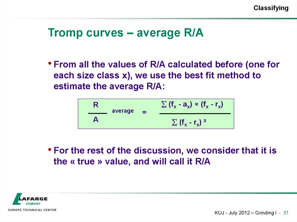
• From all the values of R/A calculated before (one for
each size class x), we use the best fit method to
estimate the average R/A:
R
A
average
(fx - ax) × (fx - rx)
=
(fx - rx) ²
• For the rest of the discussion, we consider that it is
the « true » value, and will call it R/A
KUJ - July 2012 – Grinding I - 31

32. Tromp curves – final calculation

Classifying
Tromp curves – final calculation
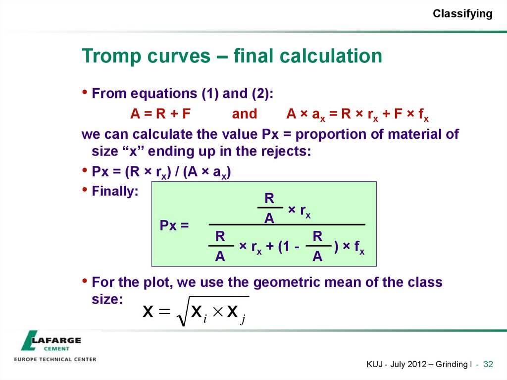
• From equations (1) and (2):
A=R+F
and
A × ax = R × rx + F × fx
we can calculate the value Px = proportion of material of
size “x” ending up in the rejects:
• Px = (R × rx) / (A × ax)
• Finally:
Px =
R
× rx
A
R
R
× rx + (1 ) × fx
A
A
• For the plot, we use the geometric mean of the class
size:
x xi x j
KUJ - July 2012 – Grinding I - 32

33. Tromp curves - How to build?

Classifying
Tromp curves - How to build?
• Evaluate and interprete the tromp curve for a given laser
analysis
KUJ - July 2012 – Grinding I - 33