Reservoir management

1. Reservoir Management

Dan Arnold

2. Learning objectives

1. Provide a formal Management Process
2. Reservoir Management tools
3. Review some examples of Management Strategy
1.
2.
3.
4.
Clastics
Carbonates
Oil
Gas
4. Develop a knowledge of Reservoir Management techniques
and applications
5. Reservoir Management best practice

3.

“The purpose of reservoir management is to
control operations to obtain the maximum
possible economic recovery from a reservoir on
the basis of facts, information and knowledge”
Thakur, 1996 - Chevron

4.

“The marshalling of all appropriate
business, technical and operating
resources to exploit a reservoir optimally
from discovery to abandonment”
“Through-life, ongoing process”
Al-Hussainy and Humphreys, 1996 - Mobil

5.

“There are probably as many different
definitions as there are perceptions of the
process”
“Integrated approach...key consideration...”
“The judicious use of the various means
available to a business to maximise its
benefits/profits from the reservoir”
Egbogah, 1996 - Petronas

6. What is reservoir management? - Summary

Integrated approach:
1. to control operations
2. to maximise benefits/profits (value) from the
reservoir (asset)
3. to obtain the maximum possible economic
recovery from a reservoir

7. A lifetime of reservoir models

8. Forties field – habitat of remaining oil

CHANNEL MARGIN SANDS
ATTIC OIL
ATTIC OIL
TOP RESERVOIR
CHANNEL SANDS
50m
SEAWATER
STRATIGRAPHIC-BYP ASSED OIL
ORIGINAL
OIL-WATER
500m
(from Brand et al., 1996; Scott, 1997)

9. Monetary value of an asset

Recoverable resources (i.e. reserves)
Rate of production
Cost of production
Oil price
Fiscal regime

10. Aim

MAXIMISE
VALUE
• Maximise recovery
• Recovery Technology (speed
up)
• People/Team
• Reservoir Knowledge/analysis
MINIMISE
COST
CAPEX
OPEX
Tax
Depreciation

11. Recovery

Maximise value through…
RECOVERY

12. Recovery Factors

Depends on Geology
Tyler and Finlay, 1991
and Drive Mechanism
Solution gas drive
Gas cap drive
Water drive
Gravity drainage
(after Sills, AAPG Methods 10, 1992)
5-30%
20-40%
35-75%
5-30%

13. Depositional Environment vs Drive Mechanism

• Environment type has
less of an impact on
recovery efficiency
• Primary vs secondary
recovery has a bigger
impact
– Primary recover average
= 20% recovery vs 40%
for secondary recovery
mechanisms
Larue and Friedman, 2005

14. Recover efficiency impact from various reservoir features

Does connectivity influence
recovery?

15. Does connectivity influence recovery?

What is connectivity?
• Sandbody connectivity
– % of sand bodies that are connected to each other
• Reservoir connectivity
– % of sand connected to the wells
– Producer, producer/injector, completions/laterals
• Static and Dynamic connectivity
– How long will it take to produce the connected
volume
– Bypassing?
– Multiple connections?

16. What is connectivity?

Examples of connectivity?
Larue & Hovadik, 2006

17. Examples of connectivity?

Relationship between connectivity and
recovery
Larue & Hovadik, 2006

18. Relationship between connectivity and recovery

Static vs dynamic well connectivity
• Reservoir recoveries
significantly below
percolation prediction of
connected sand bodies
– Static inter-body
connectivity
– Producer sand connectivity
– Producer-injector
connectivity
– Dynamic recovery
efficiency is different
Larue & Hovadik, 2006

19. Static vs dynamic well connectivity

2D Connectivity
Hovadik & Larue, 2010

20. 2D Connectivity

3D percolation connectivity
Hovadik & Larue, 2010

21. 3D percolation connectivity

2D vs 3D connectivity
Larue & Hovadik, 2006

22. 2D vs 3D connectivity

Shifting the S-Curve
Larue & Hovadik, 2006

23. Shifting the S-Curve

Larue & Hovadik, 2006
Shifting the S-Curve Left or Right?
7
1
6
2
8
5
3
4

24. Shifting the S-Curve Left or Right?

Geology that shifts the S-Curve Left
Larue & Hovadik, 2006

25. Geology that shifts the S-Curve Left

Geology that shifts the S-Curve Right
Larue & Hovadik, 2006

26. Geology that shifts the S-Curve Right

Increasing 2D effect (shift to Right)
Larue & Hovadik, 2006

27. Increasing 2D effect (shift to Right)

Volume support and the cascade zone
Larue & Hovadik, 2006

28. Volume support and the cascade zone

Geobody Anisotropy
Hovadik & Larue, 2010

29. Geobody Anisotropy

Sinuosity
Hovadik & Larue, 2010

30. Sinuosity

Grid dimensions – volume support
Hovadik & Larue, 2007/2010

31. Grid dimensions – volume support

Overview
• Increased volume
support increases
width of cascade zone
• Decreasing
“dimensionality” moves
curve to right
• Increasing
dimensionality shifts
curve to the left

32. Overview

Which impact?
Geological Factor
Dimensionality (S-curve shift)
X
Variogram Range
Variogram Anisotropy
X
X
Channel width and thickness
Channel width/thickness ratio
Channel Parallelism
Channel deviation
X
X
X
Continuous mudstone bed %
Local mudstone drapes
Channel clustering
# sealing faults
Fault block size
Fault offset
Fault length
Volume support (dispersion)
X
X
X
X
X
X
X

33. Which impact?

Is connectivity the biggest factor
affecting recovery?
Larue and Friedman, 2005

34. Is connectivity the biggest factor affecting recovery?

30% NTG
Larue and Friedman, 2005

35. 30% NTG

60% NTG
Larue and Friedman, 2005

36. 60% NTG

80% NTG
Larue and Friedman, 2005

37. 80% NTG

Key factors affecting dynamic recovery
• Static connectivity
– SHAPE OF S-CURVE
• Dynamic “addons”
– Tortuosity
– Permeability Heterogeneity
– Inter-well distance
– Fault connectivity
– Fluid

38. Key factors affecting dynamic recovery

Impact of tortuosity
Larue & Hovadik, 2006

39. Impact of tortuosity

Impact of permeability heterogeneity
Larue and Friedman, 2005

40. Impact of permeability heterogeneity

Thief zone impact on recovery
Larue and Friedman, 2005

41. Thief zone impact on recovery

Permeabilty heterogeneity impact
• Small difference between
0D (nugget) and 3D
(variogram) models
• Add trend to increase K at
centre = reduced recovery
• Add drapes and both K
variability and tortuosity
increase
• Compartmentalisation
from mud drapes Further
reduces recovery
Hovadik & Larue, 2010

42. Permeabilty heterogeneity impact

Variogram range and Vdp combined
Hovadik & Larue, 2010

43. Variogram range and Vdp combined

Reservoir Sweep

44. Reservoir Sweep

45. Reservoir Sweep

46. Reservoir Sweep

Impact of mobility ratio
Larue and Friedman, 2005

47. Impact of mobility ratio

Impact of well pattern
Larue and Friedman, 2005

48. Impact of well pattern

Well distance impact on recovery
(dynamic connectivity)
Hovadik & Larue, 2010

49. Well distance impact on recovery (dynamic connectivity)

Does seed really account for
uncertainty?
Larue and Friedman, 2005

50. Does seed really account for uncertainty?

What matters in your reservoir?
Larue and Friedman, 2005

51. What matters in your reservoir?

Extreme edge cases: High NTG + Low
Connectivity
Manzocchi et al, 2007

52. Extreme edge cases: High NTG + Low Connectivity

NTG vs Amalgamation Ratio
• NTG and Amalgamation
ratio do not corellate in
real systems (e.g.
turbidites)
– High NTG vs Low AR
• Object models
Manzocchi et al, 2007

53. NTG vs Amalgamation Ratio

How
willModelling
NTG correlateAswith
AR in an Object
Object
Based
Number of Wells increases.
Simulation may have difficulty in converging
Convergence Problem model?
Illustration of Sequential
Object Based Algorithm (Srivastava 1994)

54. Object Based Modelling Convergence Problem

Geostatistical modelling conditioned
to NTG
• High NTG system has short
continuity of sandbodies
vertically and laterally (<20%)
– Beds terminate early
– Shales laterally extensive
– LOW Amalgamation ratio
• Modelling using Objects
–
–
–
–
(b) sand in shale background
(c) shale in sand background
Neither honour AR of system
Need to model with additional
AR parameter (d)
• Standard Geostats methods
won’t capture the shift to 2D
connectivity due to low AR
Manzocchi et al, 2007

55. Geostatistical modelling conditioned to NTG

Overview of connectivity
NTG
NTG
Impact of
Geology
Geobody size
30% 60%
The threshold at which a
reservoir commonly
starts to connect in 3D
More wells
Increases recovery by
increasing the connected
volume.
The percolation
threshold for a 2D
model.
Lower Mobility
Lowers recovery as oil
viscosity allows for faster
water movement.
Total Recovery
A+B
Geological features can The average recovery
shift curve to left or right, from reservoirs
from 3D to 2D behaviour independent of geology
High Vdp
High permeability
heterogeneity greatly
reduces recovery.
NTG >35%
Has little impact on
recovery factor above
the percolation threshold
Is the sum of the
connected volume (A)
and recovery factor (B)
Seed
Has little impact on
recovery globally, only
local variations for wells.

56. Overview of connectivity

Maximise value through…
IMPROVED RECOVERY

57. Improved Recovery

Recovery Factors
Depends on Geology
Tyler and Finlay, 1991
and Drive Mechanism
Solution gas drive
Gas cap drive
Water drive
Gravity drainage
(after Sills, AAPG Methods 10, 1992)
5-30%
20-40%
35-75%
5-30%

58. Recovery Factors

Improved Recover Factors
Tyler and Finlay, 1991

59. Improved Recover Factors

What can we adjust to improve
recovery?

60. What can we adjust to improve recovery?

Demand growth
Petroleum Industry Drivers
120
Exploration success
Million BOPD
100
80
60
New field
developments
40
20
0
1980
1990
2000
History
Production improvement
New field development
Evaluation of history,
IHS data base
2010
2020
Natural decline
IOR
Exploration
Natural decline “as is”
2030
Reserve growth; IOR
and EOR
Production efficiency
From Meling, 2004

61.

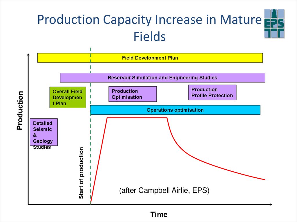
Production Capacity Increase in Mature
Fields
Field Development Plan
Reservoir Simulation and Engineering Studies
Overall Field
Developmen
t Plan
Production
Profile Protection
Production
Optimisation
Detailed
Seismic
&
Geology
Studies
Start of production
Operations optimisation
(after Campbell Airlie, EPS)
Time

62.

Production Capacity Increase in Mature
Fields
Field Development Plan
Reservoir Simulation and Engineering Studies
Overall Field
Developmen
t Plan
Production
Profile Protection
Production
Optimisation
Detailed
Seismic
&
Geology
Studies
Start of production
Operations optimisation
Mature Field
Management
(after Campbell Airlie, EPS)
Time

63.

Example of….
INFILL DRILLING

64. Infill drilling

Field Oil Production Rate
A typical example of the north sea
40
Wells to
Maintain Plateau
+50
Wells to
Target Unswept Oil
and
Extend Field Life
Time

65. A typical example of the north sea

RM Example 1
• Strategy for Statfjord
– Aadland et al., 1994
High well activity
Horizontal wells
Reservoir simulation
Proactive
Investment for future

66. RM Example 1

Statfjord Field - cross section
BRENT
GOC
200m
OWC
GOC
OWC
500m
STATFJORD

67. Statfjord Field - cross section

Statfjord Field - initial production
plan
BRENT
200m
STATFJORD
Oil production
Gas injection
Water injection
500m

68. Statfjord Field - initial production plan

Statfjord Field - Remaining oil
BRENT
Attic oil
Stratigraphic
compartment
s
Structural
compartment
s
200m
Rim oil
STATFJORD
Remaining oil locations
500m

69. Statfjord Field - Remaining oil

Statfjord Field - New opportunities
BRENT
New completions
High angle wells
Infill wells
200m
Horizontal wells
Extended reach
drilling (ERD)
Remaining oil locations
STATFJORD
500m

70. Statfjord Field - New opportunities

Example: Yibal Field, Oman
• Strategy for Yibal Field, Oman
• Horizontal wells
• Bypassed oil in a Carbonate

71. Example: Yibal Field, Oman

Upper Thief Zone:
• Dual pore system
• Uncertain continuity
• Uncertain keff
Modelling Characteristics and
Sensitivities
Lower Thief Layer:
• Dual pore system
• Uncertain continuity
• Uncertain keff
Upper Shuaiba Matrix:
• Single pore system
• Uncertain Kv/Kh ratio
• Uncertain So,r
• Uncertain keff
Original OWC
Tight Streak:
• Baffle to flow
• Uncertain keff
• Uncertain continuity
Fault and Fracture Network:
• Uncertain and varying
conductivity
• Uncertain density
• Uncertain keff

72. Modelling Characteristics and Sensitivities

Yibal Field Development History
1979
Depletion and “phase” injection
1994
Onset of horizontal drilling
1985
Aquifer injection
2002
High density horizontal infill
(from Mijnsen et al, 2005)

73. Yibal Field Development History

YIBAL FIELD: Water - Oil Rate vs RF
9
8
7
WOR (frac)
6
5
4
3
2
1
0
0
0.1
0.2
0.3
0.4
Recovery Factor (frac)
01/81
Phase
01/88
Aquifer Injection
01/94
09/98
Horizontals
0.5

74. YIBAL FIELD: Water - Oil Rate vs RF

FROM CHAPTER 1
Impact of well placement
fluvial study
N
SW
NE
compartmentalisation
of pay facies
Seifert et al., 1996

75. Impact of well placement fluvial study

FROM CHAPTER 1
Impact of well placement
fluvial study
• find orientation of well trajectory most likely to
– contain > aeolian GU proportions
• maximise productivity
– intersect > number of aeolian bodies
• maximise drainage
• assess the likelihood of wells in this orientation intersecting
high proportions of aeolian GUs
Seifert et al., 1996

76. Impact of well placement fluvial study

FROM CHAPTER 1
Impact of well placement
results
aeolian
bodies
intersected
aeolian GU
proportions
horizontal wells
cumulative
aeolian
intersected
# of times in
top 3 rank
inclined wells
well length (ft)
Seifert et al., 1996

77. Impact of well placement results

RM Example 3: Heather Field
Compartmentalisation and Variable Recovery
Tarbert & Ness show overpressure as a
result of continued injection from H05
3500
4500
5500
6500
7500
-10675
E Block Average ( 39% )
Upper Brent
0%
-10700
10%
20%
30%
40%
50%
40%
50%
Tarbert
Up. Ness
Low. Ness
-10725
Etive
Rannoch
-10750
Up. Broom
Low. Broom
-10775
Crest
Lower Brent
-10800
-10825
C Block Average ( 18% )
c. datum pressure
0%
10%
20%
-10850
Tarbert
Up. Ness
-10875
Low. Ness
Etive
Rannoch
-10900
Up. Broom
Low. Broom
-10925
Flank
30%

78. RM Example 3: Heather Field Compartmentalisation and Variable Recovery

Infill Drilling – Heather Field
1 Km
Fault Y
Fault X
2/5 Block
Boundary
H-44 Injector
TARGET TD
Intersection with Fault X
H-62 Well Track
Brent Entry
Fault compartmentalisation

79. Infill Drilling – Heather Field

Example of….
FRACCING

80. fraccing

Example: Leman Field
• Strategy for Leman Field
– Mijnsson and Maskall 1994
• Proactive hunt for gas
• Horizontal wells
– Parallel to palaeowind
Main Wind Direction
10m
Interdune
Dune
Well
0
1 km
Dune
K
K
= 2 - 12
K
K
Interdune
= 20 - 75
K = Permeability parallel to lamination
• Only part of the story
K = Permeability perpendicular to laminate
= Permeability of dune sands
= Permeability of interdune sands
Indicates main inflow direction
(Weber, 1987)

81. Example: Leman Field

Typical Rotliegend reservoir section
SUBSEISMIC
FAULTS
TOP RESERVOIR
WEISLIEGENDES
200m
ORIGINAL
GAS
WATER
CONTACT
500m

82. Typical Rotliegend reservoir section

Stratigraphic/structurally
bypassed gas
SUBSEISMIC
FAULTS
TOP RESERVOIR
WEISLIEGENDES
200m
ORIGINAL
GAS
WATER
CONTACT
Bypassed gas
500m

83. Typical Rotliegend reservoir section

Stratigraphic/structurally
bypassed gas
SUBSEISMIC
FAULTS
TOP RESERVOIR
WEISLIEGENDES
200m
ORIGINAL
GAS
WATER
CONTACT
Horizontal well/multilateral opportunities
500m
Fraccing

84. Typical Rotliegend reservoir section

Example of….
EOR (WAG)

85. EOR (WAG)

IOR: New opportunities with CO2
mbd
80
Initial Waterflood
60
Main CO2 flood
40
ROZ CO2 flood
20
0
1970
1990
2010
2030

86. IOR: New opportunities with CO2

Example: Magnus Field
Production & Injection History
Magnus Field Production (and Gas Injection) History
200
Water Rate
Gas Injection
150
100
Commence gas
injection for EOR
Commence water
injection
50
Additional
well slots
2010
2009
2008
2007
2006
2005
2004
2003
2002
2001
2000
1999
1998
1997
1996
1995
1994
1993
1992
1991
1990
1989
1988
1987
1986
1985
1984
0
1983
Production and Injection Rates mboed
Oil Rate
Moulds et al, 2010, SPE 134953

87. Example: Magnus Field Production & Injection History

Improved oil recovery from EOR over
waterflood
Moulds et al, 2010, SPE 134953

88. Improved oil recovery from EOR over waterflood

The Future – New Wells
• Magnus Extension Project
– 4 new slots, slot splitter technology enables 2 wells from each slot
• 13 well drilling programme under-way
7
4
5
6
6
1
10
10
8a
8
8b
13
11
11
2
M56Z:E8
M57Z:E7
M 57Z:E7 North-West
M agnus producer
Magnus Platform Oil Rate (mstb/d)
9
3
M 56Z:E8 Southern panel EOR producer
3
2
12
12
1
M58Z:E3
M59Z:E4
M 58Z:E3 LKCF reservoir producer
30
4
M 59Z:E4 North-West M agnus injector
5
M 60:A6
Southern panel EOR producer
future target
20
10
0
Sep-08
Jan-09
May-09
Sep-09
Jan-10
Moulds et al, 2010, SPE 134953

89. The Future – New Wells

Target: Magnus Field
Oil Remaining after waterflood
M 56Z:E8
Southern panel
producer
M 60:A6
Southern panel
producer
M 58Z:E3
M SM sands
show n here
although w ell
drilled and
completed as
an LKCF
producer
EOR oil target: updip attic target and unswept oil under shales
Moulds et al, 2010, SPE 134953

90. Target: Magnus Field Oil Remaining after waterflood

Maximise value through…
PEOPLE/TEAMS

91. People/teams

Synergy
Output of a synergistic team is larger than the
sum of the output of individuals….
Geol
+ Geoph
+
=
Eng
=
Output
Output
Sneider, 2000

92. Synergy

• Is not:
– Geoengineering
– Any thing about multi-discipline work
– Anything to do with Energy
• Synergy
– Sum of the parts are greater than they are
individually

93. Synergy

REM is like Systems thinking
• System of interdependent
processes
• Model Complexity of system
rather than simplify
• People in parts of system need
to work together and
communicate
• Geology, petrophysics,
geophysics, reservoir
engineering, drilling,
petroleum engineering,
upstream/downstream,
environment, local
populations, governments…..
The list goes on

94. REM is like Systems thinking

Field Management Plan (UK DTI)
• Reservoir Management Strategy
• - detailing the principles and objectives that the operator will hold when
making field management decisions and conducting field operations
• Reservoir Monitoring Plan
• - describing the data gathering and analysis proposed to resolve existing
uncertainties and understand dynamic performance during development
drilling and subsequent production
Owen, 1998

95. Field Management Plan (UK DTI)

RM Strategy
Developing
Implementing
Monitoring
Evaluating
• DIME - Satter and Thakur, 1994

96. RM Strategy

Increase costs through…
WATER MANAGEMENT

97. Water management

Reservoir Management Issues (1)
(From Arnold
et al., 2004)
a- Mechanical leaks: b - Behind Casing flow
c - Oil-water contact: d – High perm zones

98. Reservoir Management Issues (1)

Reservoir Management Issues (2)
e- Fractures: f – Fractures to water
g - Coning: h – Areal sweep
i – Gravity segregation
j – High perm with crossflow

99. Reservoir Management Issues (2)

Example of….
WATER SHUTOFF

100. Water shutoff

Yibal Field Development History
1979
Depletion and “phase” injection
1994
Onset of horizontal drilling
1985
Aquifer injection
2002
High density horizontal infill
(from Mijnsen et al, 2005)

101. Yibal Field Development History

YIBAL FIELD: Water - Oil Rate vs RF
9
8
7
WOR (frac)
6
5
4
3
2
1
0
0
0.1
0.2
0.3
0.4
Recovery Factor (frac)
01/81
Phase
01/88
Aquifer Injection
01/94
09/98
Horizontals
0.5

102. YIBAL FIELD: Water - Oil Rate vs RF

Brent Field Reservoir monitoring
A
B
C
B
A
B
A
ETIVE
WELLS
THIEF ZONE
PLT
PAY
81 85
ORIG. NOW
PERF 81
4
RANNOCH
CEMENT 85
3
PERF 89
2
BROOM
RFT 85
(corrected to datum)
PERF 87
OWC
1
OIL
1975
1980
OIL-PRODUCING
THIEF ZONE
WATER
1985
WATER INJECTION
1990
GAS INJECTION
(Bryant and Livera, 1991)

103. Brent Field Reservoir monitoring

WELLS
A
B
C
B
A
B
1. Initial Conditions
A
ETIVE
Ness Formation
THIEF ZONE
PLT
PAY
81 85
ORIG. NOW
PERF 81
4
RANNOCH
CEMENT 85
3
PERF 89
2
BROOM
RFT 85
(corrected to datum)
PERF 87
OWC
1
OIL
1975
1980
OIL-PRODUCING
THIEF ZONE
WATER
1985
WATER INJECTION
1990
GAS INJECTION
(Bryant and Livera, 1991)

104. Brent Field Reservoir monitoring

Water Shut-off
WELLS
A
B
C
B
A
B
A
1. 1987 Conditions
ETIVE
Ness Formation
THIEF ZONE
PLT
PAY
81 85
ORIG. NOW
PERF 81
RANNOCH
4
CEMENT 85
3
PERF 89
BROOM
2
OIL
THIEF ZONE
WATER
RFT 85
(corrected to datum)
PERF 87
OWC
1
1975
1980
OIL-PRODUCING
1985
WATER INJECTION
1990
GAS INJECTION
Profile
Modification
(Bryant and Livera, 1991)
New
Perforations

105. Brent Field Reservoir monitoring

Increase costs through…
SCALE MANAGEMENT

106. Scale management

Decline in Magnus production
Moulds et al, 2010, SPE 134953

107. Decline in Magnus production

Examples - Flow Restriction

108. Examples - Flow Restriction

Examples - Facilities
separator scaled up
and after
cleaning

109. Examples - Facilities

Water chemistry history match
154471 • Use of Water Chemistry Data in History Matching of a Reservoir Model • Dan Arnold

110. Water chemistry history match

Probabilistic predictions of scaling in
wells
Spatial Probability Maps
Tracer concentration
Well Forecasts
Time
154471 • Use of Water Chemistry Data in History Matching of a Reservoir Model • Dan Arnold

111. Probabilistic predictions of scaling in wells

Predicting Seawater fraction in
produced water
(Vasquez et al., 2013)

112. Predicting Seawater fraction in produced water

Probability maps of seawater fraction
P10
P50
P90

113. Probability maps of seawater fraction

Results
• Optimization w/o accounting scale risk
2
2
SeaWater Fraction
OilSaturation Layer 2

114. Results

• Optimization accounting scale risk
5
4
SeaWater Fraction
OilSaturation Layer 4
OilSaturation Layer 1

115. Results

Layer open/shut
• w/o accounting scale risk
• accounting scale risk
1
2
3
4
5
Oil Saturation
0
1

116. Results

Impact in the value through…
VALUE OF YOUR OIL

117. Value of your Oil

Two key things you don’t know
• How much oil you can
extract
– Reservoir uncertainty
– Variations from different
development plans
– Ownership
• How much your oil is
worth
–
–
–
–
Oil price
Lifting costs
CAPEX
Taxation/Royalty

118. Two key things you don’t know

All oil is not created equally priced...

119. All oil is not created equally priced...

Time value of money
“how much money would have to be invested currently, at a
given rate of return, to yield the cash flow in future.”
where
•DPV is the discounted present value of the future cash flow (FV), or FV adjusted for the delay in receipt;
•FV is the nominal value of a cash flow amount in a future period;
•i is the interest rate or discount rate, which reflects the cost of tying up capital and may also allow for the risk
that the payment may not be received in full;[1]
•n is the time in years before the future cash flow occurs

120. Time value of money

Value of money decreases overtime
(NPV)
From wikipedia

121. Value of money decreases overtime (NPV)

Compare value of companies
• Oil = 5,817 million
barrels
• Gas = 24,948 billion
cubic feet
• 1.75 million BOE per
day
• Oil = 2,234 million
barrels
• Gas = 3,810 billion cubic
feet
• 753,000 BOE per day
production
$6.8 billion net income
$4.6 billion net income
Market cap = 83.28bn
Market cap = 77.63bn

122. Compare value of companies

Compare strategy of companies
• Offshore, deep water,
complex fields
• Ultra high production
(60,000 bpd + per well)
• High well costs ($150
million + per well)
• Ultra high CAPEX
• Long development cycles
(6 years)
• Onshore, EOR, easy
access, shallow
• Low production (5001000bpd)
• Low CAPEX/high OPEX
($10/bbl)
• Low well cost ($2-4
million)
• Fast turn around times
on wells (less than 1
year)

123. Compare strategy of companies

Lifting cost of oil (worldwide)

124. Lifting cost of oil (worldwide)

Angus field NS
Why the stop in
production for 10
years?

125. Angus field NS

Aim
MAXIMISE
VALUE
Maximise recovery
Speed up recovery
People/Team
Reservoir Knowledge/analysis
Recovery Technology
MINIMISE
COST
CAPEX
OPEX
Tax
Depreciation

126. Aim

MAXIMISE
VALUE
Maximise recovery
Speed up recovery
People/Team
Reservoir Knowledge/analysis
Recovery Technology
MINIMISE
COST
CAPEX
OPEX
Tax
Depreciation

127. Aim

Value and Risk: Expected Return
• Expected loss/gain for an event is sum of
probabilities*loss/gains for each event
E(R) = 0.5 × £10 + 0.25 × £20 + 0.25 × (-£10) = £7.5
Loss/Gain
Probability
£10
50%
£20
25%
-£10
25%

128. Value and Risk: Expected Return

Decision tree analysis

129. Decision tree analysis

Discretisation of PDFs
• Convert continuous values into discrete to use
in decision tree
• Several methods, such as:
– Swanson’s rule (P10/50/90 = 30%/40%/30%)
– Pearson Tukey (P10/50/90 = 18.5%/63%/18.5%)
– McNamee & Celona Shortcut (25%/50%/25%)
P10 P50
P90

130. Discretisation of PDFs

Maximise value through…
RESERVOIR DEVELOPMENT
OPTIMISATION

131. Reservoir development optimisation

What do we mean by optimisation
• Process of improving something
– to find the best compromise among several often
conflicting requirements
– Constantly updating/improving process vs defined
decision points
– Maximising value, minimising risk/impact,
lowering cost
– Integrated solution in complex systems

132. What do we mean by optimisation

Optimisation example
Model 1
Model 2

133. Optimisation example

Optimisation often involves trade-offs
MAXIMISE
VALUE
Maximise recovery
Speed up recovery
People/Team
Reservoir Knowledge/analysis
Recovery Technology
MINIMISE
COST
CAPEX
OPEX
Tax
Depreciation

134. Optimisation often involves trade-offs

Automated optimisation
• A set of algorithms available
that can automate the
optimisation process
• Define problem as a set of
optimisation parameters in the
model
• Algorithm adjusts these
automatically to find “optimal
solutions”
• Algorithm steps iteratively,
converging on the “best
answer”
• Multiple competing criteria
means a trade-off in the
optimal solution

135. Automated optimisation

Optimization Algorithm
• Particle Swarm Optimization (PSO)
objective
min
p2
p1
• Particles move based on their own
experience and that of the swarm
L. Mohamed (2010)
max

136. Optimization Algorithm

How many wells?
• Vary well status and well locations
Model 2
Model 1

137. How many wells?

Real life trade-off in optimisation
• Vary injection well rates and locations of wells
– Well rates in [0,15] MBD

138. Real life trade-off in optimisation

MSc students vs an algorithm?
77 models
10%
Original MSc development plan
(4 injectors, 4 producers)
Current Scapa production
55%

139. MSc students vs an algorithm?

Optimization of Infill Well Locations
Trade-off:
~1.2 bbls long term
1 bbl short term
MOBOA – Multi-Objective Bayesian Optimisation Algorithm

140. Optimization of Infill Well Locations

In review
Creating value from of our asset
Ongoing, Life-of-field process
Risk in decisions from uncertainty in the field
We can increase value or decrease costs
Geology and engineering are both important
identifying the best development plan