


 economics
Similar presentations:


")

10 principles of economics
1.
MACROECONOMICS10 PRINCIPLES OF
ECONOMICS
Zharova Liubov
Zharova_l@ua.fm
2.
ECONOMY…. . . The word economy comes from a Greek word
for “one who manages a household.”
3.
PRINCIPLES OF ECONOMICSA household and an economy face many
decisions:
Who will work?
● What goods and how many of them should be
produced?
● What resources should be used in production?
● At what price should the goods be sold?
4.
PRINCIPLES OF ECONOMICSSociety and Scarce Resources:
The management of society’s resources is important
because resources are scarce.
● Scarcity. . . means that society has limited resources
and therefore cannot produce all the goods and
services people wish to have.
5.
ECONOMICSEconomics is the study of how society manages its
scarce resources.
The branch of knowledge concerned with the
production, consumption and transfer of wealth
6.
10 PRINCIPLES OF ECONOMICSHow people make decisions.
1. People face tradeoffs.
2. The cost of something is what you give up to get
it.
3. Rational people think at the margin.
4. People respond to incentives.
7.
10 PRINCIPLES OF ECONOMICSHow people interact with each other.
5. Trade can make everyone better off.
6. Markets are usually a good way to organize
economic activity.
7. Governments can sometimes improve economic
outcomes.
8.
10 PRINCIPLES OF ECONOMICSThe forces and trends that affect how the
economy as a whole works.
8. The standard of living depends on a country’s
production.
9. Prices rise when the government prints too
much money.
10. Society faces a short-run tradeoff between
inflation and unemployment.
9.
PRINCIPLE #1: PEOPLE FACE TRADEOFFSTrade off is a situation that involves losing one
quality or aspect of something in return for
gaining another quality or aspect
“There is no such thing as a free lunch!”
10.
PRINCIPLE #1: PEOPLE FACE TRADEOFFSTo get one thing, we usually have to give up
another thing.
Food v. clothing
● Leisure time v. work
● Efficiency v. equity
Making decisions requires trading off one
goal against another
11.
PRINCIPLE #1: PEOPLE FACE TRADEOFFSEfficiency v. Equity
Efficiency means society gets the most that it can from
its scarce resources.
● Equity means the benefits of those resources are
distributed fairly among the members of society.
12.
PRINCIPLE #2: THE COST OF SOMETHINGIS WHAT YOU GIVE UP TO GET IT
Decisions require comparing costs and benefits of
alternatives.
Whether to go to college or to work?
● Whether to study or go out on a date?
● Whether to go to class or sleep in?
The opportunity cost of an item is what you give
up to obtain that item.
13.
PRINCIPLE #2: THE COST OF SOMETHINGIS WHAT YOU GIVE UP TO GET IT
Cricketing god Sachin
Tendulkar decided to quit
his education in order to
play professional cricket for
his country.
LA Laker basketball star
Kobe Bryant chose to skip
college and go straight from
high school to the pros where
he has earned millions of
dollars.
14.
PRINCIPLE #3: RATIONAL PEOPLE THINKAT THE MARGIN
Rational people people who systematically and
purposefully do the best they can to achieve their
objectives
Marginal changes are small, incremental
adjustments to an existing plan of action.
People make decisions by comparing costs
and benefits at the margin
15.
PRINCIPLE #4: PEOPLE RESPOND TOINCENTIVES
Incentives – something that induces a person to
act
Marginal changes in costs or benefits motivate
people to respond.
The decision to choose one alternative over
another occurs when that alternative’s marginal
benefits exceed its marginal costs!
16.
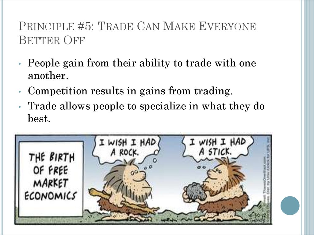
PRINCIPLE #5: TRADE CAN MAKE EVERYONEBETTER OFF
People gain from their ability to trade with one
another.
Competition results in gains from trading.
Trade allows people to specialize in what they do
best.
17.
PRINCIPLE #6: MARKETS ARE USUALLY AGOOD WAY TO ORGANIZE ECONOMIC ACTIVITY
A market economy is an economy that allocates
resources through the decentralized decisions of
many firms and households as they interact in
markets for goods and services.
Households decide what to buy and who to work for.
● Firms decide who to hire and what to produce
18.
PRINCIPLE #6: MARKETS ARE USUALLY AGOOD WAY TO ORGANIZE ECONOMIC ACTIVITY
Adam Smith made the observation that
households and firms interacting in markets act
as if guided by an “invisible hand.”
Because households and firms look at prices when
deciding what to buy and sell, they unknowingly take
into account the social costs of their actions.
● As a result, prices guide decision makers to reach
outcomes that tend to maximize the welfare of society
as a whole.
19.
PRINCIPLE #7: GOVERNMENTS CANSOMETIMES IMPROVE MARKET OUTCOMES
Market failure occurs when the market fails to
allocate resources efficiently.
When the market fails (breaks down) government
can intervene to promote efficiency and equity
20.
PRINCIPLE #7: GOVERNMENTS CANSOMETIMES IMPROVE MARKET OUTCOMES
Market failure may be caused by
● an externality, which is the impact of one
person or firm’s actions on the well-being of a
bystander.
● market power, which is the ability of a single
person or firm to unduly influence market
prices.
21.
PRINCIPLE #8: THE STANDARD OF LIVINGDEPENDS ON A COUNTRY’S PRODUCTION
Standard of living may be measured in different
ways:
● By comparing personal incomes.
● By comparing the total market value of a
nation’s production.
22.
PRINCIPLE #8: THE STANDARD OF LIVINGDEPENDS ON A COUNTRY’S PRODUCTION
Almost all variations in living standards are
explained by differences in countries’
productivities.
Productivity is the amount of goods and services
produced from each hour of a worker’s time.
Standard of living may be measured in different
ways:
By comparing personal incomes.
● By comparing the total market value of a nation’s
production.
23.
PRINCIPLE #9: PRICES RISE WHEN THEGOVERNMENT PRINTS TOO MUCH MONEY
Inflation is an increase in the overall level of
prices in the economy.
One cause of inflation is the growth in the quantity of
money.
● When the government creates large quantities of
money, the value of the money falls.
24.
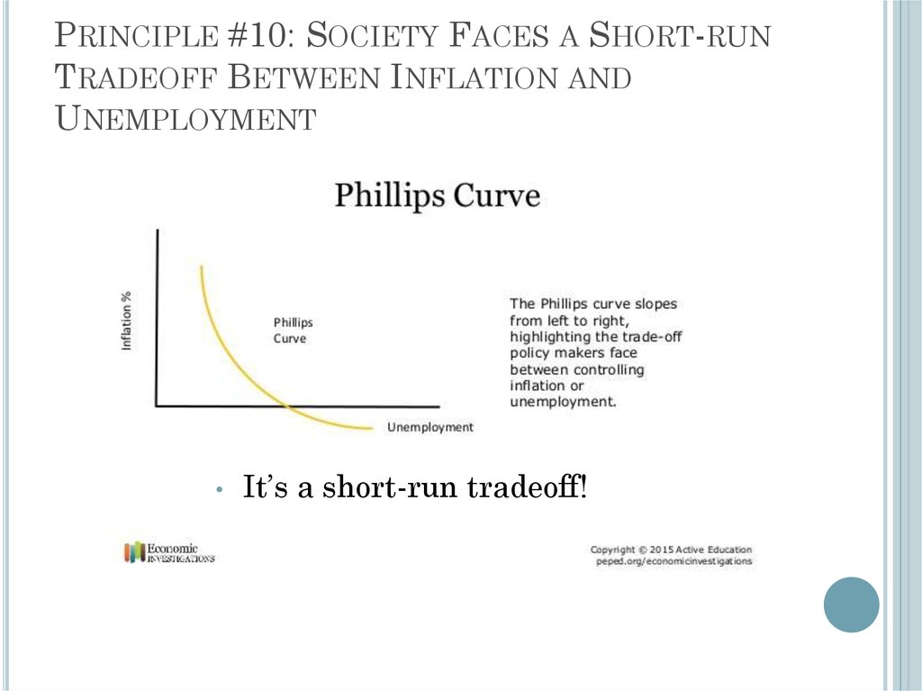
PRINCIPLE #10: SOCIETY FACES A SHORT-RUNTRADEOFF BETWEEN INFLATION AND
UNEMPLOYMENT
It’s a short-run tradeoff!
25.
SUMMARYWhen individuals make decisions, they face
tradeoffs among alternative goals.
The cost of any action is measured in terms of
foregone opportunities.
Rational people make decisions by comparing
marginal costs and marginal benefits.
People change their behavior in response to the
incentives they face.
26.
SUMMARYTrade can be mutually beneficial.
Markets are usually a good way of coordinating
trade among people.
Government can potentially improve market
outcomes if there is some market failure or if the
market outcome is inequitable
27.
SUMMARYProductivity is the ultimate source of living
standards.
Money growth is the ultimate source of inflation.
Society faces a short-run tradeoff between
inflation and unemployment.
28.
MACROECONOMICSINTRODUCTION TO
MACROECONOMICS
Zharova Liubov
Zharova_l@ua.fm
29.
INTROindividual decision-making Microeconomics
examines the behavior of units—business firms
and households.
Macroeconomics deals with the economy as a
whole; it examines the behavior of economic
aggregates such as aggregate income,
consumption, investment, and the overall level of
prices.
Aggregate behavior refers to the behavior of all
households and firms together.
30.
INTROWhen we study the consumption behaviour or
equilibrium of a consumer; the production
pattern & equilibrium of a firm, the entire
analysis is ‘micro’ in nature……because
we study a UNIT and not the SYSTEM in which
it is operating
31.
INTROMacroeconomists often reflect on the
microeconomic principles underlying
macroeconomic analysis, or the microeconomic
foundations of macroeconomics
32.
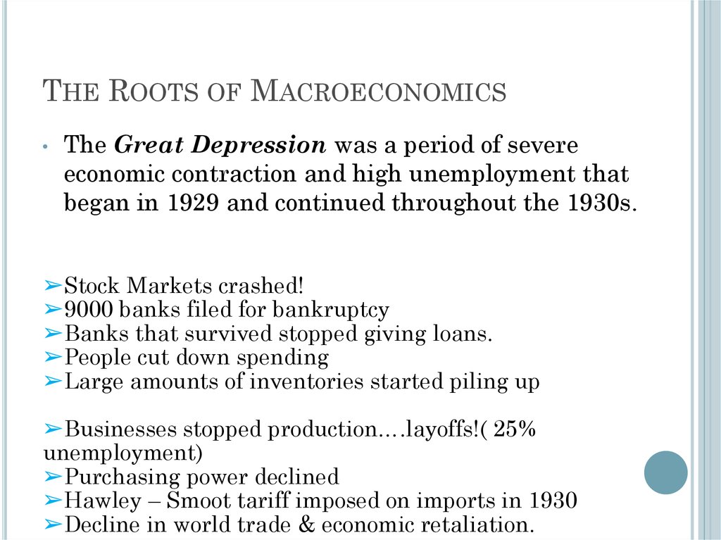
THE ROOTS OF MACROECONOMICSThe Great Depression was a period of severe
economic contraction and high unemployment that
began in 1929 and continued throughout the 1930s.
➢Stock Markets crashed!
➢9000 banks filed for bankruptcy
➢Banks that survived stopped giving loans.
➢People cut down spending
➢Large amounts of inventories started piling up
➢Businesses stopped production….layoffs!( 25%
unemployment)
➢Purchasing power declined
➢Hawley – Smoot tariff imposed on imports in 1930
➢Decline in world trade & economic retaliation.
33.
THE ROOTS OF MACROECONOMICSClassical economists applied
microeconomic models, or “market
clearing” models, to economy-wide
problems.
However, simple classical models
failed to explain the prolonged
existence of high unemployment
during the Great Depression. This
provided the impetus for the
development of macroeconomics
34.
THE ROOTS OF MACROECONOMICSIn 1936, John Maynard
Keynes published The
General Theory of
Employment, Interest, and
Money.
Keynes believed governments
could intervene in the economy
and affect the level of output
and employment.
● During periods of low private
demand, the government can
stimulate aggregate demand to
lift the economy out of
recession.
35.
RECENT MACROECONOMIC HISTORYFine-tuning was the
phrase used by Walter
Heller to refer to the
government’s role in
regulating inflation and
unemployment.
The use of Keynesian
policy to fine-tune the
economy in the 1960s, led
to disillusionment in the
1970s and early 1980s.
36.
WHY TO STUDY MACROECONOMICS?Macroeconomics is the study of the nation’s
economy as a whole.
We can use macroeconomic analysis to:
Understand why economies grow.
● Understand economic fluctuations.
● Make informed business decisions.
37.
MACROECONOMIC CONCERNSThree of the major concerns of macroeconomics
are:
Inflation
● Output growth
● Unemployment
38.
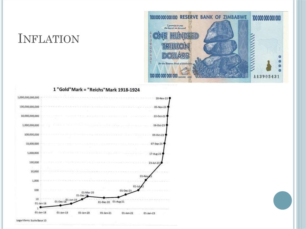
INFLATION AND DEFLATIONInflation is an increase in the overall price
level.
• Hyperinflation is a period of very rapid
increases in the overall price level.
Hyperinflations are rare, but have been used to
study the costs and consequences of even
moderate inflation.
• Deflation is a decrease in the overall price
level. Prolonged periods of deflation can be just
as damaging for the economy as sustained
inflation.
39.
INFLATION40.
OUTPUT GROWTH:SHORT RUN AND LONG RUN
The business cycle is the cycle of short-term
ups and downs in the economy.
The main measure of how an economy is doing is
aggregate output:
Aggregate output is the total quantity of goods
and services produced in an economy in a given
period
41.
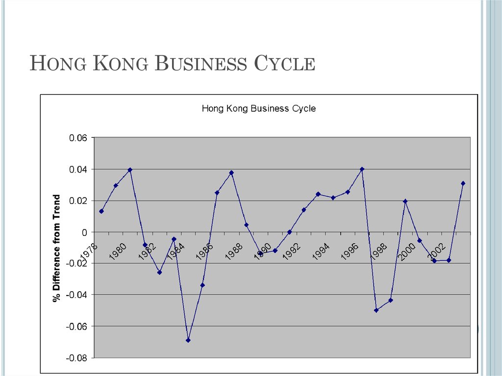
The Business cycle is the riseand fall of economic activity
relative to the long-term
growth trend of the economy
42.
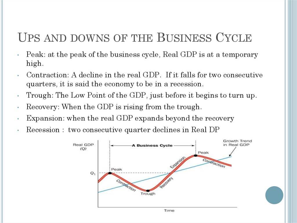
UPS AND DOWNS OF THE BUSINESS CYCLEPeak: at the peak of the business cycle, Real GDP is at a temporary
high.
Contraction: A decline in the real GDP. If it falls for two consecutive
quarters, it is said the economy to be in a recession.
Trough: The Low Point of the GDP, just before it begins to turn up.
Recovery: When the GDP is rising from the trough.
Expansion: when the real GDP expands beyond the recovery
Recession : two consecutive quarter declines in Real DP
43.
RECENT MACROECONOMIC HISTORYStagflation occurs when the overall price
level rises rapidly (inflation) during periods of
recession or high and persistent unemployment
(stagnation).
44.
STAGFLATIONStagflation is a contraction of a nation’s output
accompanied by inflation
Staglation is generally a “supply-side” phenomenon
A dramatic increase in oil prices caused the
stagflation of the 1970s
45.
OUTPUT GROWTH:SHORT RUN AND LONG RUN
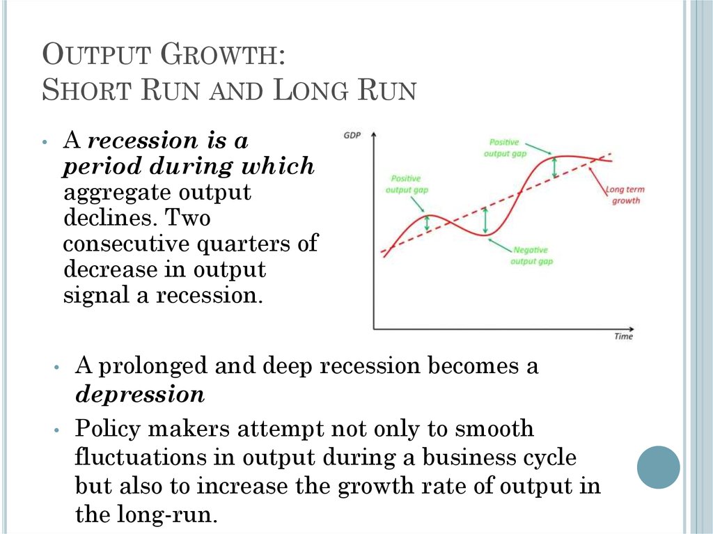
A recession is a
period during which
aggregate output
declines. Two
consecutive quarters of
decrease in output
signal a recession.
A prolonged and deep recession becomes a
depression
Policy makers attempt not only to smooth
fluctuations in output during a business cycle
but also to increase the growth rate of output in
the long-run.
46.
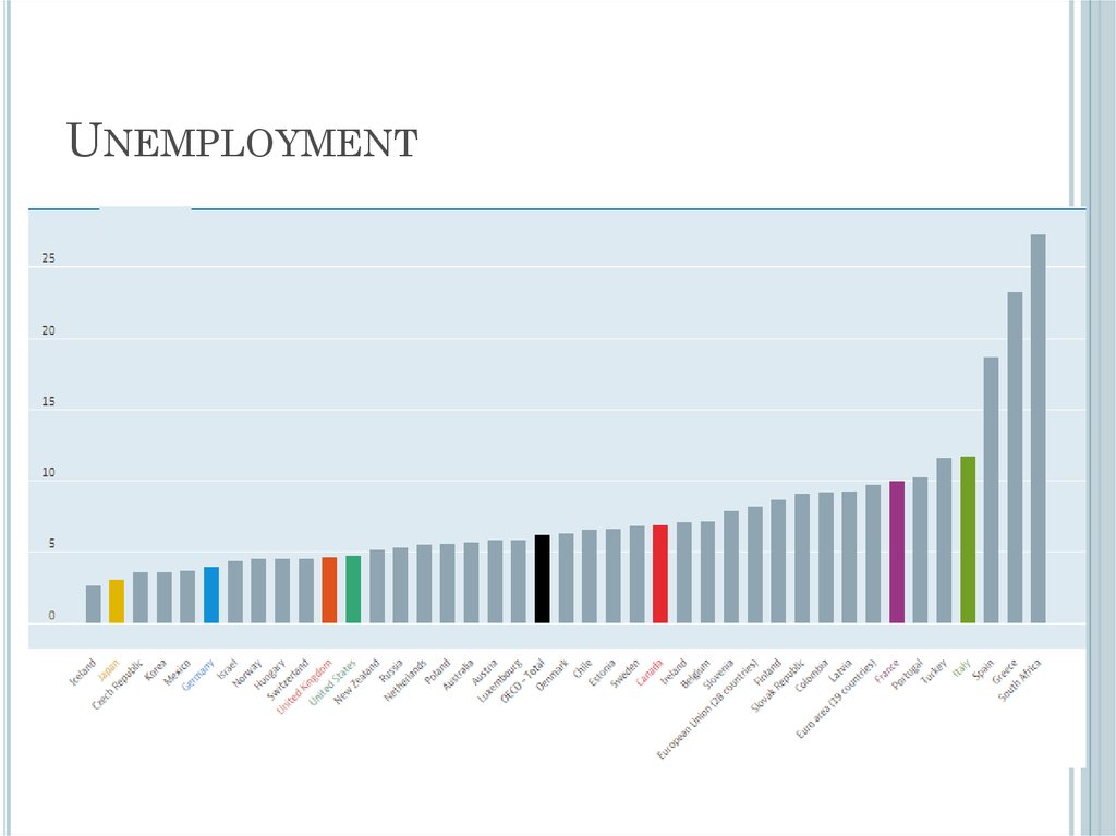
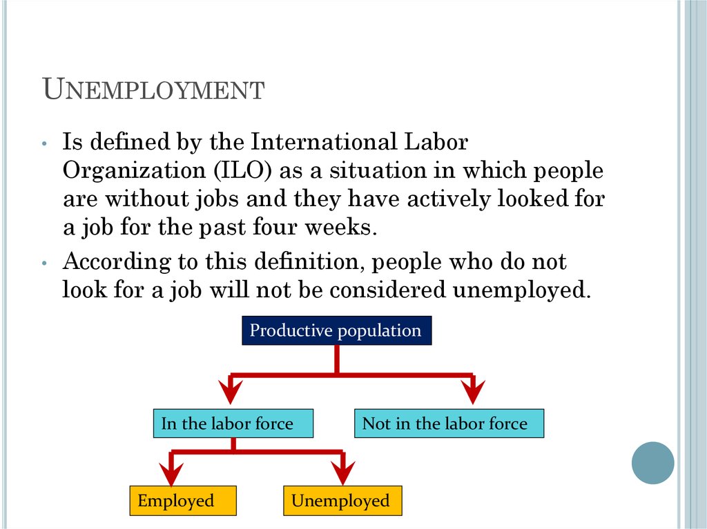
UNEMPLOYMENTThe unemployment rate is the percentage of
the labor force that is unemployed.
The unemployment rate is a key indicator of the
economy’s health.
● The existence of unemployment seems to imply that
the aggregate labor market is not in equilibrium.
● Why do labor markets not clear when other markets
do?
47.
UNEMPLOYMENT48.
GOVERNMENT IN THE MACROECONOMYThere are three kinds of policy that the
government has used to influence the
macroeconomics:
Fiscal policy
● Monetary policy
● Growth or supply-side policies
49.
GOVERNMENT IN THE MACROECONOMYFiscal policy refers to government policies
concerning taxes and spending.
Monetary policy consists of tools used by the
Federal Reserve to control the quantity of money
in the economy.
Growth policies are government policies that
focus on stimulating aggregate supply instead of
aggregate demand.
50.
THE COMPONENTS OF THEMACROECONOMY
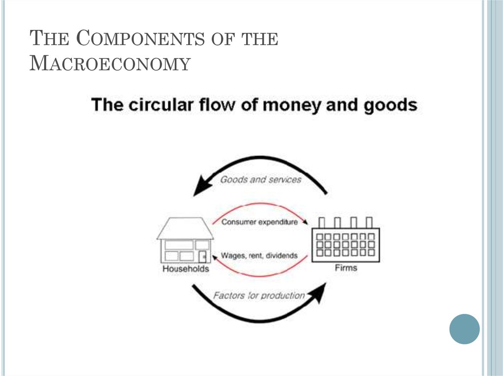
The circular
flow diagram
shows the
income received
and payments
made by each
sector of the
economy.
Everyone’s expenditure is someone else’s
receipt. Every transaction must have two
sides.
51.
THE COMPONENTS OF THEMACROECONOMY
52.
THE COMPONENTS OF THEMACROECONOMY
53.
THE COMPONENTS OF THEMACROECONOMY
Transfer payments are payments made by the
government to people who do not supply goods,
services, or labor in exchange for these payments.
54.
THE THREE MARKET ARENASHouseholds, firms, the government, and the rest
of the world all interact in three different market
arenas:
Goods-and-services market
Labor market
Money (financial) market
55.
THE THREE MARKET ARENASHouseholds and the government purchase goods
and services (demand) from firms in the goodsand services market, and firms supply to the
goods and services market.
In the labor market, firms and government
purchase (demand) labor from households
(supply).
The total supply of labor in the economy depends on
the sum of decisions made by households.
56.
THE THREE MARKET ARENASIn the money market – sometimes called the
financial market – households purchase stocks
and bonds from firms.
Households supply funds to this market in the
expectation of earning income, and also demand
(borrow) funds from this market.
● Firms, government, and the rest of the world also
engage in borrowing and lending, coordinated by
financial institutions.
57.
FINANCIAL INSTRUMENTSTreasury bonds, notes, and bills are
promissory notes issued by the federal
government when it borrows money.
Corporate bonds are promissory notes issued
by corporations when they borrow money
Shares of stock are financial instruments
that give to the holder a share in the firm’s
ownership and therefore the right to share in the
firm’s profits.
Dividends are the portion of a corporation’s profits
that the firm pays out each period to its
shareholders.hen they borrow money.
58.
THE METHODOLOGY OFMACROECONOMICS
Connections to microeconomics:
● Macroeconomic behavior is the sum of all the
microeconomic decisions made by individual
households and firms. We cannot understand
the former without some knowledge of the
factors that influence the latter.
59.
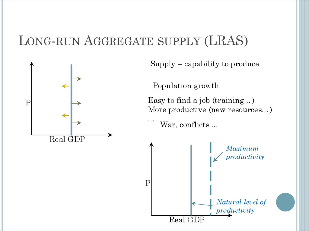
AGGREGATE SUPPLY ANDAGGREGATE DEMAND
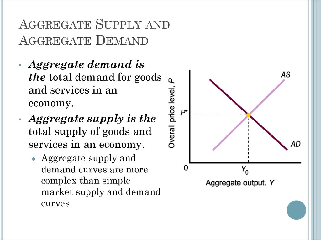
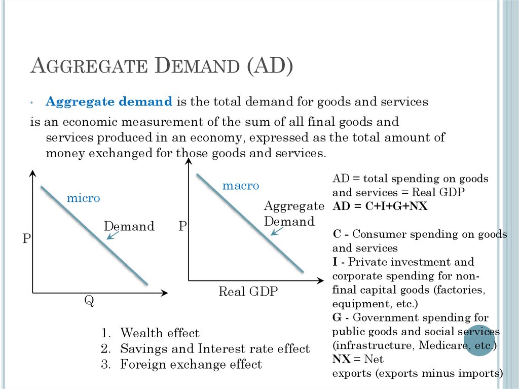
Aggregate demand is
the total demand for goods
and services in an
economy.
Aggregate supply is the
total supply of goods and
services in an economy.
Aggregate supply and
demand curves are more
complex than simple
market supply and demand
curves.
60.
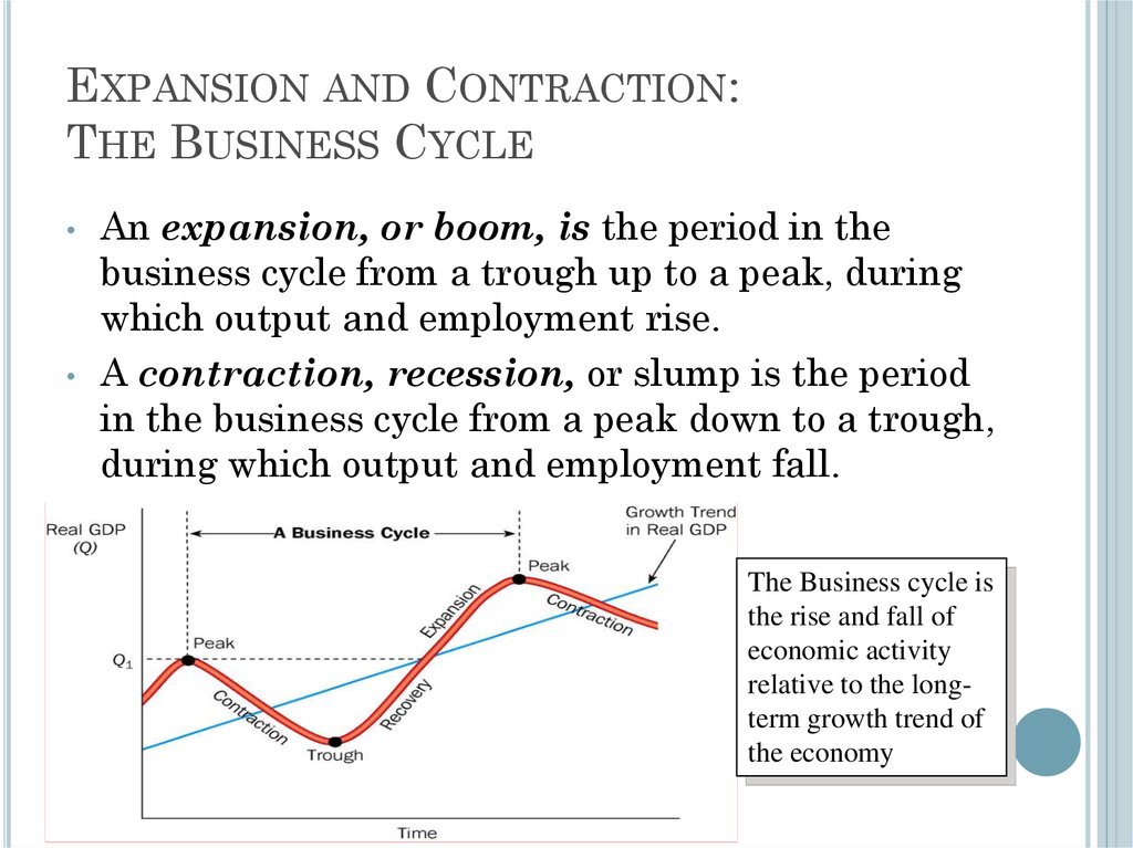
EXPANSION AND CONTRACTION:THE BUSINESS CYCLE
An expansion, or boom, is the period in the
business cycle from a trough up to a peak, during
which output and employment rise.
A contraction, recession, or slump is the period
in the business cycle from a peak down to a trough,
during which output and employment fall.
The Business cycle is
the rise and fall of
economic activity
relative to the longterm growth trend of
the economy
61.
REVIEW TERMS AND CONCEPTSaggregate behavior
aggregate demand
aggregate output
aggregate supply
business cycle
circular flow
contraction, recession, or
slump
corporate bonds
deflation
depression
microeconomics
monetary policy
recession
shares of stock
62.
MACROECONOMICSTHE MEASUREMENT AND
STRUCTURE OF THE
NATIONAL ECONOMY
Zharova Liubov
Zharova_l@ua.fm
63.
OUTLINENational Income Accounting: The Measurement
of Production, Income, and Expenditure
Gross Domestic Product
Saving and Wealth
Real GDP, Price Indexes, and Inflation
Interest Rates
64.
NATIONAL INCOME ACCOUNTINGThe national income accounts is an
accounting framework used in measuring current
economic activity.
The product approach measures the amount of output
produced, excluding output used up in intermediate
stages of production.
The income approach measures the incomes received
by the producers of output
65.
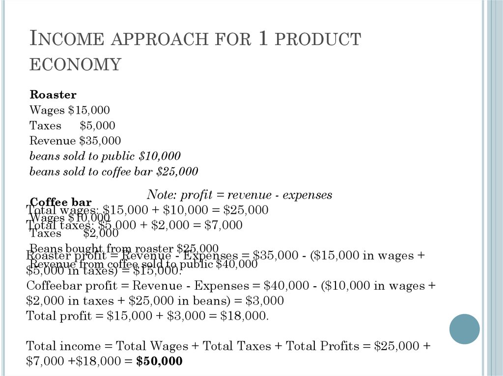
NATIONAL INCOME ACCOUNTINGBusiness example shows that all three
approaches are equal
Important concept in product approach:
(Value
added)
= (Value of
output)
–
(Value of inputs
purchased from
other producers)
66.
NATIONAL INCOME ACCOUNTINGWhy are the three approaches equivalent?
● They must be, by definition
● Any output produced (product approach) is
purchased by someone (expenditure approach)
and results in income to someone (income
approach)
The fundamental identity of national income
accounting:
total production = total income = total
expenditure
67.
NATIONAL INCOME ACCOUNTINGSome of the metrics calculated by using national
income accounting include
Gross Domestic Product (GDP)
Gross National Product (GNP)
Gross National Income (GNI).
68.
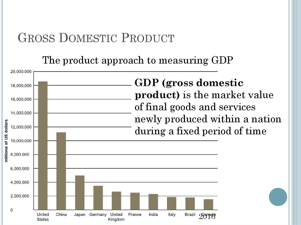
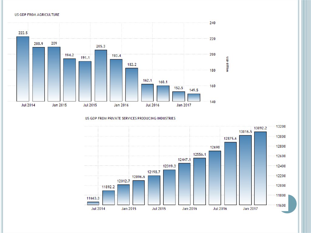
GROSS DOMESTIC PRODUCTThe product approach to measuring GDP
GDP (gross domestic
product) is the market value
of final goods and services
newly produced within a nation
during a fixed period of time
2016
69.
GROSS DOMESTIC PRODUCTMarket value: allows adding together unlike
items by valuing them at their market prices
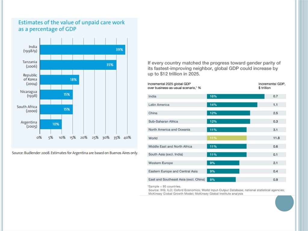
● Problem: misses nonmarket items such as
homemaking, the value of environmental
quality, and natural resource depletion
● There is some adjustment to reflect the
underground economy
● Government services (that aren’t sold in
markets) are valued at their cost of production
70.
71.
GDPNewly produced: counts only things produced in the
given period; excludes things produced earlier
Final goods and services* - are those that are not
intermediate
*Don’t count intermediate goods and services (those used up in the
production of other goods and services in the same period that
they themselves were produced)
Capital goods (goods used to produce other goods)
are final goods since they aren’t used up in the
same period that they are produced
● Inventory investment (the amount that
inventories of unsold finished goods, goods in
process, and raw materials have changed during
the period) is also treated as a final good
● Adding up value added works well, since it
automatically excludes intermediate goods
72.
GNPGNP (Gross National Product) = output produced
by domestically owned factors of production
GDP = output produced within a nation
GDP = GNP – NFP
NFP – Net Factor Payments from abroad
NFP
= (Payments to
domestically owned
factors located
abroad)
- (Payments to
foreign factors
located
domestically)
73.
GNPExample: Engineering revenues for a road built
by a U.S. company in Saudi Arabia is part of U.S.
GNP (built by a U.S. factor of production), not
U.S. GDP, and is part of Saudi GDP (built in
Saudi Arabia), not Saudi GNP
Difference between GNP and GDP is small for
the United States, about 0.2%, but higher for
countries that have many citizens working
abroad
74.
EXAMPLEIf a Japanese multinational produces cars in the UK, this
production will be counted towards UK GDP. However, if the
Japanese firm sends £50m in profits back to shareholders in
Japan, then this outflow of profit is subtracted from GNP. UK
nationals don’t benefit from this profit which is sent back to
Japan.
If a UK firm makes a profit from insurance companies located
abroad, then if this profit is returned to UK nationals, then this
net income from overseas assets will be added to UK GNP.
Note, if a Japanese firm invests in the UK, it will still lead to
higher GNP, as some national workers will see higher wages.
However, the increase in GNP will not be as high as GDP.
If a county has similar inflows and outflows of income from
assets, then GNP and GDP will be very similar.
However, if a country has many multinationals who repatriate
income from local production, then GNP will be lower than
GDP. For example, Luxembourg has a GDP of $87,400 but a
GNP of only $45,360.
75.
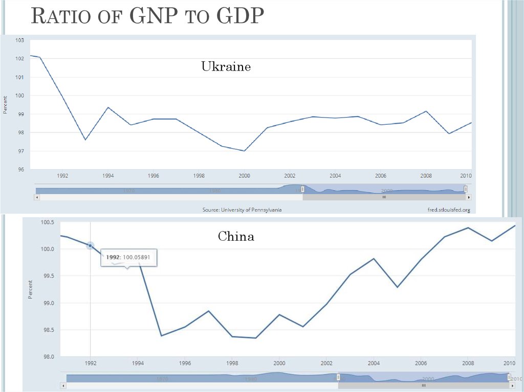
RATIO OF GNP TO GDPUkraine
China
76.
GNIGNI (Gross National Income) – measures income received
by a country both domestically and from overseas.
GNI = GDP + Net Income received from overseas
GNI
= Value
+
added by all
producers who
are residents
in a nation
Product taxes
(minus
subsidies) not
included in
output
+
Income received from
abroad (employee
compensation and
property income)
77.
GNIFor most nations there is little difference
between GDP and GNI
GNI for the U.S. about 1.5% higher than GDP.
GNI can be well below GDP
Ireland, since large-scale repatriation of profits from
foreign companies located there far exceeds income
flows from overseas. Ireland’s GNI was 20% below its
GDP, which means that although Ireland attracts
substantial foreign investment that contributes to
its economic growth, a big chunk of the profits arising
from such foreign investment does not remain in the
nation. In this case, GNI may be a better indicator of
Ireland’s economic performance than GDP, since the
latter overstates the strength of the Irish economy.
78.
TO CONVERT A NATION’S GDP TO GNIThree terms need to be added to the former:
net compensation receipts,
● net property income receivable
● net taxes (minus subsidies) receivable on production
and imports.
GDP(Canada) = $1,624.6 million
Net compensation receipts = 0
Net property income receivable = - $28.2 million
Net taxes = 0
GNI(Canada) = $1,624.6 + (-28.2) = $1,596.4
million
79.
Income Earnedby:
Residents in
Country
GDP
GNI
GNP
Personal
GDP + (income
GDP +(income from
consumption (C) + citizens and businesses earned on all foreign
business investment
assets) – (income
earned abroad) –
(I) + government
earned by foreigners
(income remitted by
spending (G) +
in the country)
foreigners living in the
[exports - imports
country back to their
(X)]
home countries)
___________________
GNP + (income spent by
foreigners within the
country) – (foreign
income not remitted by
citizens)
Foreigners in
Country
Includes
Includes If Spent in
Country
Excludes All
Residents Out
of Country
Excludes
Includes If Remitted
Back
Includes All
Foreigners Out
of Country
Excludes
Excludes
Excludes
80.
81.
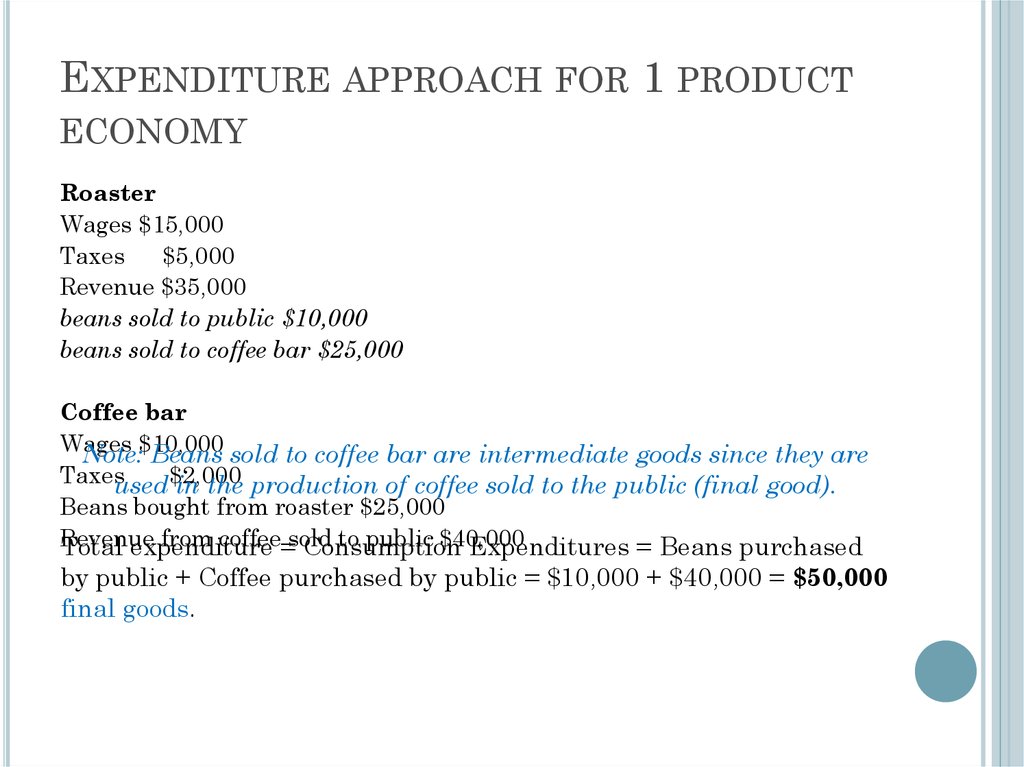
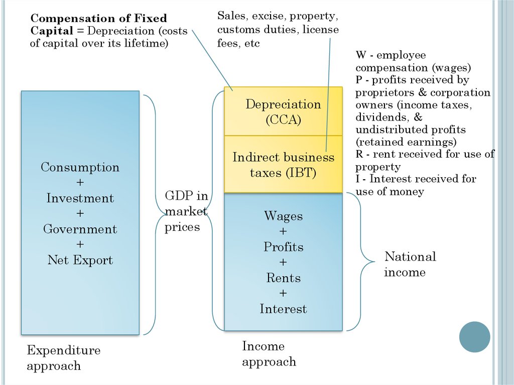
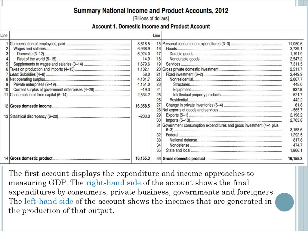
GDP MEASUREMENTThe expenditure approach to measuring GDP
Measures total spending on final goods and
services produced within a nation during a
specified period of time
Four main categories of spending: consumption
(C), investment (I), Government purchases of
goods and services (G), and net exports (NX)
Y = C + I + G + NX
the income-expenditure identity
● exports minus imports
82.
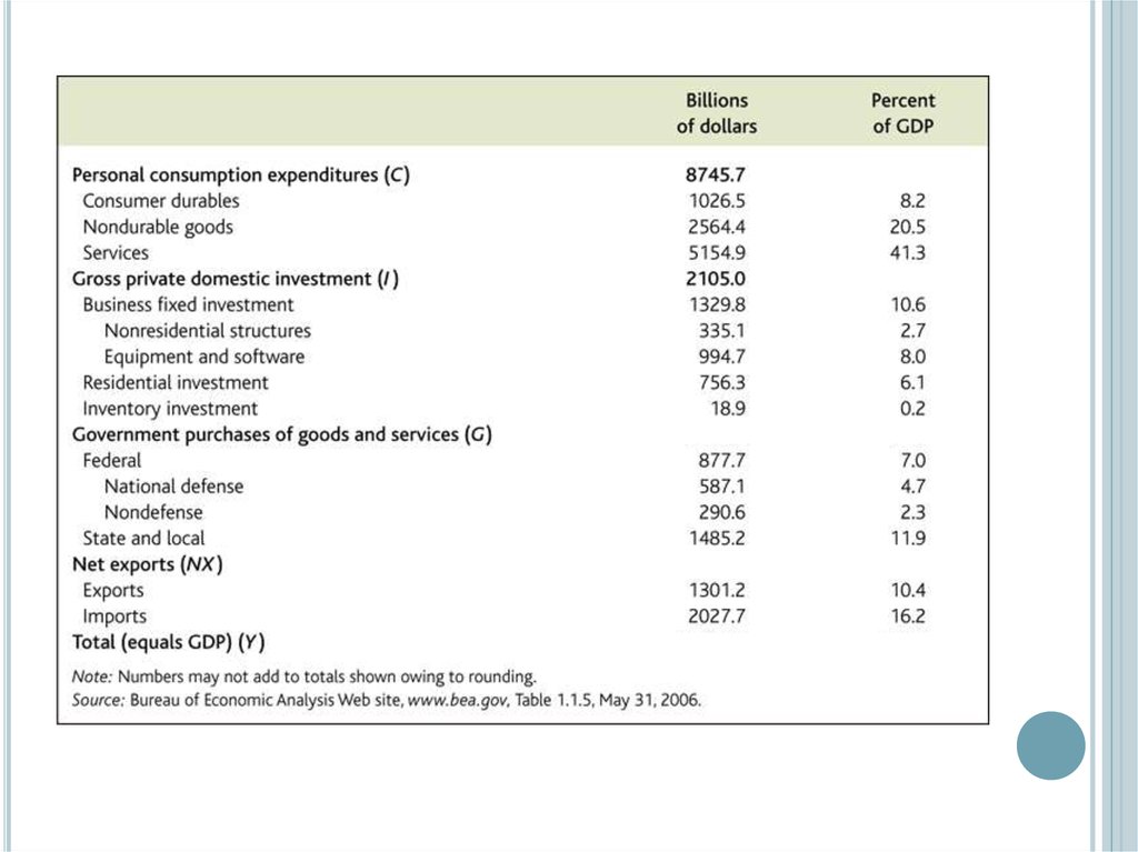
GDP MEASUREMENT /EXPENDITURE APPROACH
Consumption: spending by domestic households
on final goods and services (including those
produced abroad)
● About 2/3 of U.S. GDP
● Three categories:
• Consumer durables (examples: cars, TV sets,
furniture, major appliances)
• Nondurable goods (examples: food, clothing,
fuel)
• Services (examples: education, health care,
financial services, transportation)
83.
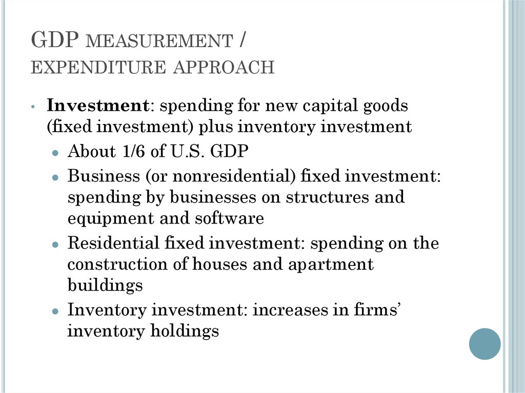
GDP MEASUREMENT /EXPENDITURE APPROACH
Investment: spending for new capital goods
(fixed investment) plus inventory investment
● About 1/6 of U.S. GDP
● Business (or nonresidential) fixed investment:
spending by businesses on structures and
equipment and software
● Residential fixed investment: spending on the
construction of houses and apartment
buildings
● Inventory investment: increases in firms’
inventory holdings
84.
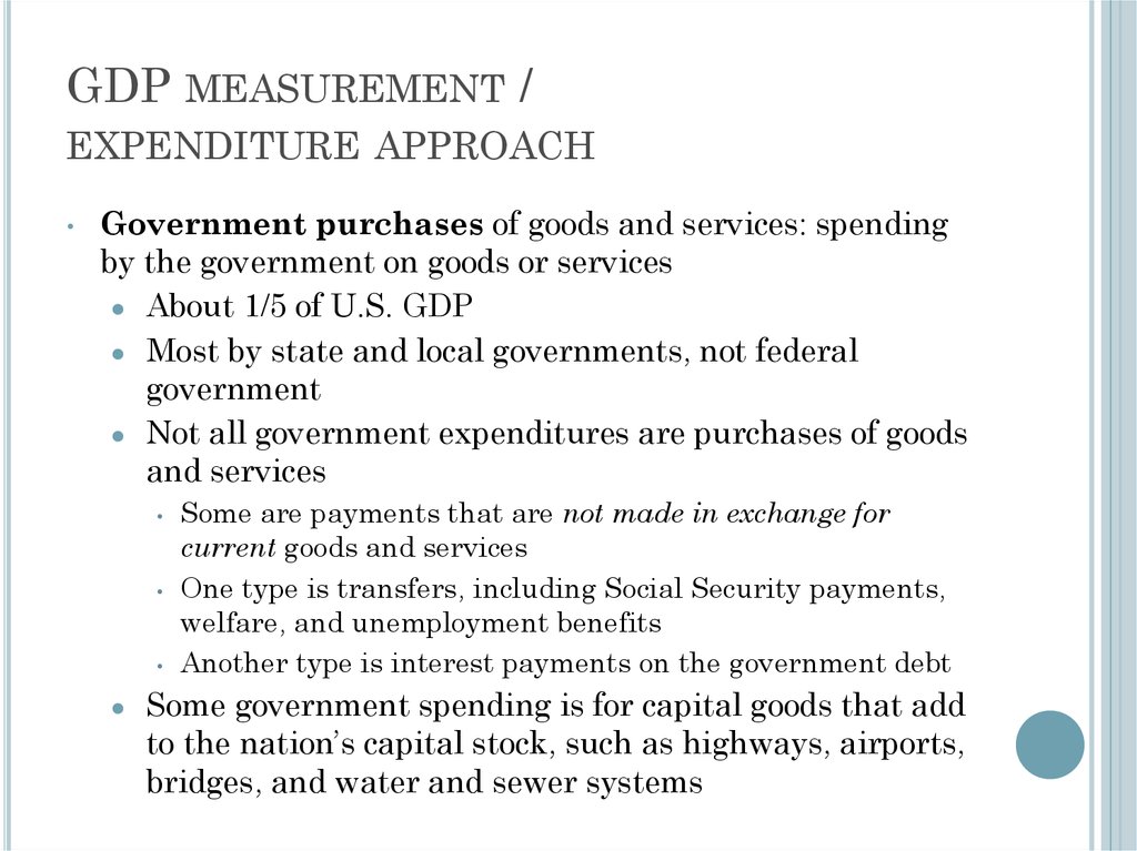
GDP MEASUREMENT /EXPENDITURE APPROACH
Government purchases of goods and services: spending
by the government on goods or services
● About 1/5 of U.S. GDP
● Most by state and local governments, not federal
government
● Not all government expenditures are purchases of goods
and services
Some are payments that are not made in exchange for
current goods and services
One type is transfers, including Social Security payments,
welfare, and unemployment benefits
Another type is interest payments on the government debt
Some government spending is for capital goods that add
to the nation’s capital stock, such as highways, airports,
bridges, and water and sewer systems
85.
GDP MEASUREMENT /EXPENDITURE APPROACH
Net exports: exports minus imports
● Exports: goods produced in the country that
are purchased by foreigners
● Imports: goods produced abroad that are
purchased by residents in the country
● Imports are subtracted from GDP, as they
represent goods produced abroad, and were
included in consumption, investment, and
government purchases
86.
EXPENDITURE APPROACH TO MEASURINGGDP (UNITED STATES)
87.
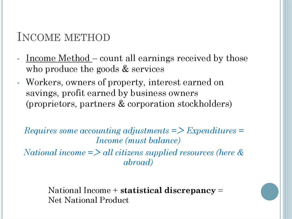
GDP MEASUREMENT /INCOME APPROACH
Adds up income generated by production
(including profits and taxes paid to the
government)
National Income = (compensation of employees
(including benefits) + (proprietors’ income) + (rental
income of persons) + (corporate profits) + (net
interest) + (taxes on production and imports) +
(business current transfer payments) + (current
surplus of government enterprises)
● National income + statistical discrepancy = Net
National Product
● Net National Product + Depreciation (the value of
capital that wears out in the period) = Gross National
Product (GNP)
● GNP – Net Factor Payments (NFP) = GDP
88.
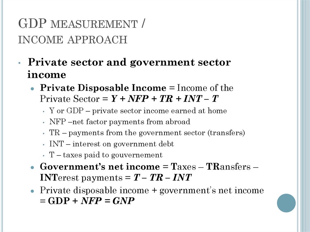
GDP MEASUREMENT /INCOME APPROACH
Private sector and government sector
income
Private Disposable Income = Income of the
Private Sector = Y + NFP + TR + INT – T
Y or GDP – private sector income earned at home
NFP –net factor payments from abroad
TR – payments from the government sector (transfers)
INT – interest on government debt
T – taxes paid to gouvernement
Government’s net income = Taxes – TRansfers –
INTerest payments = T – TR – INT
● Private disposable income + government’s net income
= GDP + NFP = GNP
89.
INCOME APPROACH TO MEASURING GDP(US)
90.
SAVING AND WEALTHWealth
● Household Wealth = (Household’s Assets) –
(Household’s Liabilities)
● National Wealth = sum of all households’,
firms’, and governments’ wealth within the
nation
● Saving by individuals, businesses, and
government determine wealth
91.
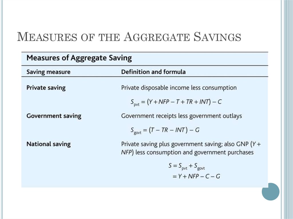
SAVING AND WEALTH /MEASURES OF AGGREGATE SAVING
Saving = Current Income – Current Spending
Saving Rate = Saving / Current Income
Private Saving = Private disposable income –
Consumption
Spvt = (Y + NFP – T + TR + INT) – C
92.
SAVING AND WEALTH /MEASURES OF AGGREGATE SAVING
Government Saving = Net Government Income
– Government purchases of goods and services
Sgovt = (T – TR – INT) – G
Government saving = government budget surplus
= Government Receipts – Government Outlays
Government receipts = Tax revenue (T)
● Government outlays = Government purchases of goods
and services (G) + TRansfers (TR) + INTerest
payments on government debt (INT)
Government budget deficit = – Sgovt
Simplification: count government investment as government
purchases, not investment
93.
SAVING AND WEALTH /MEASURES OF AGGREGATE SAVING
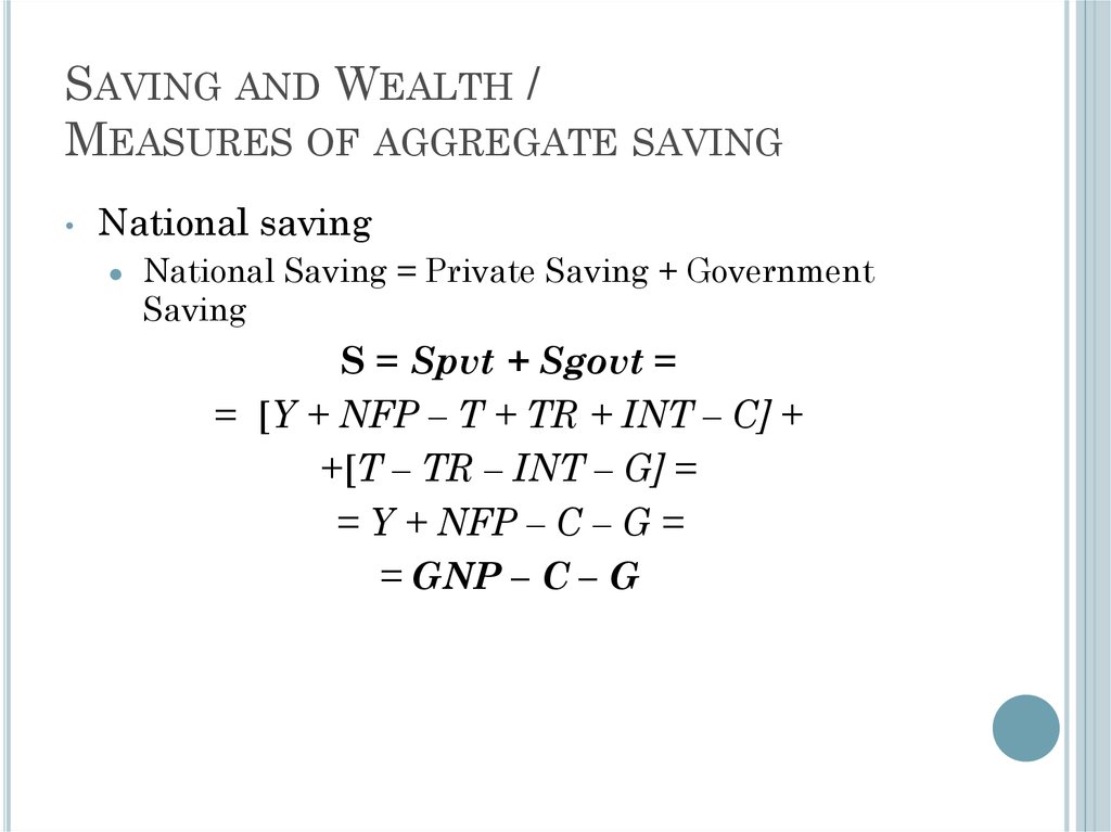
National saving
National Saving = Private Saving + Government
Saving
S = Spvt + Sgovt =
= [Y + NFP – T + TR + INT – C] +
+[T – TR – INT – G] =
= Y + NFP – C – G =
= GNP – C – G
94.
SAVING AND WEALTH /MEASURES OF AGGREGATE SAVING
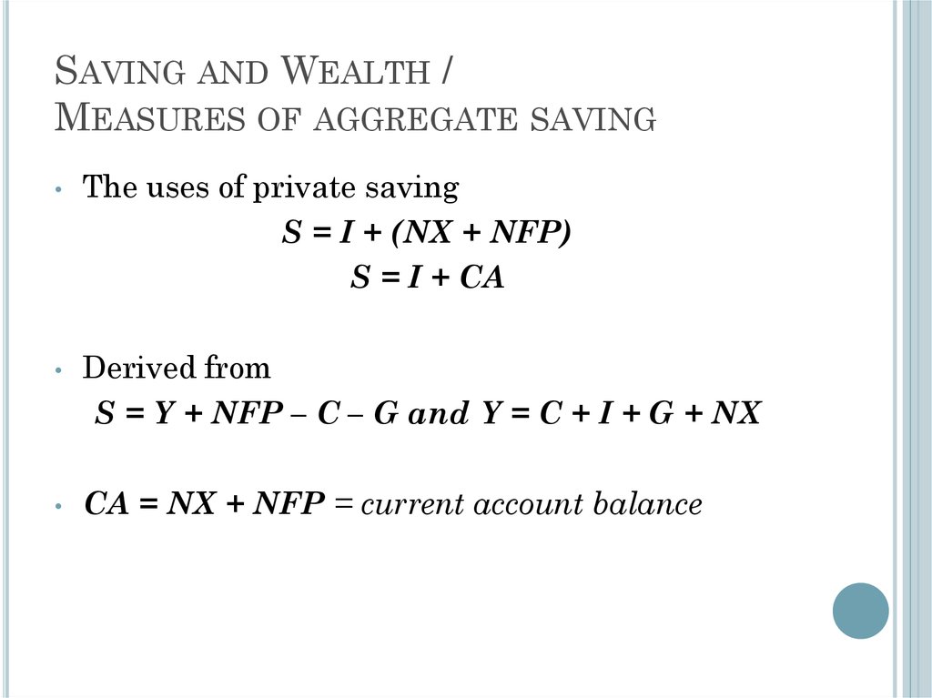
The uses of private saving
S = I + (NX + NFP)
S = I + CA
Derived from
S = Y + NFP – C – G and Y = C + I + G + NX
CA = NX + NFP = current account balance
95.
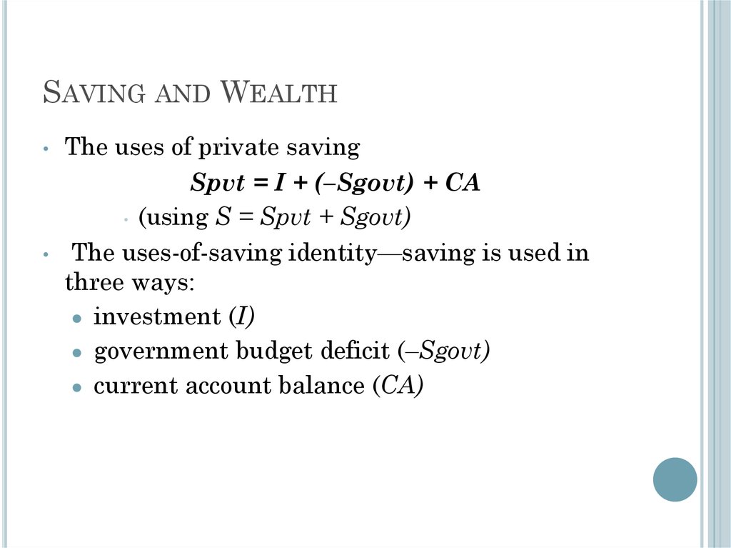
SAVING AND WEALTHThe uses of private saving
Spvt = I + (–Sgovt) + CA
• (using S = Spvt + Sgovt)
The uses-of-saving identity—saving is used in
three ways:
● investment (I)
● government budget deficit (–Sgovt)
● current account balance (CA)
96.
SAVING AND WEALTH /RELATING SAVING AND WEALTH
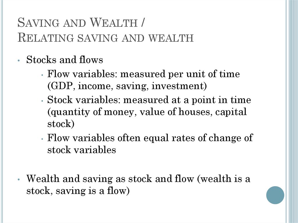
Stocks and flows
• Flow variables: measured per unit of time
(GDP, income, saving, investment)
• Stock variables: measured at a point in time
(quantity of money, value of houses, capital
stock)
• Flow variables often equal rates of change of
stock variables
Wealth and saving as stock and flow (wealth is a
stock, saving is a flow)
97.
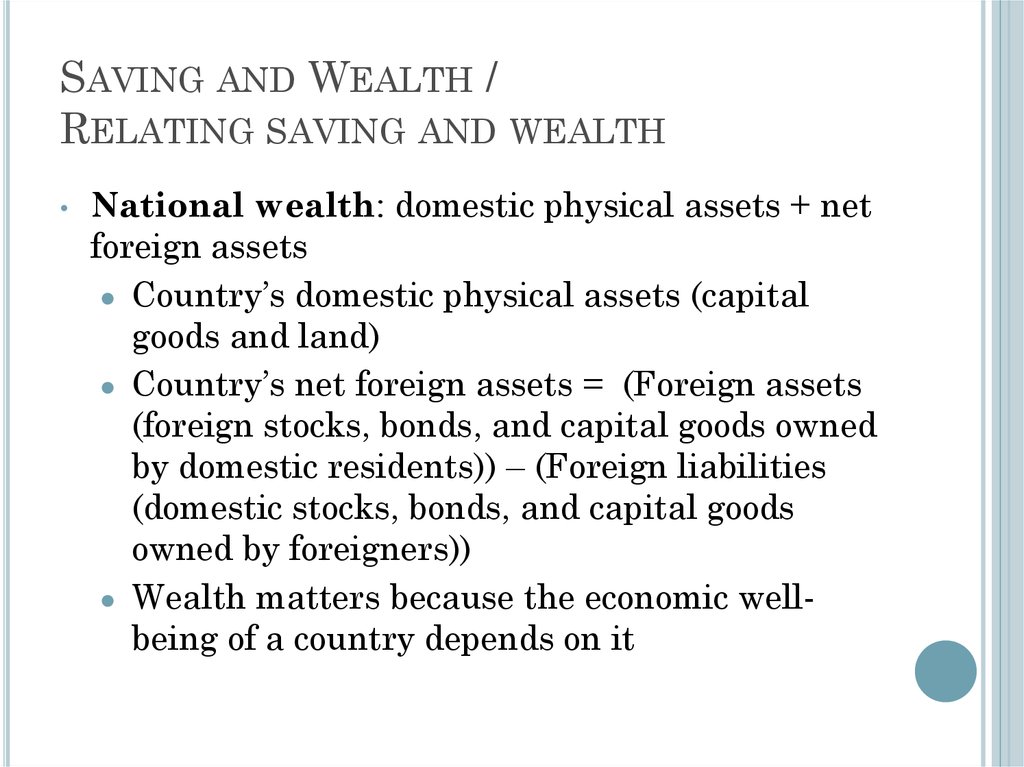
SAVING AND WEALTH /RELATING SAVING AND WEALTH
National wealth: domestic physical assets + net
foreign assets
● Country’s domestic physical assets (capital
goods and land)
● Country’s net foreign assets = (Foreign assets
(foreign stocks, bonds, and capital goods owned
by domestic residents)) – (Foreign liabilities
(domestic stocks, bonds, and capital goods
owned by foreigners))
● Wealth matters because the economic wellbeing of a country depends on it
98.
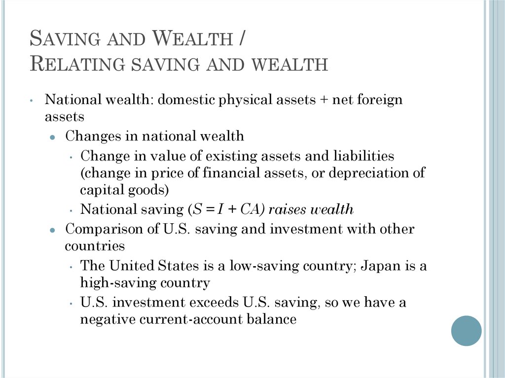
SAVING AND WEALTH /RELATING SAVING AND WEALTH
National wealth: domestic physical assets + net foreign
assets
● Changes in national wealth
• Change in value of existing assets and liabilities
(change in price of financial assets, or depreciation of
capital goods)
• National saving (S = I + CA) raises wealth
● Comparison of U.S. saving and investment with other
countries
• The United States is a low-saving country; Japan is a
high-saving country
• U.S. investment exceeds U.S. saving, so we have a
negative current-account balance
99.
MEASURES OF THE AGGREGATE SAVINGS100.
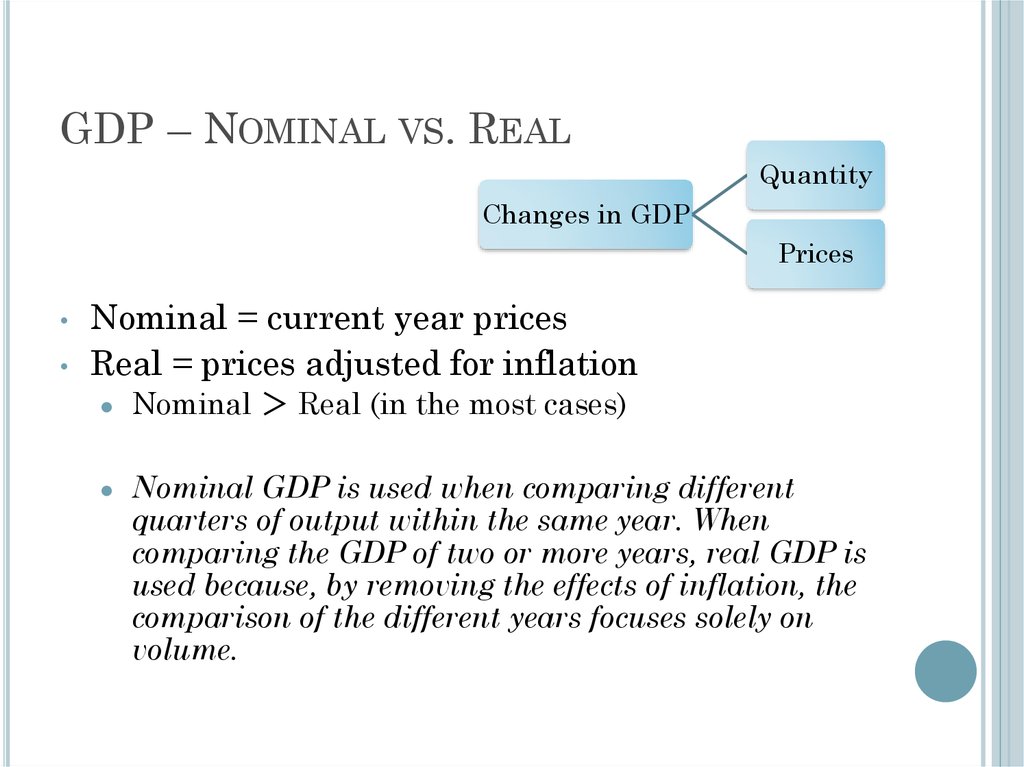
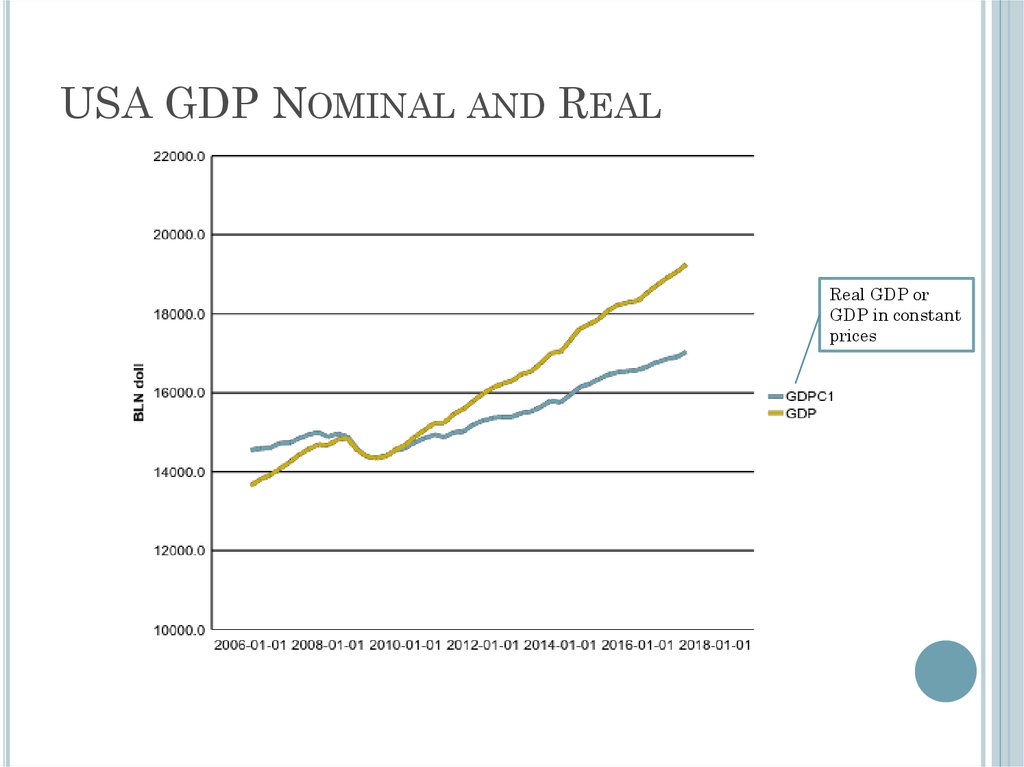
REAL GDP, PRICE INDEXES, ANDINFLATION
Real GDP
● Nominal variables are those in dollar terms
● Problem: Do changes in nominal values reflect
changes in prices or quantities?
● Real variables: adjust for price changes; reflect
only quantity changes
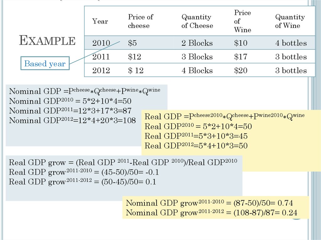
Nominal GDP is the dollar value of an economy’s
final output measured at current market prices
Real GDP is an estimate of the value of an
economy’s final output, adjusting for changes in
the overall price level
101.
COMPUTERS & BICYCLES102.
COMPUTERS & BICYCLES103.
REAL GDP, PRICE INDEXES, ANDINFLATION
Price Indexes
● A price index measures the average level of
prices for some specified set of goods and
services, relative to the prices in a specified
base year
● GDP deflator = 100 × nominal GDP/real GDP
● Note that base year P = 100
104.
REAL GDP, PRICE INDEXES, ANDINFLATION
Price Indexes
● Consumer Price Index (CPI)
Price index is a normalized average (typically a
weighted average) of price relatives for a given
class of goods or services in a given region, during
a given interval of time. It is a statistic designed
to help to compare how these price relatives,
taken as a whole, differ between time periods or
geographical locations.
105.
REAL GDP, PRICE INDEXES, ANDINFLATION
Price Indexes
● GDP
• Choice of expenditure base period matters
for GDP when prices and quantities of a
good, such as computers, are changing
rapidly
• BEA (Bureau of Economic Analysis)
compromised by developing chain-weighted
GDP
• Now, however, components of real GDP don’t
add up to real GDP, but discrepancy is
usually small
106.
REAL GDP, PRICE INDEXES, ANDINFLATION
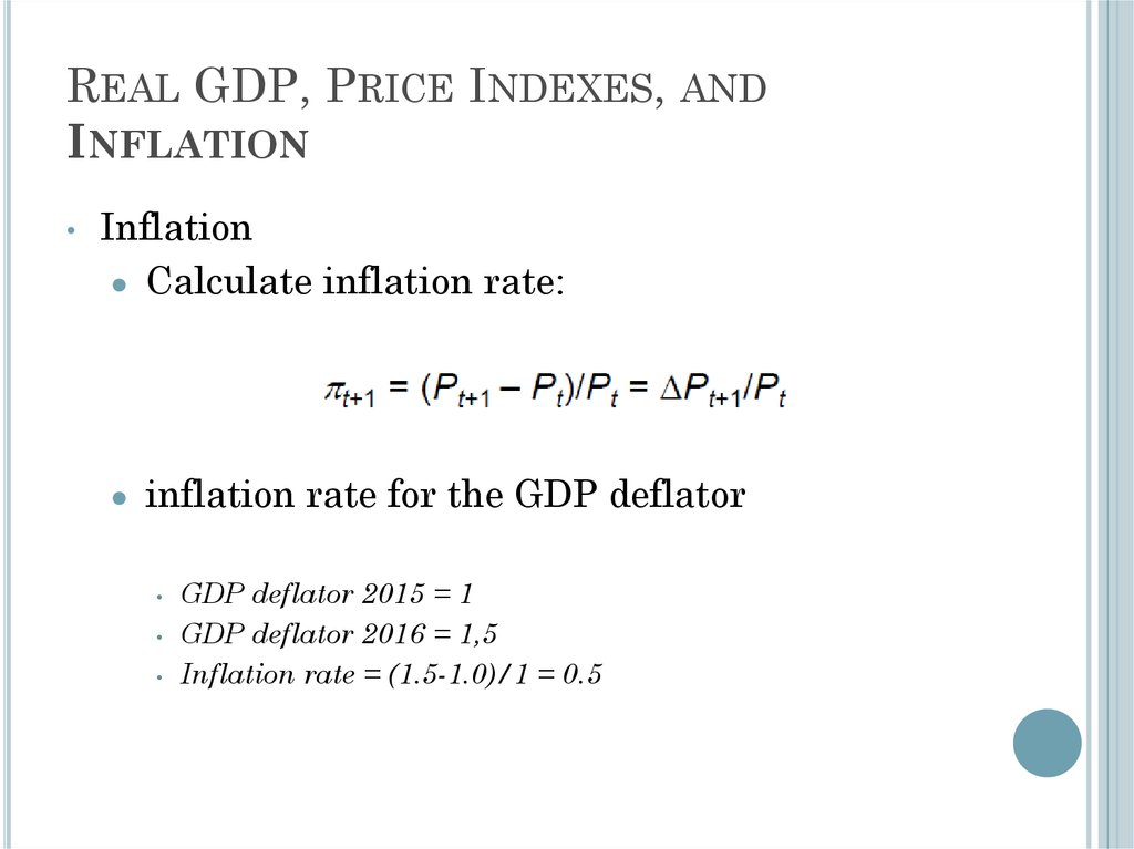
Inflation
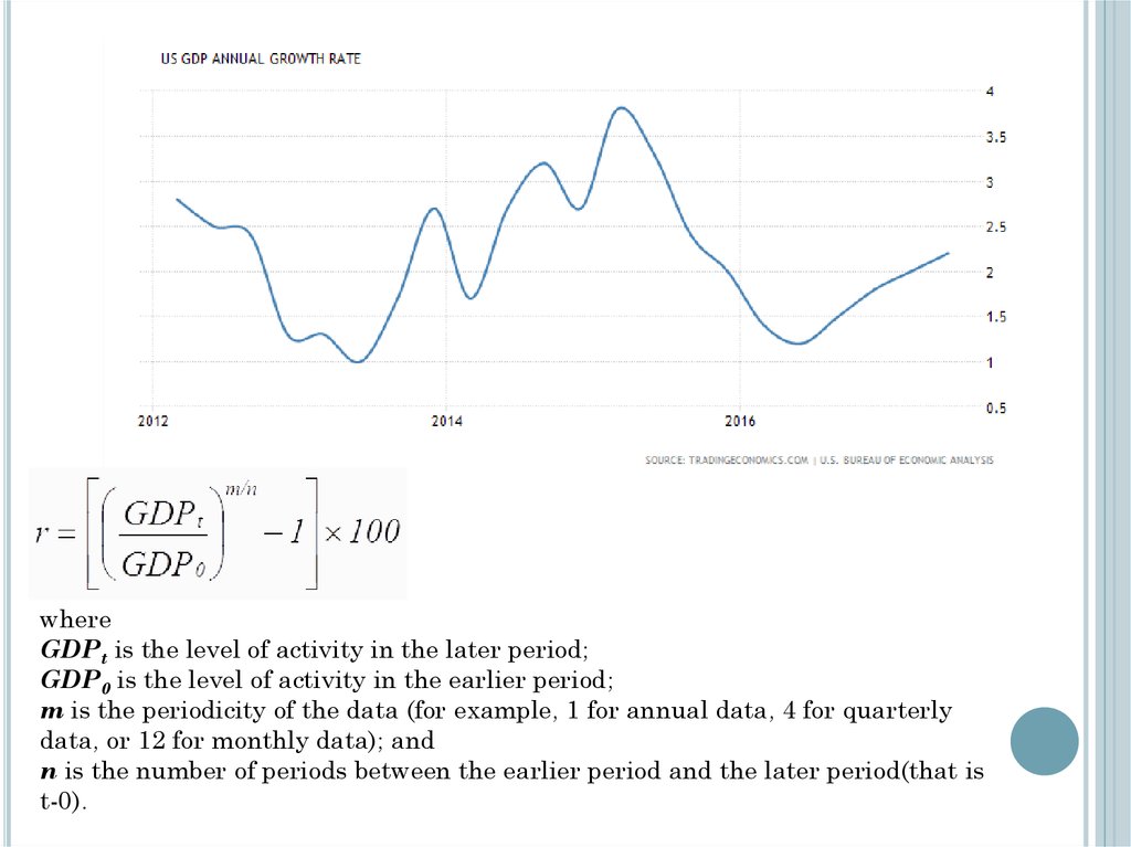
● Calculate inflation rate:
inflation rate for the GDP deflator
GDP deflator 2015 = 1
GDP deflator 2016 = 1,5
Inflation rate = (1.5-1.0)/1 = 0.5
107.
REAL GDP, PRICE INDEXES, ANDINFLATION
Price Indexes
● Does CPI inflation overstate increases in the
cost of living?
The Boskin Commission reported that the CPI was
biased upwards by as much as one to two percentage
points per year
One problem is that adjusting the price measures for
changes in the quality of goods is very difficult
A consumer price index (CPI) measures changes in the
price level of a market basket of consumer goods and
services purchased by households
108.
REAL GDP, PRICE INDEXES, ANDINFLATION
Price Indexes
● Does CPI inflation overstate increases in the
cost of living?
• Price indexes with fixed sets of goods don’t
reflect substitution by consumers when one
good becomes relatively cheaper than
another
● This problem is known as substitution bias
109.
REAL GDP, PRICE INDEXES, ANDINFLATION
Does CPI inflation overstate increases in the cost
of living?
If inflation is overstated, then real incomes are
higher than we thought and we’ve over indexed
payments like Social Security
● Latest research suggests bias is still 1% per year or
higher
110.
INTEREST RATEReal vs. nominal interest rates
● Interest rate: a rate of return promised by a
borrower to a lender
● Real interest rate: rate at which the real value
of an asset increases over time
● Nominal interest rate: rate at which the
nominal value of an asset increases over time
The expected real interest rate
If
,
real interest rate = expected real interest rate
111.
GROSS NATIONAL PRODUCT (GNP)GROSS DOMESTIC PRODUCT (GDP)
NET NATIONAL PRODUCT (NNP)
NET NATIONAL INCOME (NNI)
Gross National Product (GNP) is the total value of
final goods and services produced in a year by
domestically owned factors of production
• Gross Domestic Product (GDP) is the total value of
final goods and services produced within a country's
borders in a year
• NNP equals the GDP minus depreciation on a
country's capital goods
• NNP – Indirect Taxes = Net National Income (NNI),
it encompasses the income of households, businesses,
and the government. It can be expressed as:
NNI = C + I + G + (NX) + net foreign factor income
- indirect taxes - depreciation
112.
THE BALANCE OF PAYMENTS, ALSO KNOWNAS BALANCE OF INTERNATIONAL PAYMENTS
OF A COUNTRY IS THE RECORD OF ALL
ECONOMIC TRANSACTIONS BETWEEN THE
RESIDENTS OF THE COUNTRY AND THE REST OF
THE WORLD IN A PARTICULAR PERIOD
The current account shows the net amount a
country is earning if it is in surplus, or spending
if it is in deficit
The capital account records the net change in
ownership of foreign assets
The IMF definition of Balance of Payment
113.
PRODUCER PRICE INDEX (PPI) MEASURESTHE AVERAGE CHANGES IN PRICES RECEIVED
BY DOMESTIC PRODUCERS FOR THEIR OUTPUT
It is one of several price indexes
● Consumer price index
● Producer price index
● Export price index
● Import price index
● GDP deflator
114.
MACROECONOMICSTHE MEASUREMENT AND
STRUCTURE OF THE
NATIONAL ECONOMY
Zharova Liubov
Zharova_l@ua.fm
115.
116.
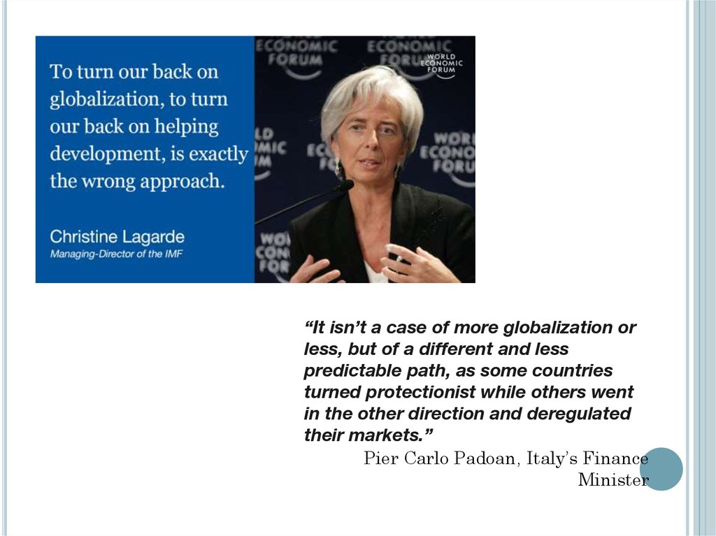
“It isn’t a case of more globalization orless, but of a different and less
predictable path, as some countries
turned protectionist while others went
in the other direction and deregulated
their markets.”
Pier Carlo Padoan, Italy’s Finance
Minister
117.
WHAT IS GLOBALIZATIONGlobalization is defined as a process that, based
on international strategies, aims to expand
business operations on a worldwide level, and
was precipitated by the facilitation of global
communications due to technological
advancements, and socioeconomic, political and
environmental developments.
economic globalization
● cultural globalization
● political globalization
118.
BASIC ASPECTS OF GLOBALIZATIONIn 2000, the International Monetary Fund
(IMF) identified four basic aspects of globalization:
• trade and transactions,
• capital and investment movements,
• migration and movement of people,
• the dissemination of knowledge.
Environmental challenges (global warming,
cross-boundary water and air pollution, and
overfishing of the ocean)
119.
GLOBALIZATION ENCOMPASSESInternationalization (trade & investment)
Liberalization (freeing markets)
Universalization (cultural interchange)…or…
Westernization (Western cultural dominance)
“Deterritorialization” (the severance of social,
political, or cultural practices from their native
places and populations)
120.
IMPACTEconomic impact
Improvement in standard of living
● Increased competition among nations
● Widening income gap between the rich and poor
Social impact
Increased awareness of foreign cultures
● Loss of local culture
Environmental impact
Environmental degradation
● Environmental management
121.
FOCUS ON: MEASURING GLOBALISATIONSTATISTICAL INDICATORS
OECD Economic Globalization Indicators helps
identify the economic activities of member countries
that are under foreign control, and more particularly
the contribution of multinational enterprises to
growth, employment, productivity, labour
compensation, research and development, technology
diffusion and international trade. These indicators
shed new light on financial, technological and trade
interdepe
● World Development Indicators (WDI). The WDI
affords readers more than 900 indicators organized in
six sections: World View, People, Environment,
Economy, States and Markets, and Global Links. In
each section a plethora of information is presented.
ndencies within OECD countries.
122.
FOCUS ON: MEASURING GLOBALISATIONSTATISTICAL INDICATORS
UNCTAD Development and Globalization: Facts and
Figures. This publication covers subjects tackled by
UNCTAD such as trade, investment, external
finance, commodities and manufactures, together
with relevant facts about population.
● Global Policy Forum (GPF) gathers a large
number of tables and graphs providing the main
features of globalization, asking what is new, what
drives the process, how it changes politics, and how it
affects global institutions like UN. In addition to
indicators of social and economic policy, trade and
capital flows, global poverty and development etc.
123.
FOCUS ON: MEASURING GLOBALISATIONCOMPOSITE INDEXES
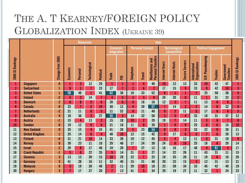
The A. T Kearney/FOREIGN POLICY Globalization
Index (2016 – the last data, in free access up to 2006)
● Centre for the Study of Globalisation and
Regionalisation (CSGR) Globalisation Index (2004 –
the last data)
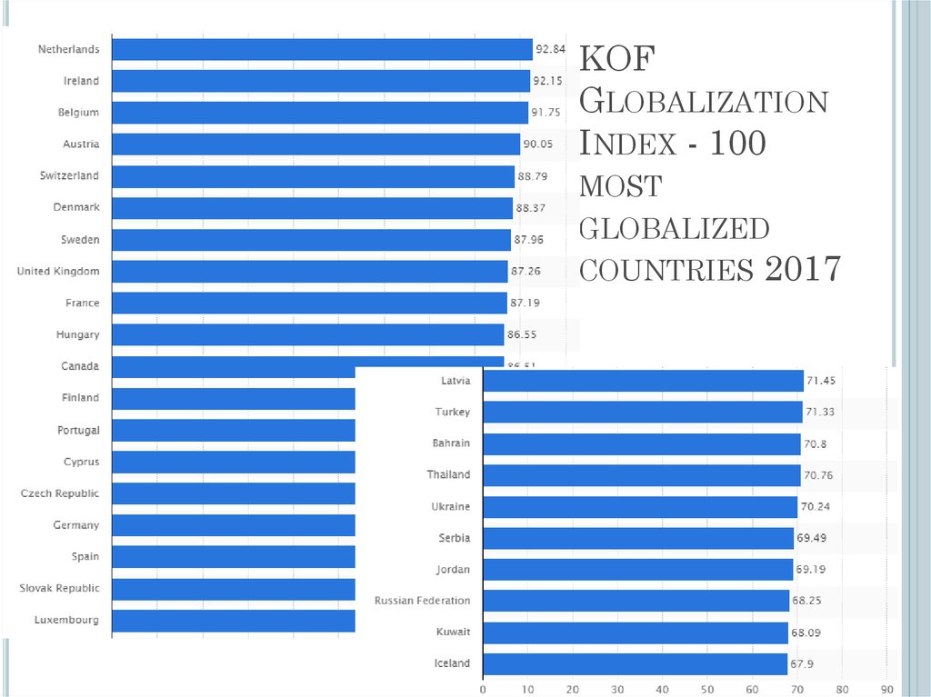
● Konjunkturforschungsstelle (KOF) Swiss Economic
Institute Index of Globalization (2017 – the last data)
124.
THE A. T KEARNEY/FOREIGN POLICYGLOBALIZATION INDEX (UKRAINE 39)
125.
CSGR GLOBALISATION INDEX126.
KOFGLOBALIZATION
INDEX - 100
MOST
GLOBALIZED
COUNTRIES 2017
127.
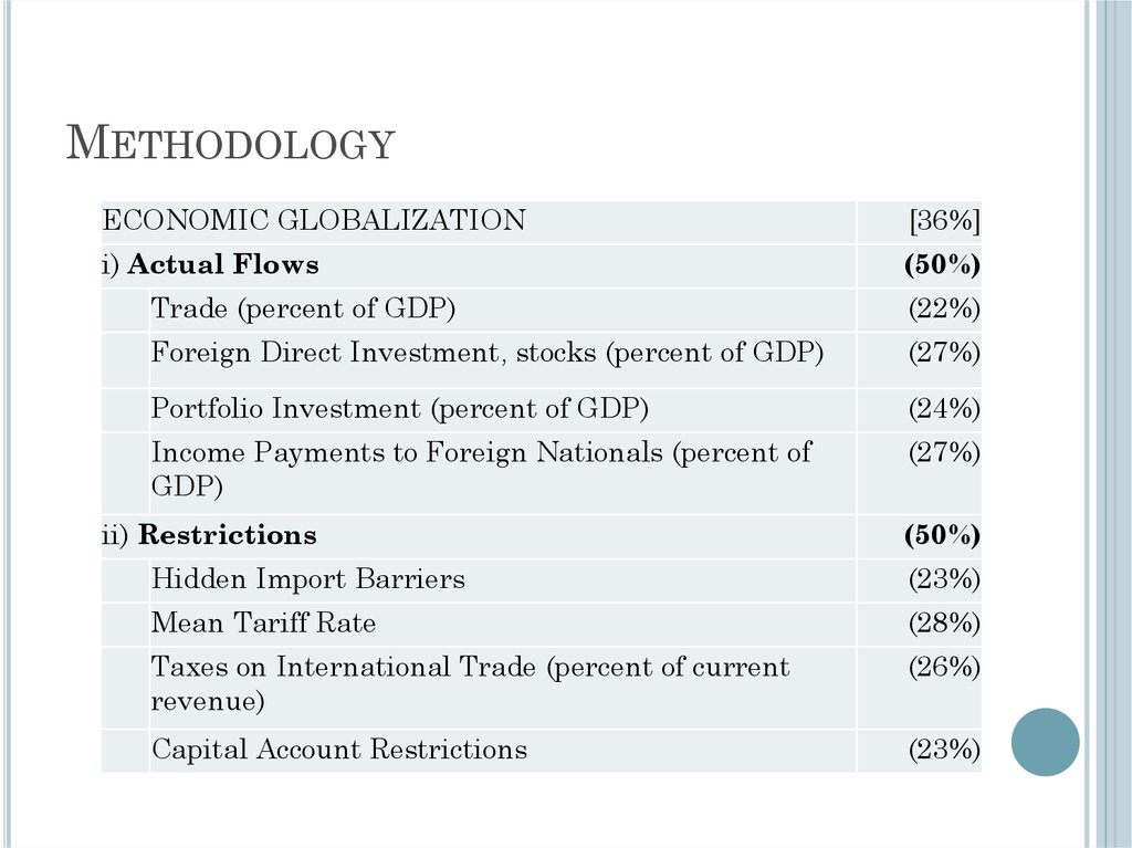
METHODOLOGYECONOMIC GLOBALIZATION
[36%]
i) Actual Flows
(50%)
Trade (percent of GDP)
(22%)
Foreign Direct Investment, stocks (percent of GDP)
(27%)
Portfolio Investment (percent of GDP)
(24%)
Income Payments to Foreign Nationals (percent of
GDP)
(27%)
ii) Restrictions
(50%)
Hidden Import Barriers
(23%)
Mean Tariff Rate
(28%)
Taxes on International Trade (percent of current
revenue)
(26%)
Capital Account Restrictions
(23%)
128.
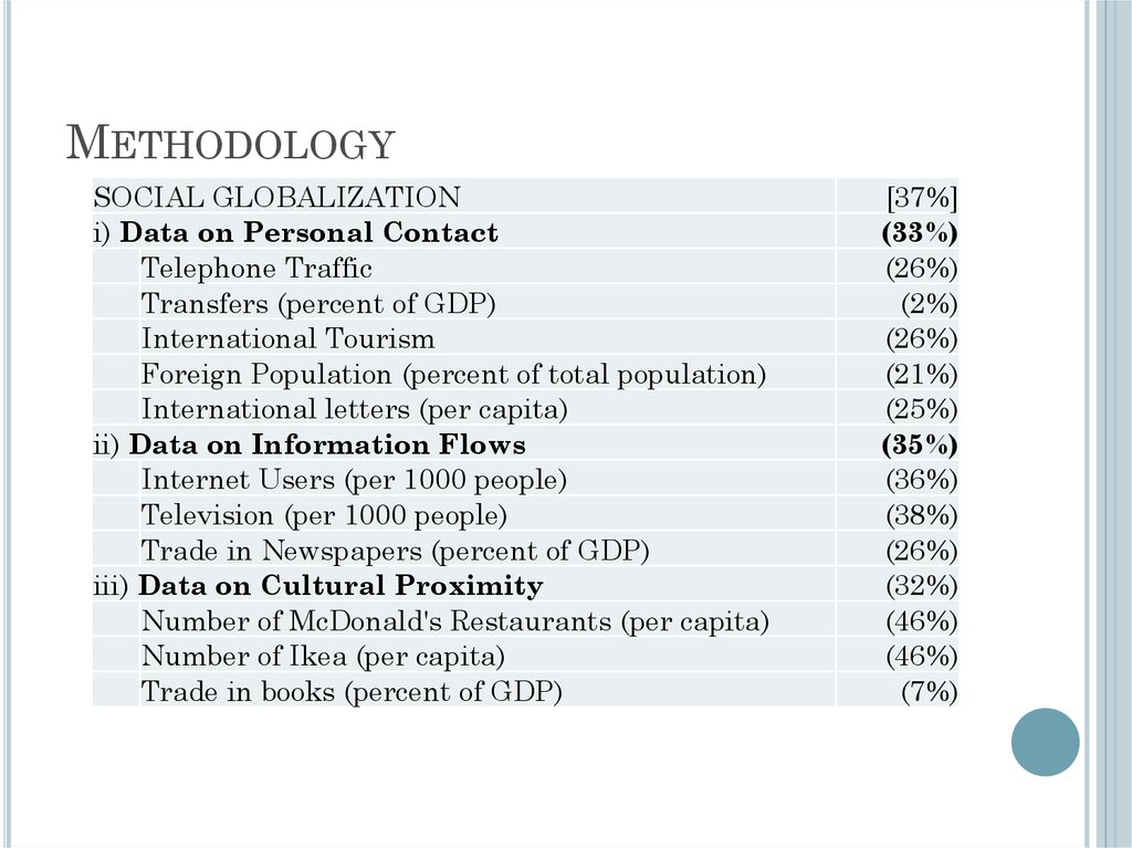
METHODOLOGYSOCIAL GLOBALIZATION
i) Data on Personal Contact
Telephone Traffic
Transfers (percent of GDP)
International Tourism
Foreign Population (percent of total population)
International letters (per capita)
ii) Data on Information Flows
Internet Users (per 1000 people)
Television (per 1000 people)
Trade in Newspapers (percent of GDP)
iii) Data on Cultural Proximity
Number of McDonald's Restaurants (per capita)
Number of Ikea (per capita)
Trade in books (percent of GDP)
[37%]
(33%)
(26%)
(2%)
(26%)
(21%)
(25%)
(35%)
(36%)
(38%)
(26%)
(32%)
(46%)
(46%)
(7%)
129.
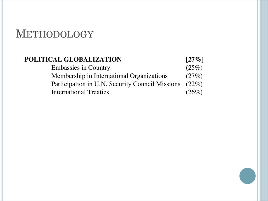
METHODOLOGYPOLITICAL GLOBALIZATION
Embassies in Country
Membership in International Organizations
Participation in U.N. Security Council Missions
International Treaties
[27%]
(25%)
(27%)
(22%)
(26%)
130.
“Arguably no other place onearth has so engineered itself to
prosper from globalization - and
succeeded at it. The small
island nation of 5 million people
boasts the world's secondbusiest seaport, a far higher per
capita income than its former
British overlord and a raft of
No. 1 rankings on lists ranging
from least-corrupt to most
business-friendly countries.”
Singapore a 'canary in the gold
mine of globalization’
Straits Times, May 24 2014
131.
ECONOMIC DIMENSIONGrowing economic interdependence of countries
worldwide through increasing volume and variety
of cross-border transactions in goods and
services, free international capital flows, and
more rapid and widespread diffusion of
technology
132.
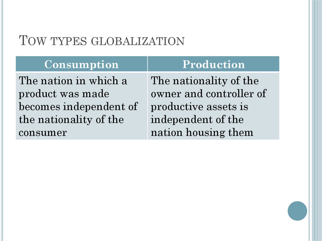
TOW TYPES GLOBALIZATIONConsumption
The nation in which a
product was made
becomes independent of
the nationality of the
consumer
Production
The nationality of the
owner and controller of
productive assets is
independent of the
nation housing them
133.
MEASURING GLOBALIZATION (ECONOMICASPECTS)
Statistics related to trade.
Total exports, total trade (imports + exports),
Trade as a % of GDP
Statistics related to FDI.
Foreign Direct Investment. Money invested in a
country by a foreign company. FDI inflows and
outlflows.
134.
FACTORS WHICH HELP THE SPREAD OFGLOBALISATION
Low transport costs, containerization
Telecommunications
Internet
Low trade barriers
Political stability
Increasing role of TNCs
135.
INCREASED COMPETITION AMONG NATIONSFor example, many companies have shifted their
production facilities to emerging markets such as
China and India to enjoy lower costs of
production.
Benefiting from the increased revenue, these
countries are able to rapidly develop their
infrastructure such as road networks and
industrial parks, which further increased their
attractiveness to foreign investors.
This poses a strong challenge for developed
economies like Singapore and Taiwan and more
so for less developed countries with poor
infrastructure and political stability such as
Cambodia and East Timor
136.
INCREASED COMPETITION AMONG NATIONS“They (economists) predict that increased
competition from low-wage countries will destroy
jobs in richer nations and there will be a “race to
the bottom” as countries reduce wages, taxes,
welfare and environmental controls so as to be
more competitive, at enormous social cost.
Pressure to compete will erode the ability of
governments to set their own economic policies
and the move towards deregulation will reduce
their power to protect and promote the interests
of their people.”
World Health Organization
137.
WIDENING INCOME GAPFor example, with improved communications and
transportation, business owners in developed
countries are able to outsource their operations to
other countries to enjoy lower costs of production.
This inevitably leads to higher retrenchment
rates and loss of income among the average
workers, which translates into the rich getting
richer and the poor becoming poorer
138.
PROS AND CONS OF GLOBALIZATION1. Free trade is supposed to reduce barriers such as tariffs, value
added taxes, subsidies, and other barriers between nations. This
is not true. There are still many barriers to free trade. The
Washington Post story says “the problem is that the big G20
countries added more than 1,200 restrictive export and import
measures since 2008
2. The proponents say globalization represents free trade which
promotes global economic growth; creates jobs, makes companies
more competitive, and lowers prices for consumers.
3. Competition between countries is supposed to drive prices down.
In many cases this is not working because countries manipulate
their currency to get a price advantage.
4. It also provides poor countries, through infusions of foreign
capital and technology, with the chance to develop economically
and by spreading prosperity, creates the conditions in which
democracy and respect for human rights may flourish. This is an
ethereal goal which hasn’t been achieved in most countries
139.
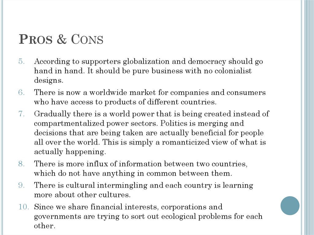
PROS & CONS5.
According to supporters globalization and democracy should go
hand in hand. It should be pure business with no colonialist
designs.
6.
There is now a worldwide market for companies and consumers
who have access to products of different countries.
7.
Gradually there is a world power that is being created instead of
compartmentalized power sectors. Politics is merging and
decisions that are being taken are actually beneficial for people
all over the world. This is simply a romanticized view of what is
actually happening.
8.
There is more influx of information between two countries,
which do not have anything in common between them.
9.
There is cultural intermingling and each country is learning
more about other cultures.
10. Since we share financial interests, corporations and
governments are trying to sort out ecological problems for each
other.
140.
PROS & CONS11. Socially we have become more open and tolerant
towards each other and people who live in the other part
of the world are not considered aliens.
12. Most people see speedy travel, mass communications
and quick dissemination of information through the
Internet as benefits of globalization.
13. Labor can move from country to country to market their
skills. (but this can cause problems with the existing
labor and downward pressure on wages).
14. Sharing technology with developing nations will help
them progress (true for small countries but stealing
technologies and IP have become a big problem with
larger competitors like China).
15. Transnational companies investing in installing plants
in other countries provide employment for the people in
those countries often getting them out of poverty.
16. Globalization has given countries the ability to agree to
free trade agreements like NAFTA, South Korea Korus,
and The TPP.
141.
PROS & CONS1.
2.
3.
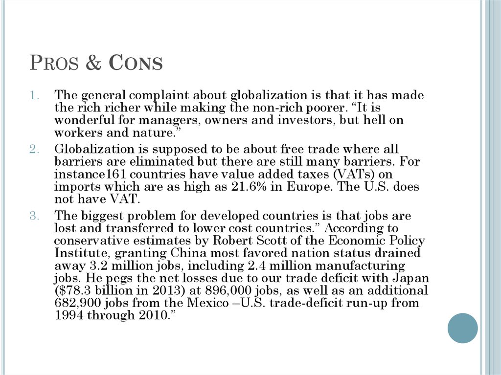
The general complaint about globalization is that it has made
the rich richer while making the non-rich poorer. “It is
wonderful for managers, owners and investors, but hell on
workers and nature.”
Globalization is supposed to be about free trade where all
barriers are eliminated but there are still many barriers. For
instance161 countries have value added taxes (VATs) on
imports which are as high as 21.6% in Europe. The U.S. does
not have VAT.
The biggest problem for developed countries is that jobs are
lost and transferred to lower cost countries.” According to
conservative estimates by Robert Scott of the Economic Policy
Institute, granting China most favored nation status drained
away 3.2 million jobs, including 2.4 million manufacturing
jobs. He pegs the net losses due to our trade deficit with Japan
($78.3 billion in 2013) at 896,000 jobs, as well as an additional
682,900 jobs from the Mexico –U.S. trade-deficit run-up from
1994 through 2010.”
142.
PROS & CONS4.
5.
6.
7.
8.
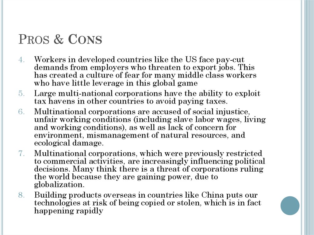
Workers in developed countries like the US face pay-cut
demands from employers who threaten to export jobs. This
has created a culture of fear for many middle class workers
who have little leverage in this global game
Large multi-national corporations have the ability to exploit
tax havens in other countries to avoid paying taxes.
Multinational corporations are accused of social injustice,
unfair working conditions (including slave labor wages, living
and working conditions), as well as lack of concern for
environment, mismanagement of natural resources, and
ecological damage.
Multinational corporations, which were previously restricted
to commercial activities, are increasingly influencing political
decisions. Many think there is a threat of corporations ruling
the world because they are gaining power, due to
globalization.
Building products overseas in countries like China puts our
technologies at risk of being copied or stolen, which is in fact
happening rapidly
143.
PROS & CONSThe anti-globalists also claim that globalization is not
working for the majority of the world. “During the most recent
period of rapid growth in global trade and investment, 1960 to
1998, inequality worsened both internationally and within
countries. The UN Development Program reports that the
richest 20 percent of the world's population consume 86
percent of the world's resources while the poorest 80 percent
consume just 14 percent. “
10. Some experts think that globalization is also leading to the
incursion of communicable diseases. Deadly diseases like
HIV/AIDS are being spread by travelers to the remotest
corners of the globe.
11. Globalization has led to exploitation of labor. Prisoners and
child workers are used to work in inhumane conditions. Safety
standards are ignored to produce cheap goods. There is also
an increase in human trafficking.
12. Social welfare schemes or “safety nets” are under great
pressure in developed countries because of deficits, job losses,
and other economic ramifications of globalization.
9.
144.
DOCUMENTORY145.
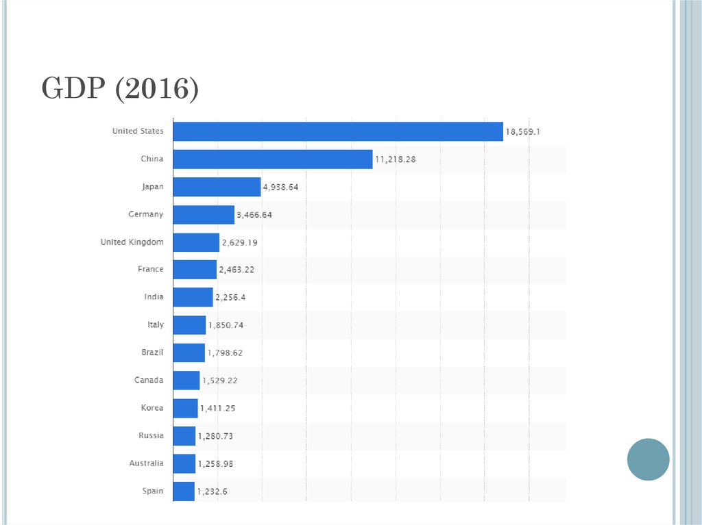
GDP (2016)146.
GDP PER CAPITA (2016)147.
MACROECONOMICSPRODUCTIVITY, OUTPUT &
EMPLOYMENT
Zharova Liubov
Zharova_l@ua.fm
148.
HOW MUCH DOES THE ECONOMY PRODUCE?The quantity that an economy will produce depends on two things
The quantity of inputs utilized in the production process and
The PRODUCTIVITY of the inputs
An economy’s productivity is basic to determining living standards.
In this lecture we shall see how productivity affects people’s incomes
by helping to determine how many workers are employed and how
much they receive.
Among all the inputs for production, labor is usually considered the
most important input.
Therefore, first we shall study the factors that determine demand and
supply of labor and then the forces that bring the labor market into
equilibrium.
Equilibrium in the labor market determines wages and employment;
and the level of employment together with other inputs and the level of
productivity determines how much output en economy produces.
149
149.
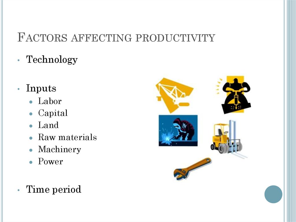
FACTORS AFFECTING PRODUCTIVITYTechnology
Inputs
Labor
● Capital
● Land
● Raw materials
● Machinery
● Power
Time period
150.
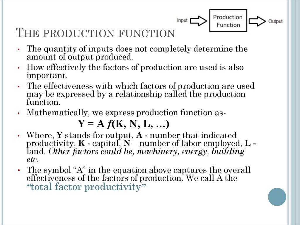
THE PRODUCTION FUNCTIONThe quantity of inputs does not completely determine the
amount of output produced.
How effectively the factors of production are used is also
important.
The effectiveness with which factors of production are used
may be expressed by a relationship called the production
function.
Mathematically, we express production function as-
Y = A f(K, N, L, …)
Where, Y stands for output, A - number that indicated
productivity, K - capital, N – number of labor employed, L land. Other factors could be, machinery, energy, building
etc.
• The symbol “A” in the equation above captures the overall
effectiveness of the factors of production. We call A the
“total factor productivity”
151
151.
EMPIRICAL EXAMPLE: US PRODUCTIONFUNCTION
Studies show that the relationship between outputs
and inputs in the US economy is described reasonably
well by the following production function:
This type of production function is called the CobbDouglas production function.
Historical GDP data of US for the period 1899 – 1922
showed that the production function for US followed
the form:
152
152.
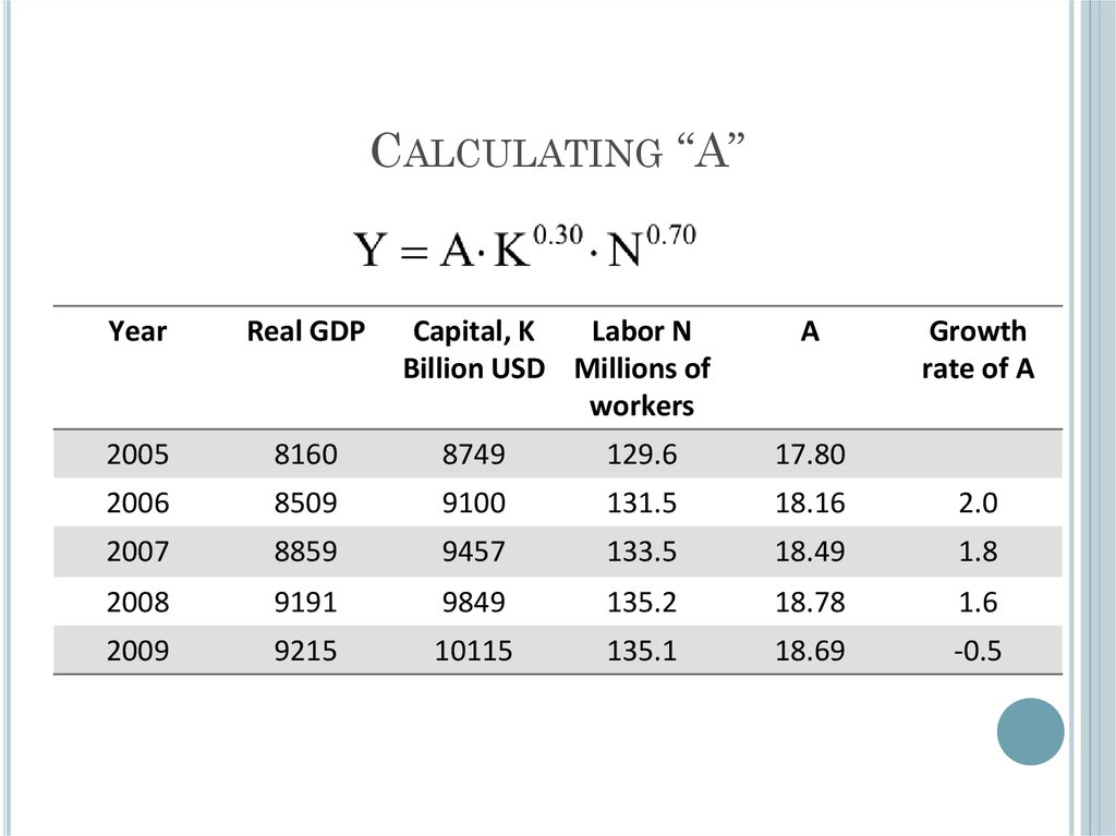
CALCULATING “A”Year
Real GDP
Capital, K
Labor N
Billion USD Millions of
workers
A
Growth
rate of A
2005
8160
8749
129.6
17.80
2006
8509
9100
131.5
18.16
2.0
2007
8859
9457
133.5
18.49
1.8
2008
9191
9849
135.2
18.78
1.6
2009
9215
10115
135.1
18.69
-0.5
153
153.
SHAPE OF THE PRODUCTION FUNCTIONWe can have an idea about the shape of the production
function by holding one of the two factors of production
and the value of total factor productivity (A) constant.
For example, if we want to see the relationship
between capital and total output for the year 2009,
then we hold the values of A and N constant for that
year and treat K as variable.
As a result our production function gets the shape as:
154
154.
SHAPE OF THE PRODUCTION FUNCTIONK
Y
0
500
700
800
900
1000
2000
3000
4000
5000
6000
7000
8000
9000
10115
0
3739
4136
4305
4460
4603
5667
6400
6977
7460
7879
8252
8590
8898
9216
155
155.
SHAPE OF THE PRODUCTION FUNCTION:PROPERTIES
The production function slopes upward from
left to right: this means that as the capital
stock increases more output can be
produced.
The slope of the production function becomes
flatter from left to right: this means that
although more capital always leads to more
output, it does so at a decreasing rate.
156
156.
EFFECT OF INCREASING 1000 UNITS OF CAPITAL EACHTIME
K
Y
Change in Y
for every
1000 units of
K
2000
5667
…
3000
6400
733
4000
6977
577
5000
7460
483
6000
7880
419
7000
8253
373
8000
8590
337
9000
8899
309
10115
9216
317
Marginal Product of Capital:
Marginal product of capital between
K = 2000 and 3000
What is the marginal product of capital
between K = 4000 and 5000? Is it less than
the previous one? What does it mean?
157
157.
MARGINAL PRODUCTIVITYThe previous example shows that marginal
productivity is falling as we increase the amount
of capital
Generally, when amount of labor is high
compared to the amount of capital, marginal
productivity of capital is high. Alternatively,
when amount of labor is low compared to the
amount of capital, marginal productivity of labor
is high
Real life example: Adamjee Jute Mill had
many workers employed against every
single machine. Therefore, productivity
of workers were low as many workers
used to sit idle without a machine to
work with. If we would have increased
number of machines, perhaps, we could
have increased production of jute; and as
a result productivity of workers would
have increased. Unfortunately, we shut
down the mill!
158
158.
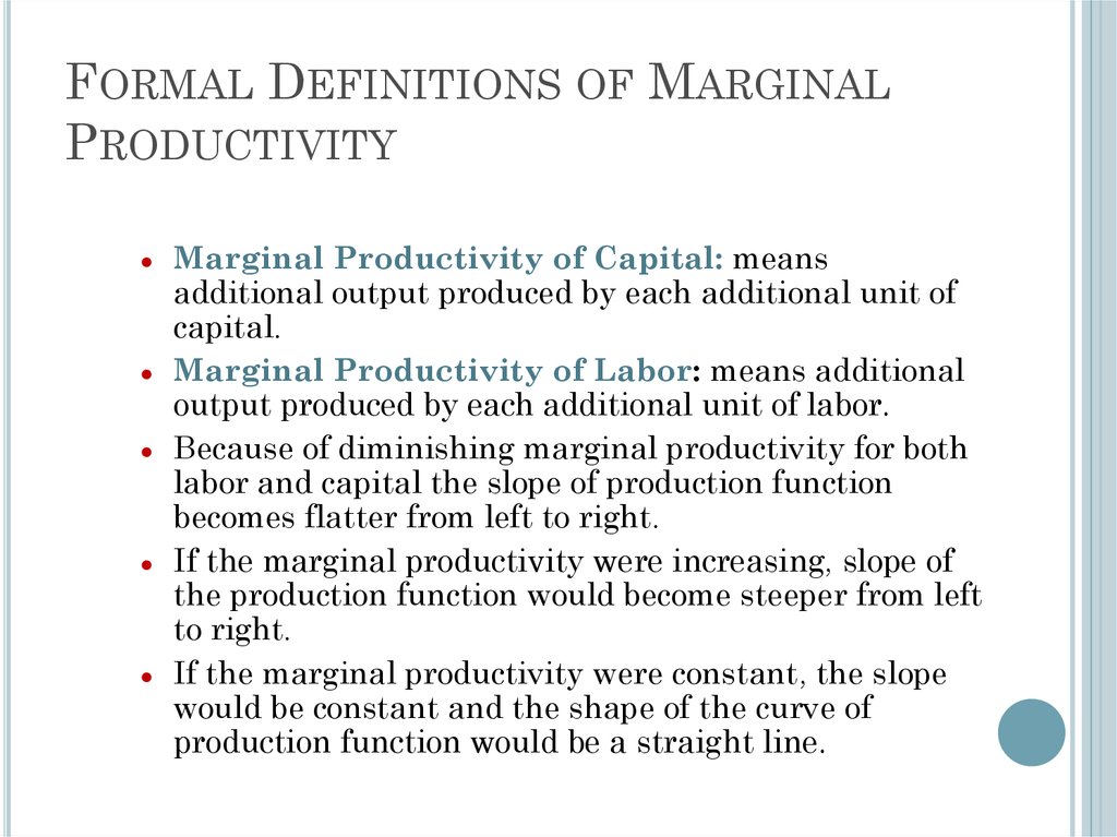
FORMAL DEFINITIONS OF MARGINALPRODUCTIVITY
Marginal Productivity of Capital: means
additional output produced by each additional unit of
capital.
Marginal Productivity of Labor: means additional
output produced by each additional unit of labor.
Because of diminishing marginal productivity for both
labor and capital the slope of production function
becomes flatter from left to right.
If the marginal productivity were increasing, slope of
the production function would become steeper from left
to right.
If the marginal productivity were constant, the slope
would be constant and the shape of the curve of
production function would be a straight line.
159
159.
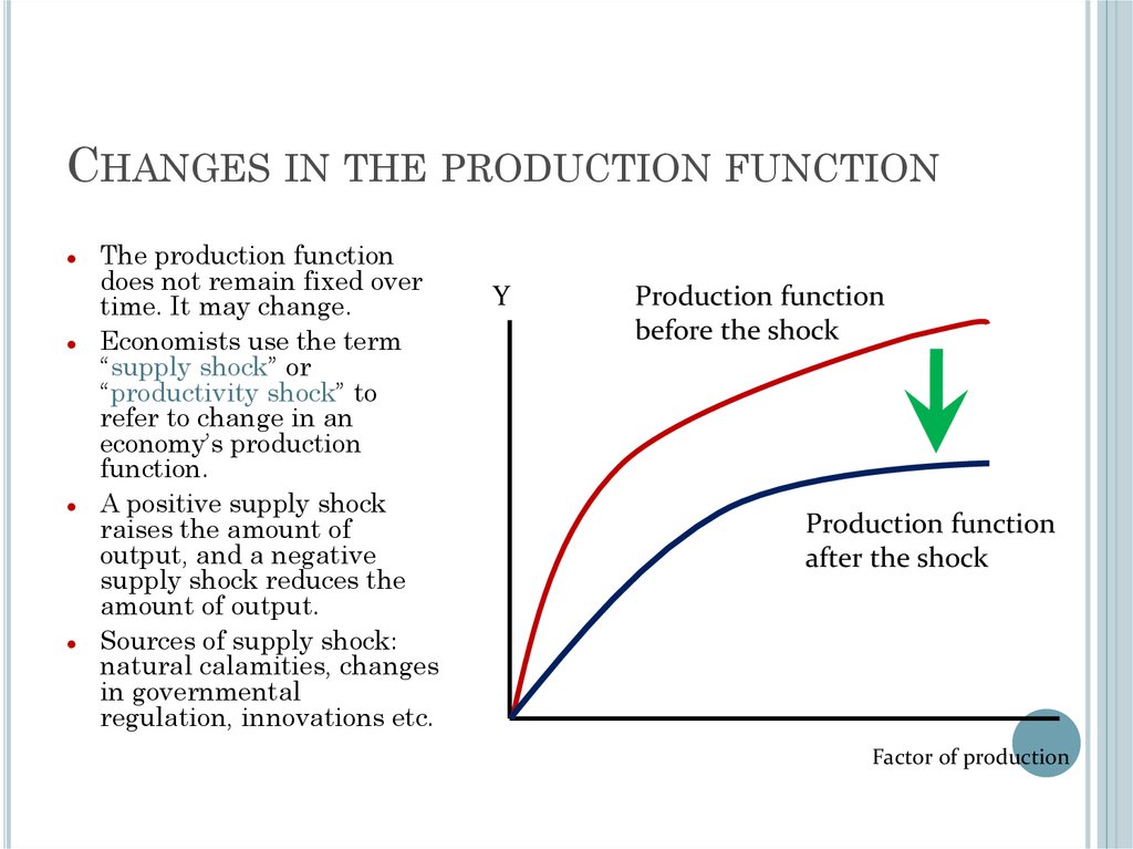
CHANGES IN THE PRODUCTION FUNCTIONThe production function
does not remain fixed over
time. It may change.
Economists use the term
“supply shock” or
“productivity shock” to
refer to change in an
economy’s production
function.
A positive supply shock
raises the amount of
output, and a negative
supply shock reduces the
amount of output.
Sources of supply shock:
natural calamities, changes
in governmental
regulation, innovations etc.
Y
Production function
before the shock
Production function
after the shock
Factor of production
160
160.
DEMAND FOR LABORIn contrast to the amount of capital, the amount of
labor employed in the economy can change quickly.
Thus, year-to-year changes in production can be
traced to the changes in employment.
Demand for labor determines the level of
employment.
For this reason, understanding demand for labor is
important.
To understand demand for labor we shall make the
following assumptions to keep things simple:
Workers are alike
❖ Firms have to pay competitive wage to hire workers
❖ Firms objective is to maximize profit
❖
161
161.
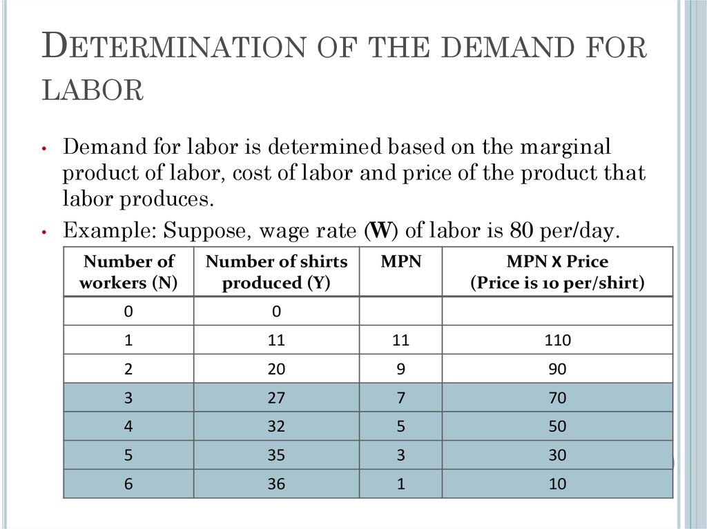
DETERMINATION OF THE DEMAND FORLABOR
Demand for labor is determined based on the marginal
product of labor, cost of labor and price of the product that
labor produces.
Example: Suppose, wage rate (W) of labor is 80 per/day.
Number of
workers (N)
Number of shirts
produced (Y)
MPN
MPN X Price
(Price is 10 per/shirt)
0
0
1
11
11
110
2
20
9
90
3
27
7
70
4
32
5
50
5
35
3
30
6
36
1
10
162
162.
DETERMINATION OF DEMAND FOR LABORTo maximize profit the firm will follow the
following rules:
Increase employment if
for an additional
worker
>
(MPN * price)
W
or
MPN > W/price
Decrease employment if
for an additional
worker
<
(MPN *price)
W
or
MPN < W/price
The expression “W/price” is called, in economics, “real wage”.
Why?
Because when we divide wage by price we get a figure that shows
the units of physical goods produced by labor.
163
163.
DETERMINATION OF LABOR DEMANDThe MPN curve on the
right can be thought of as MPN and real wage
the demand for labor.
Because quantity of labor
is determined by the price
of labor (the real wage).
What happens when the
MPN > w*? Firms hire
more labor.
What happens when MPN
< w*? Firms lay-off labor
What happens at point A?
Equilibrium established.
w*
A
Real wage
MPN
N*
Labor
164
164.
FACTORS THAT SHIFT LABOR DEMANDCURVE
Changes in the wage do not shift the labor
demand curve. Changes in the wage will cause
movement along the labor demand curve.
Factors that shift labor demand curve would be
something that will change the demand for labor
at any given wage.
A beneficial shock will shift the labor demand
curve to the right.
An adverse shock will shift the labor demand
curve to the left.
165
165.
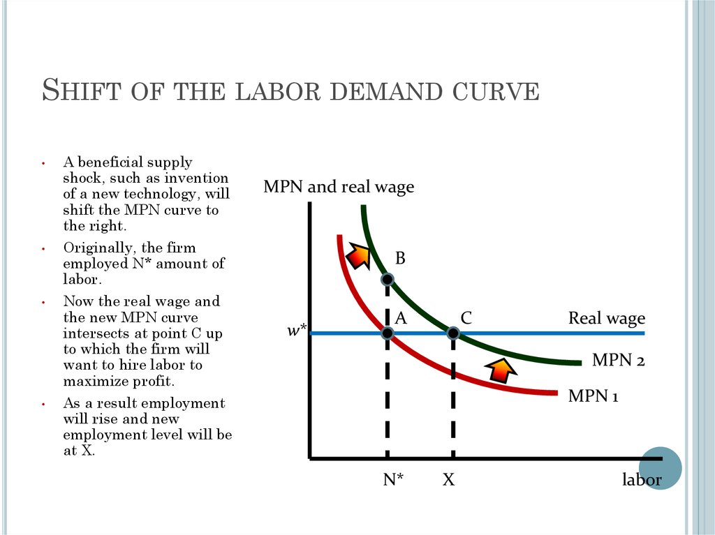
SHIFT OF THE LABOR DEMAND CURVEA beneficial supply
shock, such as invention
of a new technology, will
shift the MPN curve to
the right.
Originally, the firm
employed N* amount of
labor.
Now the real wage and
the new MPN curve
intersects at point C up
to which the firm will
want to hire labor to
maximize profit.
As a result employment
will rise and new
employment level will be
at X.
MPN and real wage
B
w*
A
C
Real wage
MPN 2
MPN 1
N*
X
labor
166
166.
SUPPLY OF LABORWe have seen that firm’s demand for labor depend
on labor productivity and wage paid to labor.
However, supply of labor depends on workers’
personal choice to work.
Personal choice about being a part of the labor
force generally depends on the following two
factors:
Income-leisure trade-off
❖ Real wage
❖
167
167.
LABOR SUPPLY CURVELabor supply curve looks the same as the
supply curve we studied before.
• Usually, we assume that a higher real wage
will increase labor supply.
• Labor supply curve will not shift because of a
change in the wage.
• Any factor that changes the amount of labor
supply at a given wage rate will shift the
labor supply curve.
168
168.
FACTORS THAT SHIFT THE LABORSUPPLY CURVE
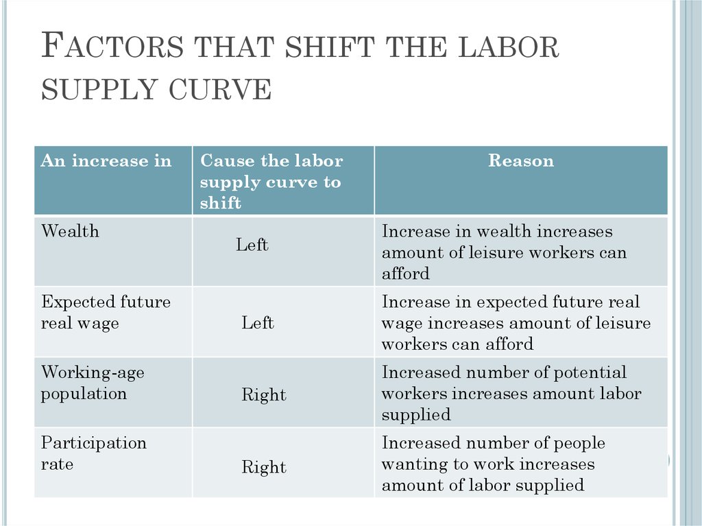
An increase in
Wealth
Expected future
real wage
Working-age
population
Participation
rate
Cause the labor
supply curve to
shift
Left
Reason
Increase in wealth increases
amount of leisure workers can
afford
Left
Increase in expected future real
wage increases amount of leisure
workers can afford
Right
Increased number of potential
workers increases amount labor
supplied
Right
Increased number of people
wanting to work increases
amount of labor supplied
169
169.
LABOR MARKET EQUILIBRIUMMPN and real wage
Labor supply
w*
A
Real wage
MPN/demand for
labor
labor
170
170.
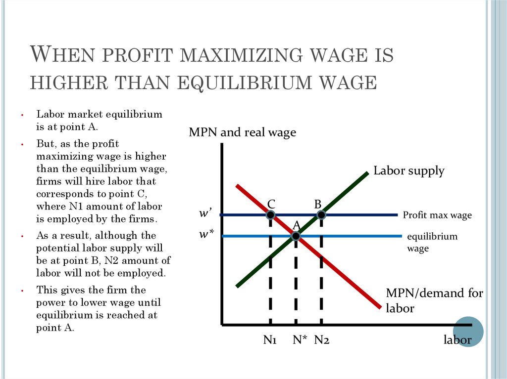
WHEN PROFIT MAXIMIZING WAGE ISHIGHER THAN EQUILIBRIUM WAGE
Labor market equilibrium
is at point A.
But, as the profit
maximizing wage is higher
than the equilibrium wage,
firms will hire labor that
corresponds to point C,
where N1 amount of labor
is employed by the firms.
As a result, although the
potential labor supply will
be at point B, N2 amount of
labor will not be employed.
MPN and real wage
Labor supply
w’
C
B
A
w*
This gives the firm the
power to lower wage until
equilibrium is reached at
point A.
Profit max wage
equilibrium
wage
MPN/demand for
labor
N1
N* N2
labor
171
171.
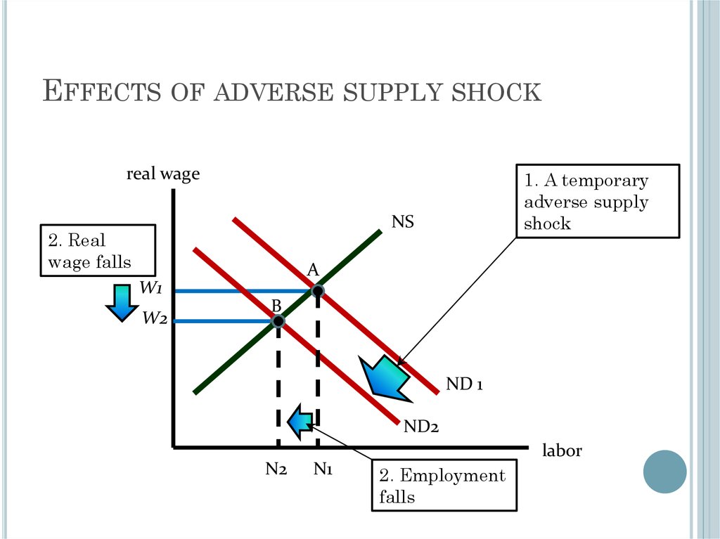
EFFECTS OF ADVERSE SUPPLY SHOCKreal wage
1. A temporary
adverse supply
shock
NS
2. Real
wage falls
A
W1
W2
B
ND 1
ND2
N2
N1
labor
2. Employment
falls
172
172.
WHAT IF ALL WORKERS ARE NOT ALIKE?We assumed that all workers are alike. By this, we meant
that all workers have the same skill level.
However, if workers have different skill level then supply
shocks will not affect all workers in the same way.
Example: if a production process introduces computer
based production, then workers who can operate
computers will cope with the new process quickly. On the
other hand, workers who cannot operate computers will
find it difficult to cope with the process. This will create
difference in the marginal productivity level of these two
groups of workers. Most likely, the workers who can use
computers will get higher wage at cost of those who
cannot.
Therefore, whether a shock will be considered beneficial
or adverse depends on the skill/education level of the
workers.
173
173.
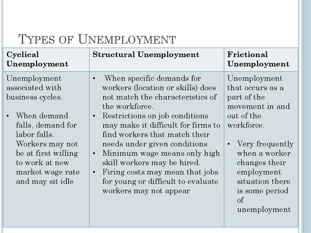
UNEMPLOYMENT: THE UNTOLD STORY OF FULLEMPLOYMENT• Full-employment level implies that all the workers who are
willing to work at the equilibrium wage rate will find a job.
• All workers in real life do not find jobs even if they want to.
When workers are unemployed for a long time the sum of
all such workers constitute “structural unemployment”.
• If workers are unemployed for a brief period (for example:
the brief period in which they search for a suitable job) we
call it “frictional unemployment”.
• The rate of unemployment that prevails when output and
unemployment rate the full-employment level, we call it
natural rate of unemployment.
• The difference between actual unemployment rate and
natural unemployment rate is called cyclical
unemployment.
• If workers are not willing to work, this will not constitute
unemployment. We shall consider these workers as out of
work force.
174
174.
Productivity / GDPper capita & GDP
(PPP)
Prof. Zharova Liubov
Zharova_l@ua.fm
175.
GDP Per Capita / GDP PPP(purchasing parity power)
GDP per capita = GDP / Population (number of
people in the country)
• The per capita GDP is especially useful when
comparing one country to another, because it
shows the relative performance of the countries.
A rise in per capita GDP signals growth in the
economy and tends to reflect an increase in
productivity.
176.
Why do we need GDP percapita?
• sometimes used as an indicator of
standard of living, with higher per capita
GDP equating to a higher standard of
living.
NB: A standard of living is the level of wealth,
comfort, material goods and necessities available to
a certain socioeconomic class or a certain
geographic area. The standard of living includes
factors such as income, gross domestic product,
national economic growth, economic and political
stability,
political
and
religious
freedom,
environmental quality, climate, and safety. The
standard of living is closely related to quality of life.
177.
GDP(2016)
GDP per capita
(2016)
178.
Why do we need GDP percapita?
• can also be used to measure the
productivity of a country's workforce,
as it measures the total output of
goods and services per each member
of the workforce in a given nation.
(better measure of worker productivity may be GDP per
hours worked (?) - per capita GDP does not take into
account the influence of technology over a worker's
output. If two countries each have a workforce that
possesses an equal measure of per capita GDP, it appears
that both nations hold an equal standard of living.
However, a further examination of GDP per hours worked
offers a different view of worker efficiency. The country with
the lower GDP per hours worked actually enjoys more
leisure time.)
Methodology: Productivity is calculated by
dividing each country's GDP by the average
179.
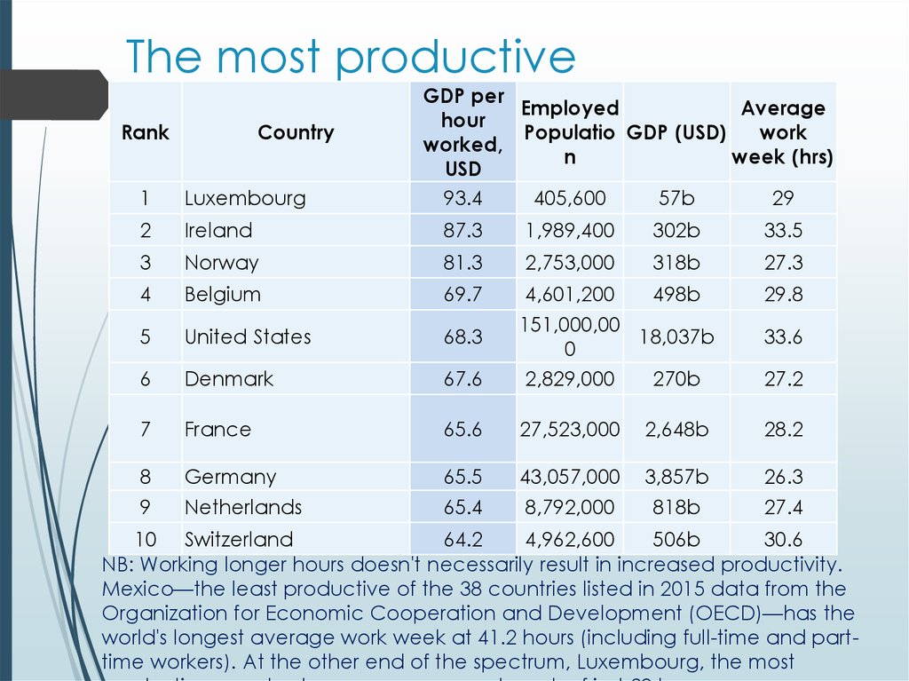
The most productiveGDP per
Employed
Average
hour
countries
(2015)
Rank
Country
Populatio GDP (USD)
work
worked,
USD
93.4
405,600
57b
29
n
week (hrs)
1
Luxembourg
2
Ireland
87.3
1,989,400
302b
33.5
3
Norway
81.3
2,753,000
318b
27.3
4
Belgium
69.7
29.8
5
United States
68.3
6
Denmark
67.6
4,601,200
498b
151,000,00
18,037b
0
2,829,000
270b
7
France
65.6
27,523,000
2,648b
28.2
8
9
Germany
Netherlands
65.5
65.4
43,057,000
8,792,000
3,857b
818b
26.3
27.4
33.6
27.2
10 Switzerland
64.2
4,962,600
506b
30.6
NB: Working longer hours doesn't necessarily result in increased productivity.
Mexico—the least productive of the 38 countries listed in 2015 data from the
Organization for Economic Cooperation and Development (OECD)—has the
world's longest average work week at 41.2 hours (including full-time and parttime workers). At the other end of the spectrum, Luxembourg, the most
180.
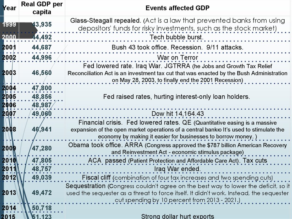
YearReal GDP per
capita
1999
43,935
2000
44,492
Glass-Steagall repealed. (Act is a law that prevented banks from using
depositors' funds for risky investments, such as the stock market)
Tech bubble burst.
2001
44,687
Bush 43 took office. Recession. 9/11 attacks.
2002
44,996
War on Terror
Fed lowered rate. Iraq War. JGTRRA (he Jobs and Growth Tax Relief
2003
46,560
Reconciliation Act is an investment tax cut that was enacted by the Bush Administration
on May 28, 2003, to finally end the 2001 Recession)
2004
2005
2006
2007
47,800
48,856
48,987
49,060
2008
46,941
2009
47,280
2010
2011
2012
47,805
48,757
49,039
2013
49,472
2014
2015
50,718
51,123
Events affected GDP
Fed raised rates, hurting interest-only loan holders.
Dow hit 14,164.43
Financial crisis. Fed lowered rates. QE (Quantitative easing is a massive
expansion of the open market operations of a central bankю It’s used to stimulate the
economy by making it easier for businesses to borrow money. )
Obama took office. ARRA (Congress approved the $787 billion American Recovery
and Reinvestment Act - economic stimulus package)
ACA passed (Patient Protection and Affordable Care Act). Tax cuts
Iraq War ended.
Fiscal cliff (combination of four tax increases and two spending cuts)
Sequestration (Congress couldn't agree on the best way to lower the deficit, so it
used the sequester as a threat to force itself. It didn't work. Instead, the sequester
cut spending by 10 percent from 2013 - 2021.)
Strong dollar hurt exports
181.
Labour productivity• Labour productivity is defined as real gross
domestic product (GDP) per hour worked.
This captures the use of labour inputs better than just
output per employee, with labour input defined as
total hours worked by all persons involved.
The data are derived as average hours worked
multiplied by the corresponding and consistent
measure of employment for each particular country.
Forecast is based on an assessment of the economic
climate in individual countries and the world
economy, using a combination of model-based
analyses and expert judgement. This indicator is
measured as an index with 2010=1.
182.
183.
Labour productivity andutilization
• Labour productivity growth is a key dimension of
economic performance and an essential driver of
changes in living standards. Growth in gross
domestic product (GDP) per capita can be
broken down into growth in labour productivity,
measured as growth in GDP per hour worked,
and changes in the extent of labour utilisation,
measured as changes in hours worked per
capita. High labour productivity growth can
reflect greater use of capital, and/or a decrease
in the employment of low-productivity workers, or
general efficiency gains and innovation
184.
185.
Multifactor productivity• Multifactor productivity (MFP) reflects the overall
efficiency with which labour and capital inputs
are used together in the production process.
Changes in MFP reflect the effects of changes in
management practices, brand names,
organizational change, general knowledge,
network effects, spillovers from production factors,
adjustment costs, economies of scale, the effects
of imperfect competition and measurement
errors.
• Growth in MFP is measured as a residual, i.e. that
part of GDP growth that cannot be explained by
changes in labour and capital inputs. In simple
terms therefore, if labour and capital inputs
remained unchanged between two periods, any
changes in output would reflect changes in MFP.
This indicator is measured as an index and in annual
186.
187.
What Is Purchasing PowerParity?
Macroeconomic analysis relies on several different
metrics to compare economic productivity and
standards of living between countries and across time.
One popular metric is purchasing power parity (PPP).
Purchasing Power Parity (PPP) is an economic theory
that compares different countries' currencies through a
market "basket of goods" approach. According to this
concept, two currencies are in equilibrium or at par
when a market basket of goods (taking into account
Where:
the exchange
rate) is priced the same in both
countries. S represents exchange rate of currency 1
to currency 2
P1 represents the cost of good "x" in
currency 1
P2 represents the cost of good "x" in
currency
188.
PPP calculationProblem: To make a comparison of prices across countries that
holds any type of meaning, a wide range of goods and
services must be considered. The amount of data that must be
collected, and the complexity of drawing comparisons makes
this process difficult.
Solution: To facilitate this, the International Comparisons
Program (ICP) (established in 1968 by the University of
Pennsylvania and UN). Purchasing power parities generated by
the ICP are based on a worldwide price survey that compares
the prices of hundreds of various goods. This data, in turn, helps
international macroeconomists come up with estimates of
global productivity and growth.
Correction & Updating: Every three years, the World Bank
constructs and releases a report that compares various
countries in terms of PPP and U.S. dollars.
Usage: Both the International Monetary Fund (IMF) and the
Organization for Economic Cooperation and Development
(OECD) use weights based on PPP metrics to make predictions
and recommend economic policy.
189.
The Big Mac Index: an exampleof PPP
(The Economist)
Prehistory:
The Economist has tracked the price of
McDonald's Corp.’s (MCD) Big Mac burger in many
countries since 1986.The highly publicized Big Mac Index is
used to measure the purchasing power parity (PPP)
between nations, using the price of a Big Mac as the
benchmark. The Big Mac index suggests that, in theory,
changes in exchange rates between currencies should
affect the price that consumers pay for a Big Mac in a
particular nation, replacing the "basket" with the famous
hamburger.
Example: if the price of a Big Mac is $4.00 in the U.S. as
compared to 2.5 pounds sterling in Britain, we would
expect that the exchange rate would be 1.60 (4/2.5 =
1.60). If the exchange rate of dollars to pounds is any
greater, the Big Mac Index would state that the pound
was overvalued, any lower and it would be under-valued.
Flaws: (1) the Big Mac's price is decided by McDonald's
190.
191.
GDP with PPPExample: One way to think of what GDP with PPP
represents is to imagine the total collective purchasing
power of Japan if it were used to make the same
purchases in U.S. markets. This only works after all yen are
exchanged for dollars, otherwise, the comparison does
not make sense. The net effect is to describe how many
dollars it takes to buy $1 worth of goods in Japan as
opposed to in the U.S.
GDP at PPP reflects the purchasing power of a citizen in
one country to a citizen of another.
BUT (!) empirical evidence has shown that for many goods
and baskets of goods, PPP is not observed in the short“Burgernomics”
by Michael over
Pakko
and Patricia
term,
and there is uncertainty
whether
it applies in
Pollard
(2003) explores the Big Mac Index and PPP
the
long-term
and cites several confounding factors as to why
PPP theory does not line up with reality.
192.
Transport Costs: Goods that are not available locally will
need to be imported, resulting in transport costs.
Imported goods will consequently sell at a relatively
higher price than the same goods available from local
sources.
Taxes: When government sales taxes, such as valueadded tax (VAT), are high in one country relative to
another, this means goods will sell at a relatively higher
price in the high-tax country.
Government Intervention: Import tariffs add to the price
of imported goods. Where these are used to restrict
supply, demand rises, causing the price of the goods to
rise as well. In countries where the same good is
unrestricted and abundant, its price will be lower.
Governments that restrict exports will see a good's price
rise in importing countries facing a shortage, and fall in
exporting countries where its supply is increasing.
Non-Traded Services: those costs are unlikely to be at
parity internationally. These costs can include the cost of
the storefront, and other expenses such as insurance,
heating and the cost of labor.
Market Competition: Goods might be deliberately priced
193.
Venezuela case194.
From the 10 years of military dictatorship between 19481958 to the impeachment of Carlos Andrés Pérez for
corruption in 1993, Venezuelan politics have often
been both rocky and eventful.
But despite these challenges throughout its history, no
one has ever denied Venezuela’s economic potential.
After the discovery of oil in the early 20th century, the
nation quickly built its economy on back of black gold
– and even today, Venezuela leads the world in
proven oil reserves with 300 billion barrels.
195.
By 1950, as the rest of the world was struggling to recoverfrom World War II, Venezuela had the fourth-richest GDP
per capita on Earth. The country was 2x richer than Chile, 4x
richer than Japan, and 12x richer than China!
Unfortunately for Venezuela, this wealth wouldn’t last –
and an over-reliance on oil would soon decimate the
economy in unexpected ways.
196.
The Downfall of Venezuela’sEconomy
From 1950 to the early 1980s, the Venezuelan economy
experienced steady growth.
By 1982, Venezuela was still the richest major economy in
Latin America. The country used its vast oil wealth to pay
for social programs, including health care, education,
transport, and food subsidies. Workers in Venezuela were
among the highest paid in the region.
However, from there things went quickly downhill. In the
mid-1980s, an oil glut and a free-falling oil price ended up
decimating the Venezuelan economy, which was unable
to diversify away from energy.
Today, Venezuela has one of the poorest major
economies in Latin America – and as the current crisis
rides itself out, the IMF foresees it getting far worse. By
2022, the organization predicts Venezuela’s GDP per
capita (PPP) will be just $12,210, which would be a
197.
198.
• Although oil revenues are tempting to rely on tomaintain social order, they come with a degree
of unpredictability. According to OPEC,
Venezuela still relies on oil for 95% of its exports,
which means that any fluctuations in oil price can
be the difference between immense wealth and
near-poverty.
• After the oil glut in the 1980s, Venezuela’s oil
revenues dropped significantly. It was then that
Venezuela had its first bout with inflation, where
rates peaked in 1989 (84.5% inflation) and later in
1996 (99.9% inflation). Without sufficient money
coming in, the country had to rely on its printing
presses in an attempt to maintain living standards
• In 1998, Hugo Chávez was elected with the
promise that Venezuela could reduce poverty
and step up living standards by leaning even
199.
The graphicshows
Venezuela’s
oil revenues
(in 2000
dollars)
against the
rate of
inflation – and
it symbolizes
the story of
Venezuela’s
recent
economic
history as
succinctly as
possible.
200.
Nicolás Maduro, who took over after the death of his
predecessor, saw oil prices crash almost immediately,
and it was clear that Venezuela’s intense battle with
inflation was only just beginning. The national currency,
the Venezuelan bolívar, would soon be almost
worthless.
201.
• The details of today’s crisis and intensehyperinflation are widely shared.
(http://money.visualcapitalist.com/trajectoryvenezuelan-hyperinflation-familiar/)
• The country has massive shortages of food,
electricity, and other essential goods, and
violence is escalating in Caracas. More recently,
the government is attempting to tighten its grip
around power, and mismanagement of the
economy has led to people starving on the
streets. People are calling the situation a
humanitarian crisis, which is extremely
disheartening to see in what was once one of the
richest countries on the planet.
• And while the current condition of Venezuela is a
202.
MACROECONOMICSCONSUMPTION, SAVINGS
& INVESTMENT
Zharova Liubov
Zharova_l@ua.fm
203.
CONSUMPTIONConsumption can be defined in different ways,
but is usually best described as the final
purchase of goods and services by individuals. It
is also often referred to as consumer spending
Every time you purchase food at the drive-thru or
pull out your debit or credit card or cash to buy
something, you are adding to consumption.
Consumption is one of the biggest concepts in
economics and is extremely important because it
helps determine the growth and success of the
economy.
Businesses can open up and offer all kinds of great
products, but if we don't purchase or consume their
products, they won't stay in business very long
204.
THEORIES OF CONSUMPTIONKeynes mentioned several subjective and
objective factors which determine consumption of
a society. However, according to Keynes, of all
the factors it is the current level of income that
determines the consumption of an individual and
also of society.
● Since Keynes lays stress on the absolute size of
income as a determinant of consumption, his theory
of consumption is also known as absolute income
theory.
● Keynes put forward a psychological law of
consumption, according to which, as income increases
consumption increases but not by as much as the
increase in income. In other words, marginal
propensity to consume is less than one.
205.
S. KUZNETS VISIONContrary to Keynes’s proposition that proportion of income
spent on consumption declines as income increases (that is,
average propensity to consume falls with the increase in
income), Kuznets found from a statistical empirical study of
consumption of the economy of the USA that average
propensity to consume had remained constant over a long
period despite the substantial increase in income.
How the average propensity to consume has remained
stable despite the substantial increase in income has been
a great puzzle in consumption theory for a long time.
206.
Theories of ConsumptionRelative Income
Theory of
Consumption
• consumption
expenditure depends
on income of an
individual relative to
incomes of others
rather than the
absolute size of his
own income
Life Cycle Theory Permanent
of Consumption
Income Theory of
Consumption
• individual plans his
even consumption
profile in his lifetime
which depends not so
much on his current
income but on his
expectations of
income in the whole
lifetime
• consumption of an
individual depends
on permanent income
rather than current
level of income
207.
RELATIVE INCOME THEORY OFCONSUMPTION (J.S. DUESENBERRY)
Assumptions:
the determinant of consumption is relative income of
an individual rather than his absolute income
● the consumption of a person does not depend on his
current income but on certain previously reached
income level
because his relative income has remained the same the
individual will spend the same proportion of his
income on consumption as he was doing before the
absolute increase in his income. That is, his average
propensity to consume (APC) will remain the
same despite the increase in his absolute income.
208.
Demonstration Effect: individuals or
households try to imitate or copy the
consumption levels of their neighbours or other
families in a particular community. This is called
demonstration effect or Duesenberry effect.
if incomes of all families increase in
the same proportion, distribution of
relative incomes would remain
unchanged and therefore the
proportion of consumption expenditure
to income which depends on relative
income will remain constant.
family with a given income would
devote more of his income to
consumption if it is living in a
community in which that income is
regarded as relatively low because
of the working of demonstration
effect.
209.
Ratchet Effect - when income of individuals or
households falls, their consumption expenditure
does not fall much
this is partly due to the demonstration effect. People do not
want to show to their neighbours that they no longer afford to
maintain their high standard of living.
partly due to the fact that they become accustomed to their
previous higher level of consumption and it is quite hard and
difficult to reduce their consumption expenditure when their
income has fallen. They maintain their earlier consumption
level by reducing their savings. Therefore, the fall in their
income, as during the period of recession or depression, does
not result in decrease in consumption expenditure very much
as one would conclude from family budget studies.
210.
LIFE CYCLE THEORY OF CONSUMPTION( ALBERT ANDO & FRANCO MODIGLIANI)
Idea: the consumption in any period is not the
function of current income of that period but of
the whole lifetime expected income
Assumptions:
to plan a pattern of consumption expenditure based
on expected income in their entire lifetime
● individual maintains a more or less constant or
slightly increasing level of consumption
● his level of consumption is limited by his expectations
of lifetime income
211.
A typical individual in this theory in his early years of life spends
on consumption either by borrowing from others or spending the
assets bequeathed from his parents.
It is in his main working years of his lifetime that he consumes less
than the income he earns and therefore makes net positive savings.
He invests these savings in assets, that is, accumulates wealth
which he consumes in the future years. In his lifetime after
retirement he again dissaves, that is, consumes more than his
income in these later years of his life but is able to maintain or even
slightly increase his consumption in the lifetime after retirement.
212.
Shortcomings:
criticized the assumption of life cycle hypothesis that
in making consumption plans, households have “a
definite and conscious vision.”
● theory fails to recognize the importance of liquidity
constraints in determining the response of
consumption to income. According to critics, even if a
household has a concrete vision of future income, the
opportunities to borrow from the capital markets for
quite a long period on the basis of expected future
income are very little.
213.
PERMANENT INCOME THEORY OFCONSUMPTION (MILTON FRIEDMAN)
Assumptions:
consumption is determined by long-term expected
income (permanent income) rather than current
level of income (According to Friedman, an individual who
is paid or receives income only once a week, say on Friday, he
would not concentrate his consumption on one day with zero
consumption on all other days of the week)
an individual would prefer a smooth consumption
flow per day rather than plenty of consumption today
and little consumption tomorrow. Thus consumption
in one day is not determined by income received on
that particular day.
● permanent income or expected long-term average
income is earned from both “human and non-human
wealth”
214.
Relationship between Consumption andPermanent Income: Cp = k(i,w,u) ×Yp
Cp – permanent consumption;
Yp – permanent income
k - the proportion of permanent income that is
consumed
➢
➢
➢
Rate of interest (i): at a higher rate of interest the
people would tend to save more and their consumption
expenditure will decrease.
The proportion of non-human wealth to human
wealth (w): the greater the amount of wealth or assets
held by an individual, the greater would be its
propensity to consume and vice-versa
Desire to add to one’s wealth (u): households’
preference for immediate consumption as against the
desire to add to the stock of wealth or assets also
determines the proportion of permanent income to be
devoted to consumption
215.
In addition to permanent income (Yp), the
individual’s income may contain a transitory
component - transitory income (Yt). A
transitory income is a temporary income that is
not going to persist in future periods.
When income of an individual increases in the current year as
compared to the last year, the permanent income will be less than
the current year’s income. This is because individual is not sure
whether the increase in income will persist in the future and
therefore does not immediately revise his estimate of permanent
income by the full amount of the increase in his income in the
current year
216.
Conclusions:
Permanent income hypothesis is similar to life cycle
hypothesis and differs only in details
Permanent income hypothesis is also consistent with
the evidence from the cross-sectional budget studies
that high income families have low average
propensity to consume than that of low- income
families. A sample of high income families at a given
time is likely to contain a relatively larger number of
families who are having positive transitory increase
in incomes.
laying stress on changes in rate of interest and the
wealth or assets held by the people and desire to add
to one’s wealth as important determinants of
consumption and savings, Friedman’s permanent
income hypothesis has made an important
contribution to the theory of consumption and saving.
217.
REAL INCOME VS. NOMINAL INCOMEThe term 'real' that is used in describing income
refers to how your income is affected by
inflation, or the natural rise in prices of goods
and services. So to elaborate, if your income went
up 5% in a year, but the price of goods or
inflation went up 5% also, your real income
remained flat. You can't really buy or consume
any more goods than you could before.
218.
SAVINGSSavings, according to Keynesian economics, consists of the amount
left over when the cost of a person's consumer expenditure is
subtracted from the amount of disposable income he earns in a
given period of time. For those who are financially prudent, the
amount of money left over after personal expenses have been met
can be positive; for those who tend to rely on credit and loans to
make ends meet, there is no money left for savings.
Saving involves income that is not consumed
Savings can be turned into further increased income
through investing in different investment vehicles.
Saving is often confused with investing, but they are not the
same.
● Although most people think of purchases of stocks and BONDS
as investments, economists use the term “INVESTMENT” to
mean additions to the real stock of capital: plants, factories,
equipment, and so on
219.
Types of SavingsPersonal savings
National savings
• National savings = personal
• What people save, avoiding
savings + the business savings
to consume all their income,
+ public savings.
is called "personal
savings". These savings can • Business savings can be
remain on the bank accounts
measured by the value of
for future use or be actively
undistributed
invested in houses, real
corporate profits. Public
estate, bonds, shares and
savings are basically tax
other financial instruments
revenues less public
expenditure.
220.
INVESTMENTSDefinition: Money committed or property acquired
for future income.
“INVESTMENT” to mean additions to the real stock of
capital: plants, factories, equipment, and so on.
An investment is an asset or item that is purchased with the hope
that it will generate income or will appreciate in the future. In an
economic sense, an investment is the purchase of goods that are
not consumed today but are used in the future to create wealth. In
finance, an investment is a monetary asset purchased with the
idea that the asset will provide income in the future or will be
sold at a higher price for a profit.
221.
Leverage Firms (Companies), are the best
place to invest, because it’s Earning per share is
high. So, the high amount you put the more profit
you gain from your share or stock.
Always invest in that firm or thing whose rate of return or
profitability in future is high
Fixed Investment - is spending on new capital
machinery and plant, construction, housing,
vehicles, etc.
Working Capital - is spending on stocks/
inventories of finished goods and raw materials.
The accumulation of stocks by firms, whether
voluntary or involuntary, is counted as
investment
222.
Types of InvestmentsTraditional
investments:
Alternative
investment:
• In finance, the notion
• Alternative investments
of traditional
include hedge funds, managed
investments refers to putting
futures, real estate,
money into well-known assets
commodities and properties.
(such as bonds, cash, real
estate, and shares) with the
expectation of capital
appreciation, dividends, and
interest earnings
223.
FINAL CONCLUSIONSConsumed is what you buy or ability to pay.
High consumption makes any product to stay
long in market.
If consumption is not high then product will
failed.
Saving is what you have after all your expenses.
Saving is not what you invest.
Investment is for the future profits.
Investment made when the earning per share of
the company is high.
224.
MACROECONOMICSGDP
INCOME
ECONOMIC GROWTH
Zharova Liubov
225.
GDP = IS THE MONETARY VALUE OF ALL THEFINISHED GOODS AND SERVICES PRODUCED
WITHIN A COUNTRY'S BORDERS IN A SPECIFIC
TIME PERIOD
Includes all domestic production in a boarders
Monetary measurement of value
To avoid multiple counting – must include ONLY
new production (sold to consumers)
Does NOT include:
intermediate goods (ex: tires for new auto)
● public transfer payments (welfare payment)
● private transfer payments (cash gifts)
● stock market transactions (stocks & bonds)
● secondhand sales (used books, cars, homes)
226.
APPROACHES TO CALCULATE GDPExpenditure & Income Methods
Expenditure Method – count all new goods &
services that are purchased by: consumers,
businesses, government, & net exports (X – M =
Xn)
GDPExpenditure =C + I + G + NX
Net eXports
Consumption
Investment
Government purchases of
goods and services
227.
228.
229.
230.
231.
232.
233.
234.
235.
EXPENDITURE APPROACH FOR 1 PRODUCTECONOMY
Roaster
Wages $15,000
Taxes
$5,000
Revenue $35,000
beans sold to public $10,000
beans sold to coffee bar $25,000
Coffee bar
Wages
Note:$10,000
Beans sold to coffee bar are intermediate goods since they are
Taxesused $2,000
in the production of coffee sold to the public (final good).
Beans bought from roaster $25,000
Revenue
from coffee=sold
to public $40,000
Total expenditure
Consumption
Expenditures = Beans purchased
by public + Coffee purchased by public = $10,000 + $40,000 = $50,000
final goods.
236.
EXPENDITURE APPROACH FOR 1 PRODUCTECONOMY
Winegrower
Wages $20,000
Taxes $7,000
Revenue $50,000
sold to public $20,000
sold to wine-maker $30,000
Wine-maker
Wages $18,000
Taxes
$8,000
Total expenditure
= Consumption Expenditures = Grapes purchased
Grapes
from
winegrower
$30,000
by public
+ Wine
purchased
by public = 20 000 + 40 000 = 60 000
Revenue
from
wine
sold
to
public
$40,000
final goods.
237.
PRODUCT APPROACHGDP is the sum of the value added created in all
the sectors of the economy.
Value added is sales minus materials,
intermediate inputs and energy costs.
The value of a final good is equal to the value
added at each stage of production.
Expenditure method = Production Method
238.
PRODUCT APPROACH FOR 1 PRODUCTECONOMY
Roaster
Wages $15,000
Taxes
$5,000
Revenue $35,000
beans sold to public $10,000
beans sold to coffee bar $25,000
Coffee
bar – revenue earned by selling products minus the amount paid for
Value Added
Wages
$10,000
intermediate
goods
Intermediate
goods - goods that are used for the production of other goods (in
Taxes
$2,000
the current
year)
Beans
bought
from roaster $25,000
Revenue from coffee sold to public $40,000
Roaster value added = $35,000 in revenue - $0 spent on intermediate
goods = $35,000
Coffeebar value added = $40,000 in revenue - $25,000 spent on
intermediate goods (beans) = $15,000
Total value added = $50,000
239.
EXPENDITURE APPROACH FOR 1 PRODUCTECONOMY
Winegrower
Wages $20,000
Taxes $7,000
Revenue $50,000
sold to public $20,000
sold to wine-maker $30,000
Wine-maker
Wages
$18,000
Winegrower
value added = 50 000 in revenue – 0 spent on
Taxes
$8,000
intermediate goods = 50 000
Grapes
from winegrower
Wine-maker
value added =$30,000
40 000 in revenue – 30 000 spent on
Revenue
from
wine
sold
to
public
intermediate goods (beans) = 10$40,000
000
Total value added = 50 000 + 10 000 = 60 000
240.
INCOME METHODIncome Method – count all earnings received by those
who produce the goods & services
Workers, owners of property, interest earned on
savings, profit earned by business owners
(proprietors, partners & corporation stockholders)
Requires some accounting adjustments = Expenditures =
Income (must balance)
National income = all citizens supplied resources (here &
abroad)
National Income + statistical discrepancy =
Net National Product
241.
Consumption (C)
Investment (I)
Government purchases (G)
Exports (X)
Imports (M)
Taxes (T)
Saving (S)
(I - S) + (G - T) + (X - M) = 0
242.
Compensation of FixedCapital = Depreciation (costs
of capital over its lifetime)
Sales, excise, property,
customs duties, license
fees, etc
Depreciation
(CCA)
Consumption
+
Investment
+
Government
+
Net Export
Expenditure
approach
Indirect business
taxes (IBT)
GDP in
market
prices
Wages
+
Profits
+
Rents
+
Interest
Income
approach
W - employee
compensation (wages)
P - profits received by
proprietors & corporation
owners (income taxes,
dividends, &
undistributed profits
(retained earnings)
R - rent received for use of
property
I - Interest received for
use of money
National
income
243.
NFIA = Factor income earned from abroad by residents - Factorincome of non-residents in domestic territory
244.
245.
INCOME APPROACH FOR 1 PRODUCTECONOMY
Roaster
Wages $15,000
Taxes
$5,000
Revenue $35,000
beans sold to public $10,000
beans sold to coffee bar $25,000
Note: profit = revenue - expenses
Coffee bar
Total wages: $15,000 + $10,000 = $25,000
Wages $10,000
Total taxes: $5,000 + $2,000 = $7,000
Taxes
$2,000
Beans bought from roaster $25,000
Roaster profit = Revenue - Expenses = $35,000 - ($15,000 in wages +
Revenue from coffee sold to public $40,000
$5,000 in taxes) = $15,000.
Coffeebar profit = Revenue - Expenses = $40,000 - ($10,000 in wages +
$2,000 in taxes + $25,000 in beans) = $3,000
Total profit = $15,000 + $3,000 = $18,000.
Total income = Total Wages + Total Taxes + Total Profits = $25,000 +
$7,000 +$18,000 = $50,000
246.
INCOME APPROACH FOR 1 PRODUCTECONOMY
Winegrower
Wages $20,000
Taxes $7,000
Revenue $50,000
sold to public $20,000
sold to wine-maker $30,000
Wine-maker
Wages
$18,000= 20 000+18 000 = 38 000
Total wages
Taxes
$8,000= 7 000+8 000 = 15 000
Total taxes
Grapes from winegrower
$30,000
Revenue
from wine sold
to public
$40,000
Profit (winegrower)
= 50
000 - (20
000+7 000) = 23 000
Profit (wine-maker) = 40 000 - (18 000+8 000+30 000) = -16 000
Total revenue = 23 000 – 16 000 = 7 000
Total income = 38 000+150 00+7 000 = 60 000
247.
GDP – BY SUM OF SPENDING, FACTORINCOMES OR OUTPUT
GDP (Expenditure)
(known as
aggregate demand)
• Consumption
• Government
spending
• Investment
spending
• Exports
• - Imports
GDP (factor
incomes)
GDP (Product)
(value of output)
• Income from
people in jobs and
self-employment
• Profits of private
sector of
businesses
• Rent income from
the ownership of
land
• Value added from
each of the main
economic sectors
• These sectors are:
• Primary
• Secondary
• Tertiary
• Quaternary
248.
The first account displays the expenditure and income approaches tomeasuring GDP. The right-hand side of the account shows the final
expenditures by consumers, private business, governments and foreigners.
The left-hand side of the account shows the incomes that are generated in
the production of that output.
249.
GDP (BEA COMMENTARIES)The entries on the right side of account 1 show the approach
used by BEA for deriving GDP: It is measured using the
expenditures approach – that is, as the sum of purchases by
final users.
The left (income) side – the sum of all the incomes earned and
costs incurred in production.
Specifically, the left side shows GDI as the sum of the income
earned by labor, governments and entrepreneurs and the
consumption of fixed capital.
In theory, GDI should be equal to GDP. In practice, differences
in the source data used to estimate the two measures result in a
“statistical discrepancy,” which, in the NIPAs ( national income
and product accounts), is calculated as GDP less GDI.
Because the source data used to develop the product-side
estimates of the account are based on more comprehensive
surveys and censuses, BEA considers them more reliable.
Therefore, the statistical discrepancy appears as a component
on the income side of the account to equate GDI with GDP.
250.
251.
GDP – NOMINAL VS. REALQuantity
Changes in GDP
Prices
Nominal = current year prices
Real = prices adjusted for inflation
Nominal Real (in the most cases)
Nominal GDP is used when comparing different
quarters of output within the same year. When
comparing the GDP of two or more years, real GDP is
used because, by removing the effects of inflation, the
comparison of the different years focuses solely on
volume.
252.
USA GDP NOMINAL AND REALReal GDP or
GDP in constant
prices
253.
254.
Nominal GDP =Pcheese∗QCheese+Pcheese∗QCheeseEXAMPLE
Based year
Year
Price of
cheese
Quantity
of Cheese
Price
of
Wine
Quantity
of Wine
2010
$5
2 Blocks
$10
4 bottles
2011
$12
3 Blocks
$17
3 bottles
2012
$ 12
4 Blocks
$20
3 bottles
Nominal GDP =Pcheese∗Qcheese+Pwine∗Qwine
Nominal GDP2010 = 5*2+10*4=50
Nominal GDP2011=12*3+17*3=87
cheese2010∗Qcheese+Pwine2010∗Qwine
Real
GDP
=P
2012
Nominal GDP =12*4+20*3=108
Real GDP2010 = 5*2+10*4=50
Real GDP2011=5*3+10*3=45
Real GDP2012=5*4+10*3=50
Real GDP grow = (Real GDP 2011-Real GDP 2010)/Real GDP2010
Real GDP grow2011-2010 = (45-50)/50= -0.1
Real GDP grow2011-2012 = (50-45)/50= 0.1
Nominal GDP grow2011-2010 = (87-50)/50= 0.74
Nominal GDP grow2011-2012 = (108-87)/87= 0.24
255.
whereGDPt is the level of activity in the later period;
GDP0 is the level of activity in the earlier period;
m is the periodicity of the data (for example, 1 for annual data, 4 for quarterly
data, or 12 for monthly data); and
n is the number of periods between the earlier period and the later period(that is
t-0).
256.
DEFLATOR GDPGDP deflator is an index of the price level relative to some
base year.
It is the cost of purchasing the goods that represent GDP
relative to the cost of purchasing the exact same goods if
they had been sold at the prices prevailing in the base year
CONSUMER PRICE INDEX
o The CPI is a measure that examines the weighted average of
prices of a basket of consumer goods and services
oPrice index in the base year is always 100
257.
Total amount of money on GDP (raw data)GDP deflator =
Nominal GDP
Real GDP
× 100%
Corrects the value of Nominal GDP for inflation
GDP Deflator
CPI
Reflected the prices of all goods
and services produced
domestically
Reflect the prices of a
representative basket of all goods
and services bought by the
consumers
Compare the price of currently
produced goods and services to
the price of the same goods and
services in the base year
Compares the price of a fixed
basket of goods and services to
the price of the basket in the
base year
258.
WHAT IS THE RELATIONSHIP BETWEENGDP DEFLATOR & CPI?
o Both GDP deflator and CPI are measures of inflation.
o GDP deflator measures price level but will focus more on all new,
domestically produced, final goods and services in an economy
o CPI is the measure of changes in the price level of consumer goods
purchased by households over time.
o CPI uses a fixed basket to compare prices in determining inflation
progress. GDP deflator uses the price of the currently produced
product relative to the price from the base year.
259.
Malaysia260.
EXAMPLEQuantities
in Basket
2010 prices
(base)
2012
prices
Cheese
1
5
12
Wine
2
10
20
Deflator GDP2010 = (Nominal GDP2010/Real GDP2010 ) × 100=(50/50) ×100=100
Deflator GDP2012=(108/50) ×100=216
Inflation=[(Def GDP2012-Def GDP2010)/Def GDP 2010] ×100=[(216-100)/100]
×100=216
The value of this market basket in the base year :
5 × 1+10 × 2=25
The value of the market basket in the year 2012 :
12 × 1+20 × 2=52
CPI2012= (52/25) × 100= 208
To convert a nominal value to a real value:
So a Television that cost $100 in 2012 would cost $48 ([100/208] ×
100=48) (CPI) or $46.3 ([100/216] × 100=46.3) (Deflator GDP) in
2010
Real GDP 2012 in 2010 dollars =50×(100/216)=23.14
261.
INFLATIONDefine Inflation as the growth
rate of prices.
The greek letter π is often
used as a symbol of inflation
Inflation means that prices are
growing
Disinflation means that inflation is
slowing down but still positive
Deflation means that inflation is
negative and prices are actually
dropping.
262.
MACROECONOMICSGDP /BUSINESS CYCLE
UNEMPLOYMENT
Zharova Liubov
263.
EXAMPLEIn 1966, Howard Hughes was forced to sell TWA
(trans world airlines) and received a single check
for US$650 million. How much is that in 2004
dollars?
The GDP deflator in USA in 1966 was 22.855.
The deflator in 2004 was 107.958.
In 2004 dollars this is
264.
TRENDS AND CYCLESWe observe that real GDP is growing over time
but at a non-constant rate.
We call the growth path, if the economy were
always growing at its average rate, the trend
path.
Fluctuations around the trend are called
business cycles.
265.
BUSINESS CYCLE TERMAs the economy fluctuates around the trend, the economy
is experiencing business cycles.
When economy is moving from a peak level to trough level,
the economy is in a contractionary phase.
When economy is moving from trough to peak, the economy
is in an expansionary phase.
When economy is moving from peak to trough the economy
is in a contractionary phase
266.
The correlation of business cycles implies that groups of countries are in thesame phase for stretches of time. An example of this can be seen in the
figure, which shows the annual gross domestic product (GDP) growth rates
in the United States, Canada and Mexico from 1981 through 2014. Notice
that U.S. and Canadian data moved similarly over the past 30 or so years.
In the past decade, the Mexican economy also fell into sync: The correlation
between U.S. and Mexico increased by over 100 percent.
267.
NORTH AMERICAN FREE TRADEAGREEMENT (NAFTA)
It is a piece of regulation implemented January 1, 1994
simultaneously in Mexico, Canada and the United States
that eliminates most tariffs on trade between these
nations.
The essence of a free trade measure, NAFTA’s purpose is
to encourage economic activity between the three major
economic powers of North America.
NAFTA has two supplements: the North American
Agreement on Environmental Cooperation (NAAEC) and
the North American Agreement on Labor Cooperation
(NAALC).
About 1/4 of all U.S. imports (especially crude oil,
machinery, gold, vehicles, fresh produce, livestock and
processed foods) comes from Canada and Mexico, which
are the United States’ second- and third-largest suppliers
of imported goods. In addition, about one-third of U.S.
exports, particularly machinery, vehicle parts, mineral
fuel/oil and plastics are destined for Canada and Mexico.
268.
o The global expansion remains relatively steady and synchronized acrossmajor economies.
o Broadly speaking, most developed economies have low recession risk and are
in more mature (mid-to-late) stages of the business cycle.
o The Eurozone is not as far along as the U.S. in the cycle, and it continues to
benefit from improving sentiment and credit conditions.
o China's activity has rebounded to multiyear highs, but policy tightening and
slowing momentum in industrial activity and housing suggest that most of
the upside has already occurred.
o Overall, the global expansion is on firm ground, but peak activity levels have
probably already been reached.
269.
RECESSION AND BOOMSBusiness cycle positions are sometimes
characterized as booms and recessions.
These names have many definitions
a boom occurs roughly when real output is above the
trend growth path (detrended output is positive).
A recession occurs roughly when real output is
below trend growth.
In the USA, recessions are sometimes defined as 2
consecutive periods of negative growth.
270.
HONG KONG BUSINESS CYCLE271.
BUSINESS CYCLES & CO-MOVEMENTBusiness cycles are fluctuations in the economy
as a whole.
Different sub-categories of GDP tend to co-move
with business cycles though to different degree.
Business cycles tend to co-move across countries
though not as strongly as within countries.
272.
BUSINESS CYCLES & SUB-CATEGORIESExpenditure. Consumption and Investment comove with output. Investment is more volatile
than consumption. Consumer durables are most
volatile part of consumption.
Production – Production sectors co-move with
business cycles. Manufacturing & Construction
most volatile. Services least volatile.
Income – Worker Compensation & Capital
Income are both pro-cyclical. Capital Income
tends to be more volatile.
273.
HONG KONG EXPENDITURE CYCLE274.
CORPORATE PROFITSCorporate profits are strongly pro-cyclical and
volatile.
When the economy is doing well, corporations
tend to earn high real profits.
Corporate profits fluctuate far more than the
economy as a whole
HK Corporate
Earnings & the
Business Cycle
275.
USING FINANCIAL MARKET DATA TOPREDICT BUSINESS CYCLES
It has been joked that stock markets have
predicted 7 out of the last 5 recession.
(In fact there does seem to be a moderately strong,
positive correlation between cyclical variation in
stock prices and business cycles)
In the USA, some financial market indicators
have been shown to predict business cycles.
Default Spread : Interest rates on lower rated bonds
vs. Interest rates on better rated bonds.
● Term Spread: Interest rates on long-term bonds vs.
short-term bonds (when this is inverted, recession is
likely)
276.
The traditional business cycle frequency is around one to eight years. By contrast,
the financial cycles that matter most for banking crises and major macroeconomic
dislocations last 10-20 years. Focusing on medium-term frequencies is appropriate
for two reasons. First, credit and property prices move much more closely together
at these frequencies than at higher ones. Second, these medium-term cycles are an
important driver of overall fluctuations in these two series, much more so than
medium cyclical fluctuations are for real GDP. Financial cycles identified in this
way are closely associated with systemic banking crises and serious economic
damage. This holds irrespective of whether they are identified with a turning point
approach or a statistical filter
277.
278.
LEVEL OF UNEMPLOYMENT (HK)279.
UNEMPLOYMENTIs defined by the International Labor
Organization (ILO) as a situation in which people
are without jobs and they have actively looked for
a job for the past four weeks.
According to this definition, people who do not
look for a job will not be considered unemployed.
Productive population
In the labor force
Employed
Not in the labor force
Unemployed
280.
UNEMPLOYMENTLabor force
Many people who would like to work but cannot (due to a disability, for example), or have
become discouraged after looking for work without success, are not considered unemployed
under this system; since they are not employed either, they are categorized as outside the
labor force. Critics see this approach as painting an unjustifiably rosy picture of the labor
force. U3 is also criticized for making no distinction between those in temporary, part-time
and full-time jobs, even in cases where part-time or temporary workers would rather work
full-time but cannot due to labor market conditions.
281.
EMPLOYMENT DYNAMICSEmployed labor
force
Taking a
job
New hire/ recall
Unemployed
Lay off/ quits
Retiring/ temporarily
leaving
Discouraged
workers
Out of the labor force
New
entrants
willing to
work but
not yet
found one
A discouraged worker is a person who is eligible for employment and is
able to work, but is currently unemployed and has not attempted to find
employment in the last four weeks.
282.
EXAMPLEWho is counted as employed?
● On vacation
● Ill
● Experiencing child care problems
● On maternity or paternity leave
● Taking care of some other family or personal obligation
● Involved in a labor dispute
● Prevented
from working by bad weather
Fictional
scenarios:
• Elena reported to the interviewer that last week she worked 40
hours as a sales manager for a beverage company. Elena is
employed.
• Steve lost his job when the local plant of an aircraft
manufacturing company closed down. Since then, he has been
contacting other businesses in town trying to find a job. Steve is
unemployed.
• Linda is a stay-at-home mother. Last week, she was occupied
with her normal household activities. She neither held a job nor
looked for a job. Her 80-year-old father who lives with her has
not worked or looked for work because of a disability. Linda and
her father are not in the labor force.
283.
EXAMPLEGarrett is 16 years old, and he has no job from which he
receives any pay or profit. However, Garrett does help
with the regular chores around his parents’ farm and
spends about 20 hours each week doing so.
Lisa spends most of her time taking care of her home and
children, but she helps in her husband's computer
software business all day Friday and Saturday.
Both Garrett and Lisa are considered employed. They fall into a group
called unpaid family workers, which includes any person who worked
without pay for 15 hours or more per week in a business or farm
operated by a family member with whom they live. Unpaid family
workers comprise a small proportion of total employment. Most of the
employed are either wage and salary workers (paid employees) or selfemployed (working in their own business, profession, or farm).
In addition to estimating the number of employed people, the survey
collects information about the job characteristics of the employed. For
example, the survey gathers and provides data about workers’
industry and occupation, hours worked, usual earnings, and union
membership.
284.
TYPES OF UNEMPLOYMENTCyclical
Unemployment
Structural Unemployment
Frictional
Unemployment
Unemployment
associated with
business cycles.
When specific demands for
workers (location or skills) does
not match the characteristics of
the workforce.
• Restrictions on job conditions
may make it difficult for firms to
find workers that match their
needs under given conditions
• Minimum wage means only high
skill workers may be hired.
• Firing costs may mean that jobs
for young or difficult to evaluate
workers may not appear
Unemployment
that occurs as a
part of the
movement in and
out of the
workforce.
• When demand
falls, demand for
labor falls.
Workers may not
be at first willing
to work at new
market wage rate
and may sit idle
• Very frequently
when a worker
changes their
employment
situation there
is some period
of
unemployment
285.
UNDEREMPLOYMENTUnderemployment is a measure of employment
and labor utilization in the economy that looks at
how well the labor force is being utilized in terms
of skills, experience and availability to work.
Labor that falls under the underemployment
classification includes those workers who are highly
skilled but working in low paying jobs, workers who
are highly skilled but working in low skill jobs and
part-time workers who would prefer to be full time.
This is different from unemployment in that the
individual is working but is not working at his full
capability.
286.
DISGUISED (HIDDEN) UNEMPLOYMENTDisguised unemployment exists where part of the labor
force is either left without work or is working in a
redundant manner where worker productivity is
essentially zero. It is unemployment that does not affect
aggregate output. An economy demonstrates disguised
unemployment when productivity is low and too many
workers are filling too few jobs.
exists frequently in developing countries whose large
populations create a surplus in the labor force. It can be
characterized by low productivity and frequently accompanies
informal labor markets and agricultural labor markets, which
can absorb substantial quantities of labor.
can refer to any segment of the population not employed at full
capacity, but it is often not counted in official unemployment
statistics within the national economy. This can include those
working well below their capabilities, those whose positions
provide little overall value in terms of productivity, or any
group that is not currently looking for work but is able to
perform work of value
287.
ALTERNATIVE MEASURESU-1 People who have been unemployed for 15 weeks or
longer, expressed as a percentage of the labor force.
U-2 People who lost their jobs, or whose temporary jobs
ended, as a percentage of the labor force.
U-4 Unemployed people, plus discouraged workers, as a
percentage of the labor force (plus discouraged workers).
Discouraged workers are those who are available to work
and would like a job, but have given up actively looking for
one.**
288.
ALTERNATIVE MEASURESU-5 Unemployed people, plus those who are marginally
attached to the labor force, as a percentage of the labor
force (plus the marginally attached).
People who are marginally attached to the labor force include
discouraged workers and anyone else who would like a job
and has looked for one in the past 12 months, but have given
up actively searching. As with U4, the denominator is
expanded to include the marginally attached, who are not
technically part of the labor force.
289.
ALTERNATIVE MEASURESU-6 Unemployed people, plus people who are
marginally attached to the labor force, plus those
who are employed part-time for economic reasons, as
a percentage of the labor force (plus marginally
attached).
This metric is the Bureau of Labor Statistics (BLS)
most comprehensive. In addition to the categories
included in U5, it accounts for people who have been
forced to settle for part-time work even though they
want to work full-time. This category is often referred
to as "underemployed," although that label arguably
includes full-time workers who are overqualified for
their jobs. The denominator for this ratio is the same as
in U5.
290.
RankCountry
199
1
201
6
1
Qatar
0,8
0,2
2
Cambodia
0,5
0,3
3
Belarus
0,6
0,5
4
Thailand
2,7
0,6
5
Maynmar
0,9
0,8
26
Japan
2,1
3,1
47
China
4,9
4,6
51
USA
6,8
4,9
55
Nigeria
5,9
5,0
81
Poland
12,0
6,2
117
Ukraine
7,6
8,9
…
Solomon
Islands
32,0
31,4
291.
Tightly regulated labor markets increase
structural unemployment.
High social welfare benefits increase frictional
costs as workers have little incentive to search
diligently until the benefits work out.
292.
HOW TO SOLVE THE PROBLEMThere are two ways the government can help the
unemployed.
1.
There are passive programs, such as unemployment
insurance, that help the unemployed make ends meet
and stabilize the economy by providing funds that are
generally spent immediately. Then there are active
programs, such as might help the unemployed meet the
skills requirements of available jobs.
Active labor market policies (ALMP). They can be
divided into six categories:
2.
Training programs to help workers move from one industry and
occupation to another.
Job-search assistance to help match the unemployed with
employers.
Employment incentives for employers.
Supported employment to subsidize cost of new hires.
Direct job creation of government spending programs.
Other policies, which can be diverse, including entrepreneurship
incentives
293.
MACROECONOMICSAGGREGATED SUPPLY AND
DEMAND
Zharova Liubov
294.
AGGREGATE DEMAND (AD)Aggregate demand is the total demand for goods and services
is an economic measurement of the sum of all final goods and
services produced in an economy, expressed as the total amount of
money exchanged for those goods and services.
macro
micro
Demand
P
Q
P
AD = total spending on goods
and services = Real GDP
Aggregate AD = C+I+G+NX
Demand
Real GDP
1. Wealth effect
2. Savings and Interest rate effect
3. Foreign exchange effect
C - Consumer spending on goods
and services
I - Private investment and
corporate spending for nonfinal capital goods (factories,
equipment, etc.)
G - Government spending for
public goods and social services
(infrastructure, Medicare, etc.)
NX = Net
exports (exports minus imports)
295.
AD SHIFTSAD = C+I+G+NX
change in consumption
(eg cut tax)
Or tax increasing
P
Shifts in
Real GDP
Investment
Governmental spending
Export
296.
AGGREGATE SUPPLY (AS)(or total output) is the total supply of goods and services
produced within an economy at a given overall price
level in a given time period.
COMPONENTS OF AS
Consumer goods. Private consumer goods and services, such as motor
vehicles, computers, clothes and entertainment, are supplied by
the private sector, and consumed by households.
Capital goods. Capital goods, such as machinery, equipment, and
plant, are supplied to other firms.
Public and merit goods. Goods and services produced by private
firms for use by central or local government, such
as education and healthcare, are also a significant component of
aggregate supply.
Traded goods. Goods and services for export, such as chemicals,
entertainment, and financial services are also a key component of
aggregate supply.
297.
LONG-RUN AGGREGATE SUPPLY (LRAS)Supply = capability to produce
Population growth
Easy to find a job (training…)
More productive (new resources…)
…
War, conflicts …
P
Real GDP
Maximum
productivity
P
Natural level of
productivity
Real GDP
298.
SORT-RUN AGGREGATE SUPPLY (SRAS)SRAS
Rising the price – labor pool,
work more, less vacation…
Decreasing price – more leisure
time…
Curre
nt
prices
P
LRAS
Real GDP
Shape
1. Misperception theory:
2. Sticky wages (cost/prices) theory
299.
SUMMIRISINGAggregate supply is the total quantity of output firms will
produce and sell – in other words, the real GDP.
The upward-sloping aggregate supply curve – also known as
the short run aggregate supply curve – shows the positive
relationship between price level and real GDP in the short run.
The aggregate supply curve slopes up because when the price
level for outputs increases while the price level of inputs
remains fixed, the opportunity for additional profits encourages
more production.
Potential GDP, or full-employment GDP, is the maximum
quantity that an economy can produce given full employment of
its existing levels of labor, physical capital, technology, and
institutions.
Aggregate demand is the amount of total spending on
domestic goods and services in an economy.
The downward-sloping aggregate demand curve shows the
relationship between the price level for outputs and the
quantity of total spending in the economy.
300.
EQUILIBRIUM IN THE AGGREGATEDEMAND/AGGREGATE SUPPLY MODEL
LRAS
AD
SRAS
P
E
Real GDP
At a relatively low price level for
output, firms have little incentive to
produce, although consumers would
be willing to purchase a high
quantity. As the price level for
outputs rises, aggregate supply rises
and aggregate demand falls until the
equilibrium point is reached.
Conclusions
If equilibrium occurs in the flat range of AS, then economy is
not close to potential GDP and will be experiencing
unemployment but stable price level. If equilibrium occurs in
the steep range of AS, then the economy is close to or at
potential GDP and will be experiencing rising price levels or
inflationary pressures, but will have a low unemployment
rate.
301.
PRICE LEVEL: AGGREGATEDEMAND/AGGREGATE SUPPLY
Conclusions: the equilibrium is fairly far from where the AS
curve becomes steep. This implies that the economy is not close
to potential GDP. Thus, unemployment will be high, and
changes in the price level are likely to be small.
302.
EXAMPLEBebebe. The imaginary country of Bebebe
has the aggregate supply and aggregate
demand curves given in the table below.
Plot an AD/AS diagram from the data above.
Identify the equilibrium.
Would you expect unemployment in this
economy to be relatively high or low? Would
you expect concern about inflation in this
economy to be relatively high or low?
Imagine that consumers begin to lose
confidence about the state of the economy, so
AD becomes lower by 275 at every price level.
Identify the new aggregate equilibrium. How
will the shift in AD affect the original output,
price level, and employment?
303.
HOW PRODUCTIVITY GROWTH SHIFTS THEAS CURVE
Over time, productivity grows so that the same
quantity of labor can produce more output.
Historically, the real growth in GDP per capita in
an advanced economy like the United States has
averaged about 2% to 3% per year, but
productivity growth has been faster during
certain extended periods.
A higher level of productivity shifts the SRAS
curve to the right because with improved
productivity, firms can produce a greater
quantity of output at every price level.
304.
305.
SUMMARYThe aggregate demand/aggregate supply model is a model
that shows what determines total supply or total demand
for the economy and how total demand and total supply
interact at the macroeconomic level.
Movements of either the aggregate supply or aggregate
demand curve in an AD/AS diagram will result in a
different equilibrium output and price level.
The aggregate supply curve shifts to the right as
productivity increases or the price of key inputs falls,
making a combination of lower inflation, higher output,
and lower unemployment possible.
The aggregate supply curve shifts to the left as the price
of key inputs rises, making a combination of lower output,
higher unemployment, and higher inflation possible.
When an economy experiences stagnant growth and high
inflation at the same time it is referred to as stagflation.
306.
HOW DO CHANGES BY CONSUMERS ANDFIRMS AFFECT AD?
When consumers feel more confident about the future
of the economy, they tend to consume more. If
business confidence is high, then firms tend to spend
more on investment, believing that the future payoff
from that investment will be substantial. On the
other hand, if consumer or business confidence drops,
then consumption and investment spending decline.
Consumer and business confidence often reflect
macroeconomic realities. For example, confidence is
usually high when the economy is growing briskly
and low during a recession. However, economic
confidence can sometimes rise or fall due to factors
that do not have a close connection to the immediate
economy, like a risk of war, election results, foreign
policy events, or a pessimistic prediction about the
future by a prominent public figure.
307.
Government macroeconomic policy choices can shift AD.Take, for example, government spending–one component of AD. Higher
government spending causes AD to shift to the right–see Diagram A, on
the left above–while lower government spending will cause AD to shift to
the left–see Diagram B, on the right above.
308.
During a recession, when
unemployment is high and many
businesses are suffering low
profits or even losses, the US
Congress often passes tax cuts.
During the recession of 2001, for
example, a tax cut was enacted
into law. At such times, the
political rhetoric often focuses on
how people going through hard
times need relief from taxes. The
aggregate supply and aggregate
demand framework, however,
offers a complementary rationale.
The original equilibrium during the recession is at point E0 relatively
far from the full-employment level of output. The tax cut, by increasing
consumption, shifts the AD curve to the right. At the new equilibrium
E1 real GDP rises and unemployment falls and – because in this
diagram the economy has not yet reached its potential or fullemployment level of GDP – any rise in the price level remains muted.
309.
SUMMARYThe aggregate demand/aggregate supply model is a model that
shows what determines total supply or total demand for the
economy and how total demand and total supply interact at the
macroeconomic level.
The aggregate demand curve shifts to the right as the
components of aggregate demand–consumption spending,
investment spending, government spending, and spending on
exports minus imports–rise. The AD curve will shift back to the
left as these components fall.
AD components can change because of different personal
choices–like those resulting from consumer or business
confidence–or from policy choices like changes in government
spending and taxes.
If the AD curve shifts to the right, then the equilibrium quantity
of output and the price level will rise. If the AD curve shifts to
the left, then the equilibrium quantity of output and the price
level will fall.
Whether equilibrium output changes relatively more than the
price level or whether the price level changes relatively more
than output is determined by where the AD curve intersects with
the AS curve.