Training course in revenue forecasting

1. Training Course in Revenue Forecasting

Presented by Dr. Michael Dunn for ECORYS B.V. Nederland
Client
Tax Committee under the Government of Tajikistan, Contract TJTARP/CQS/-01
Place
Large Taxpayer Inspectorate, Dushanbe, Tajikistan
Date
30 November – 4 December and 15 December 2015

2. Revenue Forecasting - Day Three - Overview

• Taxation and the Economy
• Tax Elasticity and Tax Buoyancy
• Revenue Forecasting using Macroeconomic Data

3. Revenue Forecasting – Session 1

Taxation and the Economy
• Stylized flow of funds within the macro-economy
• Macro-economic identities
• Tax revenue bases related to the flows of funds
• Economic bases for forecasting the main taxes

4. Taxation and the Economy

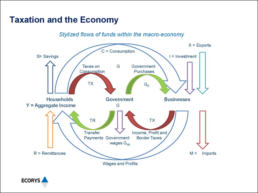
Stylized flow of funds within the macro-economy - 1
• The economic activity of any country can be represented by the
flow of funds within that country’s macro-economy.
• It is convenient to represent the domestic economy as comprising
three sectors: Households, Government and Businesses
(sometimes called the Market sector).
• Imports take funds out the economy and Exports and
Remittances introduce funds into the economy.
• Businesses pay wages to employees and distribute profits to
business owners, either foreigners or in the Household sector.
• Households can spend their current income on Consumption or
add to or subtract from their Savings.
• Businesses require Investment from domestic or foreign sources.

5. Taxation and the Economy

Stylized flows of funds within the macro-economy
X = Exports
C = Consumption
S= Savings
I = Investment
Taxes on
Consumption
G
Government
Purchases
TX
Households
Y = Aggregate Income
GC
Government
Businesses
G
TX
TR
Transfer
Income, Profit and
Payments Government
Border Taxes
wages GW
R = Remittances
M=
Wages and Profits
Imports

6. Taxation and the Economy

Stylized flow of funds within the macro-economy - 3
• In a closed economy, business investment needs, I, must be
funded by Savings (or by Government grants and subsidies).
However, the economy is not closed, and some investment funds
may come from foreign sources.
• The Government is an agent within the economy, purchasing
goods and services, GC, assumed from the business sector, and
paying wages, GW, nominally to the household sector.
• In addition, the government collects taxes, TX, and makes
transfer payments (pensions and social payments) TR to
households.
• The government may also pay subsidies and make grants to the
business sector. These can be included in the definition of TR.

7. Taxation and the Economy

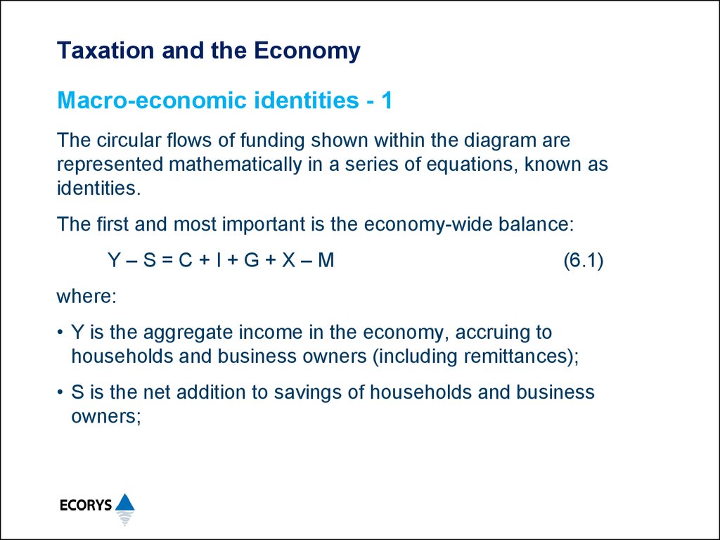
Macro-economic identities - 1
The circular flows of funding shown within the diagram are
represented mathematically in a series of equations, known as
identities.
The first and most important is the economy-wide balance:
Y–S=C+I+G+X–M
(6.1)
where:
• Y is the aggregate income in the economy, accruing to
households and business owners (including remittances);
• S is the net addition to savings of households and business
owners;

8. Taxation and the Economy

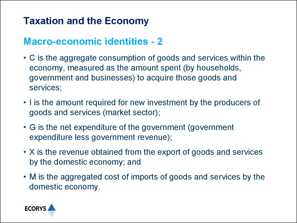
Macro-economic identities - 2
• C is the aggregate consumption of goods and services within the
economy, measured as the amount spent (by households,
government and businesses) to acquire those goods and
services;
• I is the amount required for new investment by the producers of
goods and services (market sector);
• G is the net expenditure of the government (government
expenditure less government revenue);
• X is the revenue obtained from the export of goods and services
by the domestic economy; and
• M is the aggregated cost of imports of goods and services by the
domestic economy.

9. Taxation and the Economy

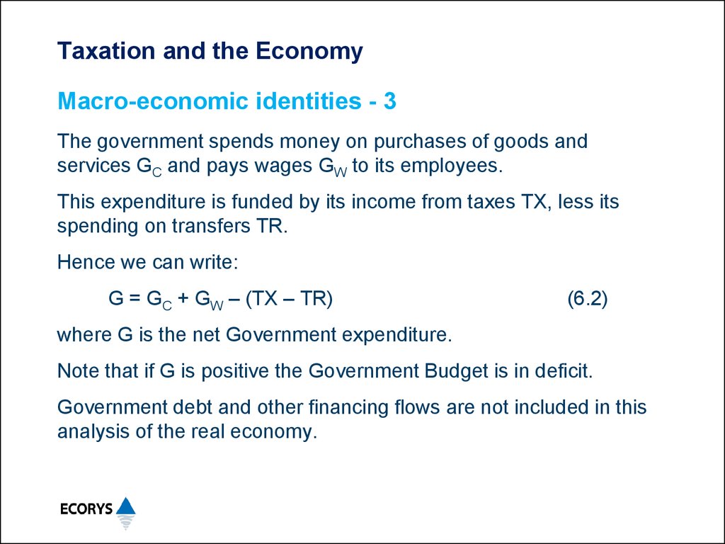
Macro-economic identities - 3
The government spends money on purchases of goods and
services GC and pays wages GW to its employees.
This expenditure is funded by its income from taxes TX, less its
spending on transfers TR.
Hence we can write:
G = GC + GW – (TX – TR)
(6.2)
where G is the net Government expenditure.
Note that if G is positive the Government Budget is in deficit.
Government debt and other financing flows are not included in this
analysis of the real economy.

10. Taxation and the Economy

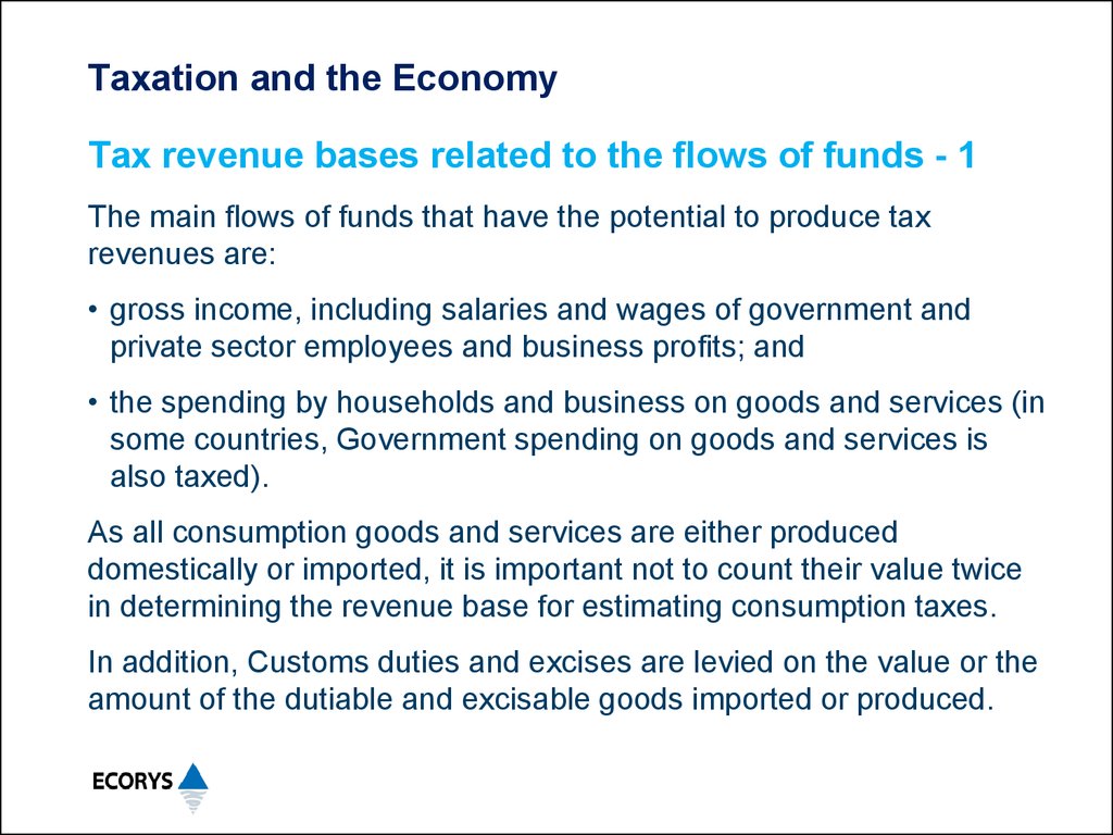
Tax revenue bases related to the flows of funds - 1
The main flows of funds that have the potential to produce tax
revenues are:
• gross income, including salaries and wages of government and
private sector employees and business profits; and
• the spending by households and business on goods and services (in
some countries, Government spending on goods and services is
also taxed).
As all consumption goods and services are either produced
domestically or imported, it is important not to count their value twice
in determining the revenue base for estimating consumption taxes.
In addition, Customs duties and excises are levied on the value or the
amount of the dutiable and excisable goods imported or produced.

11. Taxation and the Economy

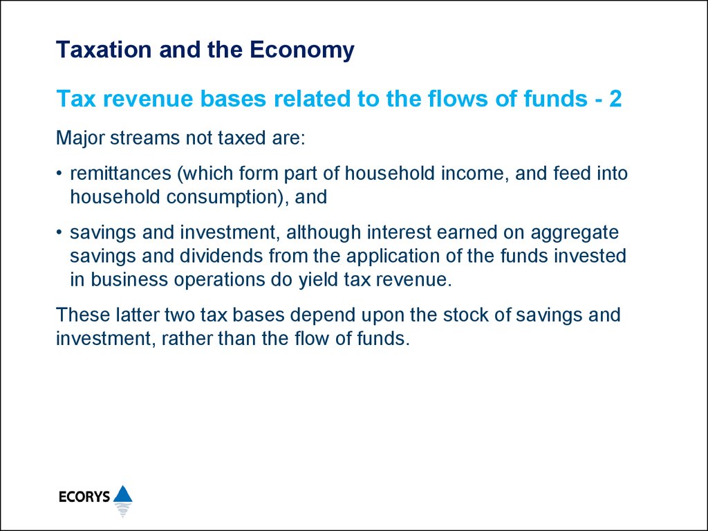
Tax revenue bases related to the flows of funds - 2
Major streams not taxed are:
• remittances (which form part of household income, and feed into
household consumption), and
• savings and investment, although interest earned on aggregate
savings and dividends from the application of the funds invested
in business operations do yield tax revenue.
These latter two tax bases depend upon the stock of savings and
investment, rather than the flow of funds.

12. Taxation and the Economy

Economic bases for forecasting the main taxes - 1
Consumption and other indirect taxes
Value Added Tax
Private final consumption
(household and small businesses)
Excises
Value or quantity of excisable goods
produced or imported
Trade taxes
Import duties and levies
Value of goods imported – ideally by
tariff classification
Export duties and levies
Value of dutiable goods exported ideally by tariff classification

13. Taxation and the Economy

Economic bases for forecasting the main taxes - 2
Income and other direct taxes
Corporate income tax
(profits tax)
Operating surplus of
incorporated entities
Personal income tax
Aggregate salaries, wages, interest
and untaxed profits of entrepreneurs
Payroll tax
Aggregate salaries and wages
Social tax
Aggregate salaries, wages
and entrepreneurial income

14. Revenue Forecasting – Session 2

Tax Elasticity and Tax Buoyancy
• Definitions of tax buoyancy and tax elasticity
• Differences between tax buoyancy and tax elasticity
• Tax buoyancy calculation
• Tax elasticity calculation
• Expected relativity between the measures
• Expected elasticity and buoyancy of specific revenues

15. Tax Elasticity and Tax Buoyancy

Definitions - 1
Tax Buoyancy
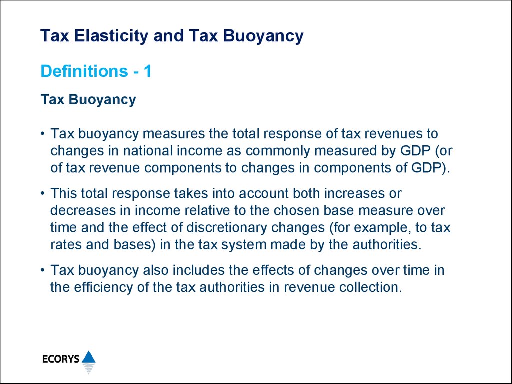
• Tax buoyancy measures the total response of tax revenues to
changes in national income as commonly measured by GDP (or
of tax revenue components to changes in components of GDP).
• This total response takes into account both increases or
decreases in income relative to the chosen base measure over
time and the effect of discretionary changes (for example, to tax
rates and bases) in the tax system made by the authorities.
• Tax buoyancy also includes the effects of changes over time in
the efficiency of the tax authorities in revenue collection.

16. Tax Elasticity and Tax Buoyancy

Definitions - 2
Tax Elasticity
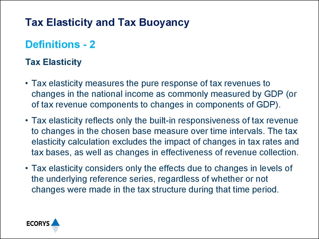
• Tax elasticity measures the pure response of tax revenues to
changes in the national income as commonly measured by GDP (or
of tax revenue components to changes in components of GDP).
• Tax elasticity reflects only the built-in responsiveness of tax revenue
to changes in the chosen base measure over time intervals. The tax
elasticity calculation excludes the impact of changes in tax rates and
tax bases, as well as changes in effectiveness of revenue collection.
• Tax elasticity considers only the effects due to changes in levels of
the underlying reference series, regardless of whether or not
changes were made in the tax structure during that time period.

17. Tax Elasticity and Tax Buoyancy

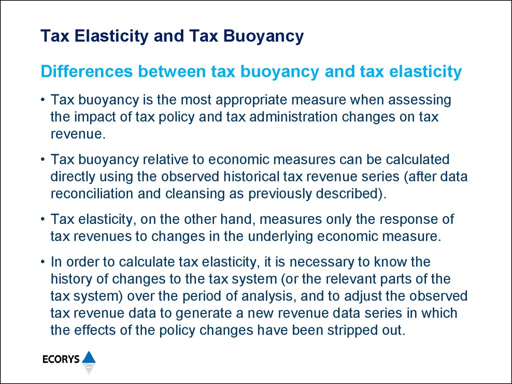
Differences between tax buoyancy and tax elasticity
• Tax buoyancy is the most appropriate measure when assessing
the impact of tax policy and tax administration changes on tax
revenue.
• Tax buoyancy relative to economic measures can be calculated
directly using the observed historical tax revenue series (after data
reconciliation and cleansing as previously described).
• Tax elasticity, on the other hand, measures only the response of
tax revenues to changes in the underlying economic measure.
• In order to calculate tax elasticity, it is necessary to know the
history of changes to the tax system (or the relevant parts of the
tax system) over the period of analysis, and to adjust the observed
tax revenue data to generate a new revenue data series in which
the effects of the policy changes have been stripped out.

18. Tax Elasticity and Tax Buoyancy

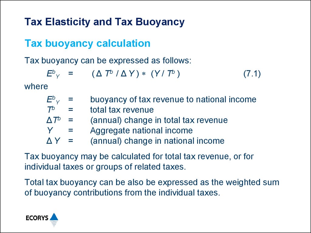
Tax buoyancy calculation
Tax buoyancy can be expressed as follows:
EbY =
( Δ Tb / Δ Y ) (Y / Tb )
(7.1)
where
EbY =
buoyancy of tax revenue to national income
Tb
=
total tax revenue
ΔTb =
(annual) change in total tax revenue
Y
=
Aggregate national income
ΔY =
(annual) change in national income
Tax buoyancy may be calculated for total tax revenue, or for
individual taxes or groups of related taxes.
Total tax buoyancy can be also be expressed as the weighted sum
of buoyancy contributions from the individual taxes.

19. Tax Elasticity and Tax Buoyancy

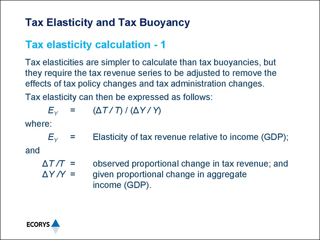
Tax elasticity calculation - 1
Tax elasticities are simpler to calculate than tax buoyancies, but
they require the tax revenue series to be adjusted to remove the
effects of tax policy changes and tax administration changes.
Tax elasticity can then be expressed as follows:
EY =
(ΔT / T) / (ΔY / Y)
where:
EY =
Elasticity of tax revenue relative to income (GDP);
and
ΔT /T =
observed proportional change in tax revenue; and
ΔY /Y =
given proportional change in aggregate
income (GDP).

20. Tax Elasticity and Tax Buoyancy

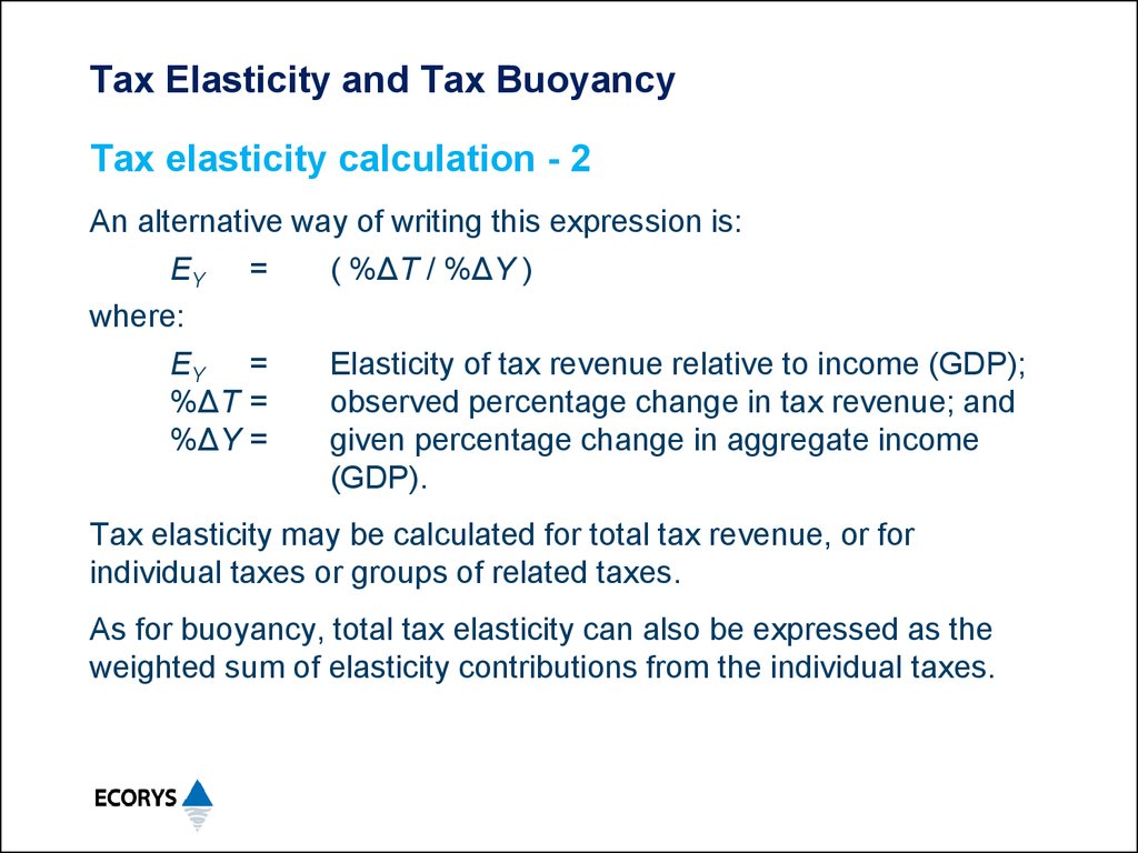
Tax elasticity calculation - 2
An alternative way of writing this expression is:
EY =
( %ΔT / %ΔY )
where:
EY =
Elasticity of tax revenue relative to income (GDP);
%ΔT =
observed percentage change in tax revenue; and
%ΔY =
given percentage change in aggregate income
(GDP).
Tax elasticity may be calculated for total tax revenue, or for
individual taxes or groups of related taxes.
As for buoyancy, total tax elasticity can also be expressed as the
weighted sum of elasticity contributions from the individual taxes.

21. Tax Elasticity and Tax Buoyancy

Expected relativity between the measures - 1
• Each of the measures, Buoyancy and Elasticity, may have values
less than unity, equal to unity, or greater than unity, when
different taxes are compared to relevant economic variables (or
other specific tax bases).
• Where there have been no policy changes, then tax buoyancy is
expected to be equal to tax elasticity.

22. Tax Elasticity and Tax Buoyancy

Expected relativity between the measures - 2
• When tax policy changes have increased effective tax rates, such
as an increase in the rate of corporate profit tax, then the
buoyancy of that tax will be greater than its elasticity, when both
are measured relative to the same economic series (operating
surplus of corporates) or other revenue base (corporate profits).
• When tax policy changes have decreased effective tax rates,
such as an increase in capital allowances (through increased
depreciation rates or allowing the immediate deduction of a class
of assets), then the buoyancy will be less than the elasticity,
when both are measured relative to the same revenue base.

23. Tax Elasticity and Tax Buoyancy

Elasticity and buoyancy for specific revenues - 1
Firstly, in terms of elasticity of taxes relative to GDP or its
relevant main components, the general expectation is as follows:
• Personal Income Taxes (PIT) tend to have E > 1, owing to the
progressive tax rate structure (tax rates increasing with income),
with values of E up to1.35 being observed in some western
economies during periods of higher annual wage growth, and
values nearer to.1.20 when wages are growing more slowly.
• For corporate income or profit taxes, the value of E may be above
or below unity, depending upon the economic or revenue base
chosen, and the dynamics of the business investment cycle.

24. Tax Elasticity and Tax Buoyancy

Elasticity and buoyancy for specific revenues - 2
• In periods of higher investment, the capital allowances reduce
taxable income growth relative to the growth of most economic
base series, so the value of E tends to fall.
• In economic downturns, when investment spending is often cut
back, the value of E measured relative to broad based profit
series (operating surplus) is likely to rise.
• However, if the rate of growth in corporate profits falls relative to
that of GDP, the value of E measured against GDP may fall at the
same time.
• Corporate incomes and profit taxes are among the most difficult
series to forecast, even during periods of relatively steady
economic growth.

25. Tax Elasticity and Tax Buoyancy

Elasticity and buoyancy for specific revenues - 3
• Value Added Taxes (VAT) tend to have E ~ 1.0, relative to GDP
as a whole and relative to domestic private final consumption,
provided that excess VAT paid by registered payers is refundable
within a realistic period, and the VAT is applied to imports and
exported goods qualify for VAT refunds.
• If basic goods (such as food) are exempted from VAT, then the
value of E for VAT is expected to be slightly greater than 1.0,
measured against consumption or against GDP.

26. Tax Elasticity and Tax Buoyancy

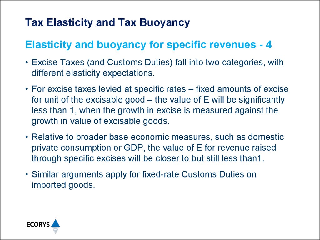
Elasticity and buoyancy for specific revenues - 4
• Excise Taxes (and Customs Duties) fall into two categories, with
different elasticity expectations.
• For excise taxes levied at specific rates – fixed amounts of excise
for unit of the excisable good – the value of E will be significantly
less than 1, when the growth in excise is measured against the
growth in value of excisable goods.
• Relative to broader base economic measures, such as domestic
private consumption or GDP, the value of E for revenue raised
through specific excises will be closer to but still less than1.
• Similar arguments apply for fixed-rate Customs Duties on
imported goods.

27. Tax Elasticity and Tax Buoyancy

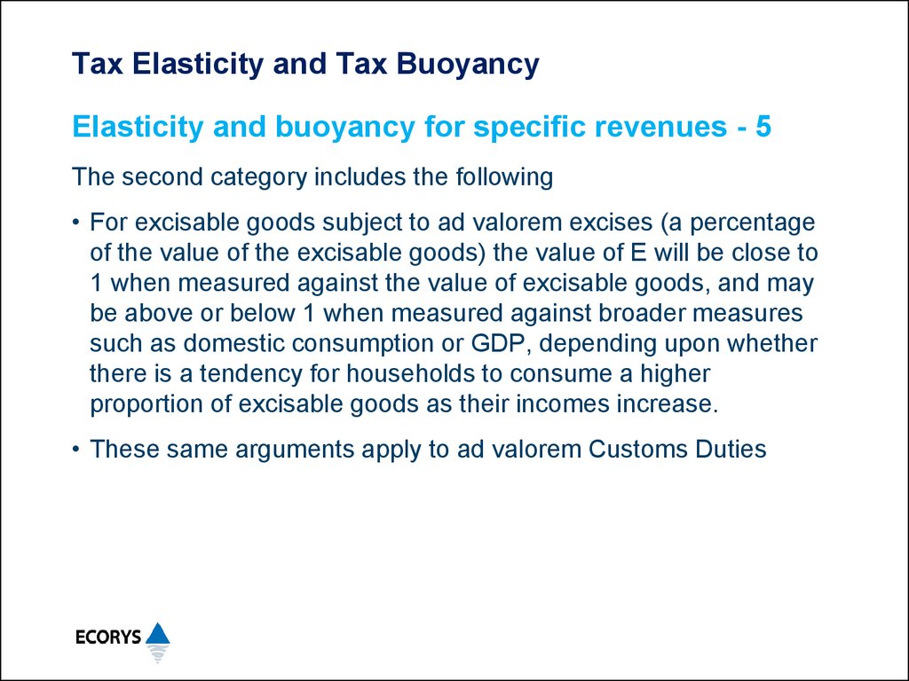
Elasticity and buoyancy for specific revenues - 5
The second category includes the following
• For excisable goods subject to ad valorem excises (a percentage
of the value of the excisable goods) the value of E will be close to
1 when measured against the value of excisable goods, and may
be above or below 1 when measured against broader measures
such as domestic consumption or GDP, depending upon whether
there is a tendency for households to consume a higher
proportion of excisable goods as their incomes increase.
• These same arguments apply to ad valorem Customs Duties

28. Tax Elasticity and Tax Buoyancy

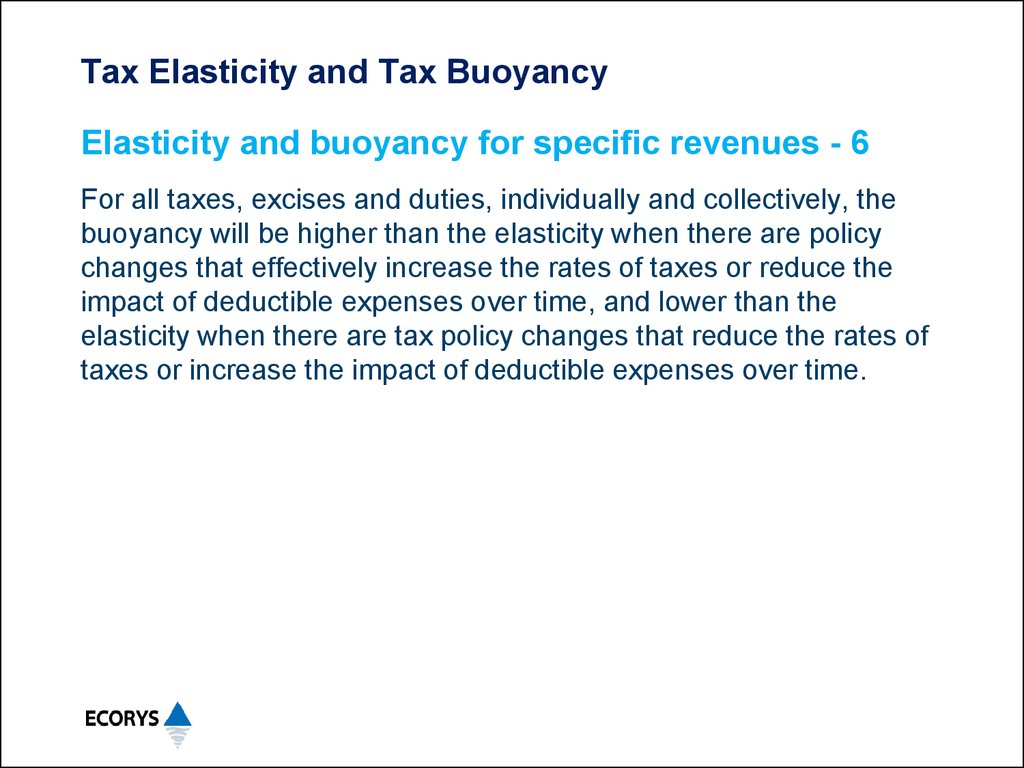
Elasticity and buoyancy for specific revenues - 6
For all taxes, excises and duties, individually and collectively, the
buoyancy will be higher than the elasticity when there are policy
changes that effectively increase the rates of taxes or reduce the
impact of deductible expenses over time, and lower than the
elasticity when there are tax policy changes that reduce the rates of
taxes or increase the impact of deductible expenses over time.

29. Revenue Forecasting – Session 3

Revenue Forecasting using Macroeconomic Data
• General approach to forecasting revenues using
forecasts of macroeconomic variables
• Example of estimation of total revenue and total tax
revenue buoyancies relative to GDP
• Practical exercises

30. Revenue Forecasting using Macroeconomic Data

Forecasting revenues using forecasts of
macroeconomic variables - 1
• This methodology requires the use of a consistent set of macroeconomic forecasts covering the period over which revenues are
to be forecast. It also requires at least three years of historical
data for the macro-economic variables as well as for the
revenues to be forecasted.
• The latter are required to determine the relationship between the
rate of growth of the revenues to be forecasted and the rate of
growth of the corresponding macro-economic variables.
• In other words, sufficient historical data is required to be able to
calculate the buoyancies of the revenue series to be forecast,
relative to the macro-economic data series.

31. Revenue Forecasting using Macroeconomic Data

Forecasting revenues using forecasts of
macroeconomic variables - 2
The data treatment and calculation steps include:
a.
Review and adjust revenue series for the impact of historical
revenue policy changes.
b.
Review and adjust revenue and economic series for the
impact of historical changes in economic policy.
c.
Review historical inflation and price changes and construct
deflated real historical data for revenues and macroeconomic
series of interest (this step may sometimes be omitted)
d.
Determine revenue elasticities from the growth in adjusted
and deflated revenues compare to adjusted and deflated
GDP (or components of GDP)
• e.

32. Revenue Forecasting using Macroeconomic Data

Forecasting revenues using forecasts of
macroeconomic variables - 3
The remaining data treatment and calculation steps include:
e.
Use these elasticities to forecast real revenues using
forecasts of real macroeconomic variables.
f.
Convert forecasts into nominal values using expected
inflation factors for revenues and macroeconomic data series.
g.
Adjust forecasts of revenues for anticipated changes in
revenue policies and in economic policies that are expected
to affect revenues.
h. Adopt the completed revenue forecasts.
Nominal values can be used if the deflators for the tax and economic
variables are identical (or one is seen as the best proxy for the other).

33. Revenue Forecasting using Macroeconomic Data

Example of estimation of total revenue buoyancy
and total tax revenue buoyancy relative to GDP - 1
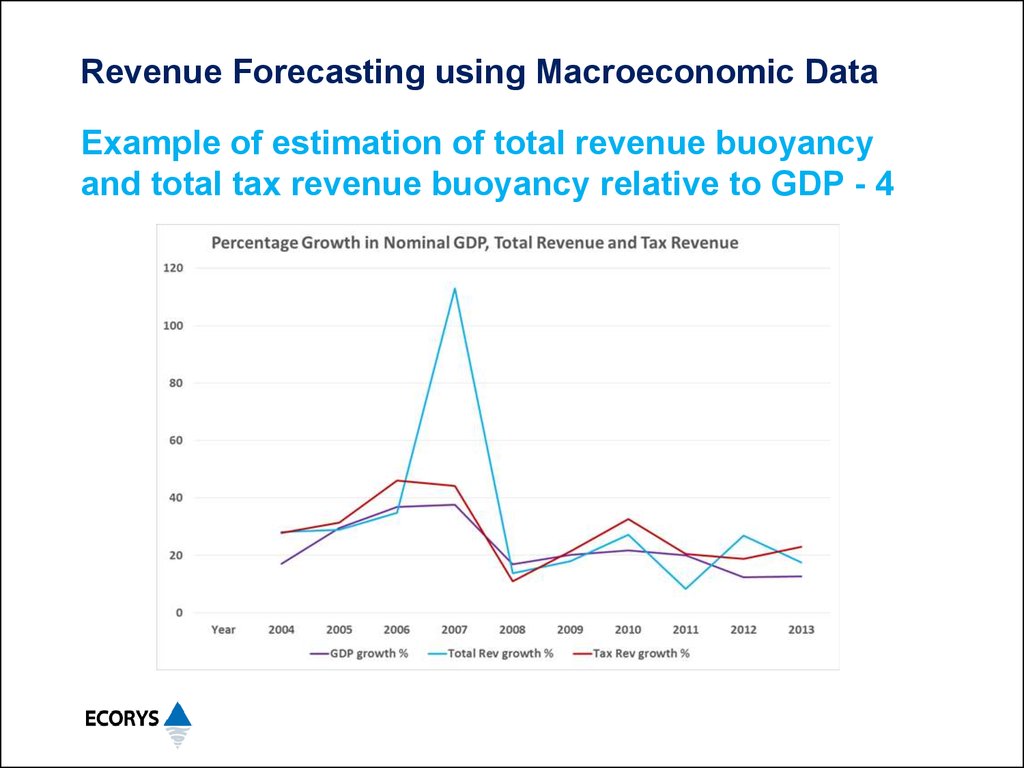
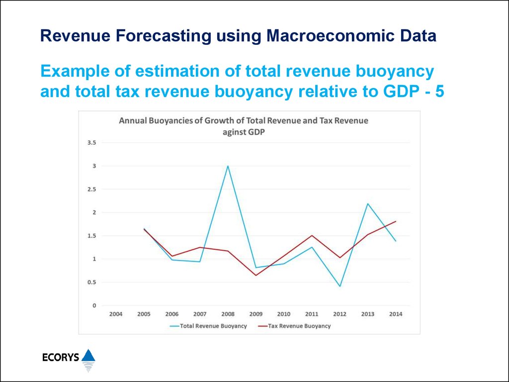
• Using data from the Implementation of the State Budget, 20002014, it is possible to calculate the buoyancies for Total revenue
and for Total Tax Revenue measured against GDP.
• The results of this exercise are shown graphically in a series of
slides and a copy of the worksheet is available on your computer.

34. Revenue Forecasting using Macroeconomic Data

Example of estimation of total revenue buoyancy
and total tax revenue buoyancy relative to GDP - 2

35. Revenue Forecasting using Macroeconomic Data

Example of estimation of total revenue buoyancy
and total tax revenue buoyancy relative to GDP - 3

36. Revenue Forecasting using Macroeconomic Data

Example of estimation of total revenue buoyancy
and total tax revenue buoyancy relative to GDP - 4

37. Revenue Forecasting using Macroeconomic Data

Example of estimation of total revenue buoyancy
and total tax revenue buoyancy relative to GDP - 5

38. Revenue Forecasting using Macroeconomic Data

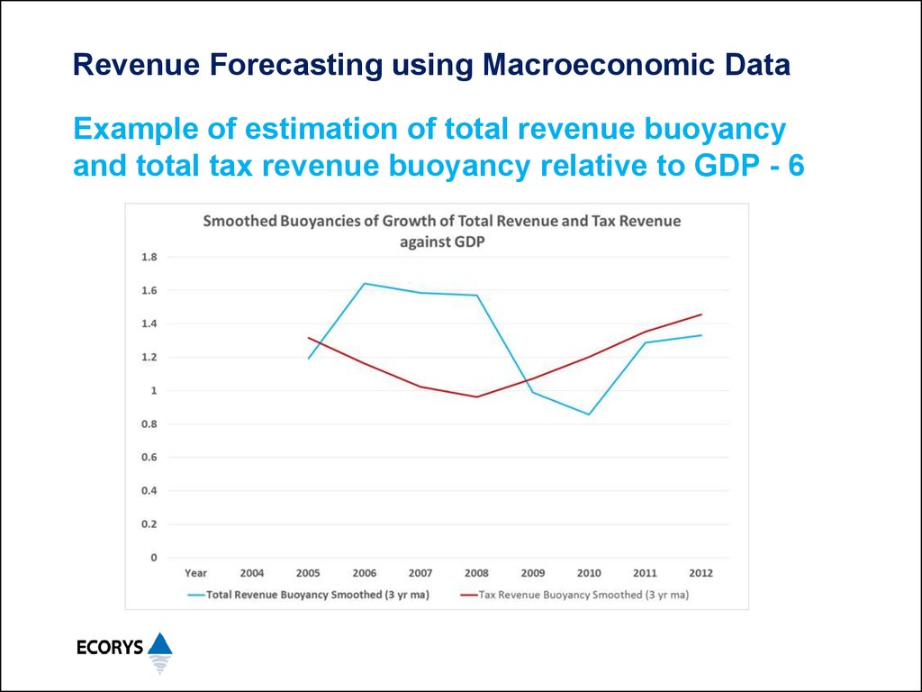
Example of estimation of total revenue buoyancy
and total tax revenue buoyancy relative to GDP - 6

39. Revenue Forecasting using Macroeconomic Data

Example of estimation of total revenue buoyancy
and total tax revenue buoyancy relative to GDP - 7
• Because there is no policy related information available about the
historical revenues, we can calculate only revenue buoyancies
for use in forecasting future total revenue and tax revenue.
• Owing to the somewhat erratic variations in buoyancies from year
to year, for both total revenue and tax revenue, even in the most
recent three years (2011-2014), the data have been smoothed
through averaging over successive three year periods in the final
chart.
• Fortunately, the smoothed buoyancies for both total revenue and
tax revenue relative to GDP show much more stability over the
last two years of the evaluation period. The values chosen are
averages of the smoothed values for each of these two years.

40. Revenue Forecasting using Macroeconomic Data

Example of estimation of total revenue buoyancy
and total tax revenue buoyancy relative to GDP - 8
• The calculated results are Eb (total revenue to GDP) = 1.31 and
Eb (tax revenue to GDP) = 1.40. Both of these figures are
significantly greater than unity, implying strong growth in
revenues relative to GDP.
• The revenue system of Tajikistan has been relatively buoyant
over this period, more so than in many other countries.
• Note that the averages over the entire period for the unsmoothed
buoyancies are 1.35 for total revenue and 1.27 for tax revenue.
But given the extreme variations in the earlier part of the series,
these averages are unreliable for forecasting forward from 2014.

41. Revenue Forecasting using Macroeconomic Data

Example of estimation of total revenue buoyancy
and total tax revenue buoyancy relative to GDP - 9
• In summary, we expect total revenue in 2015 (and subsequently)
to grow by 1.31 times the rate of growth of nominal GDP, and tax
revenue in 2015 and in later years) to grow by 1.40 times the rate
of growth of nominal GDP.
• Given forecasts of nominal GDP, both total revenue and tax
revenue can also be forecast for several years ahead.
• Ideally, the causes of the erratic growth in revenues in the early
part of the period should be determined. Further, the revenue
impact of all policy and administrative changes over the historical
period should be determined, and adjusted tax and total revenue
series used to calculate revenue elasticities for use in forecasts.

42. Revenue Forecasting using Macroeconomic Data

Practical examples
Examples of actual revenue forecasts using this methodology
require the current forecasts of macroeconomic variables.
If these are made available within the next few days, we will be
able to test this forecasting approach using data for Tajikistan.
Alternatively, we can develop and compare forecasts using data
from other countries.