 software
Similar presentations:


")


")


Seismic image regression
1.
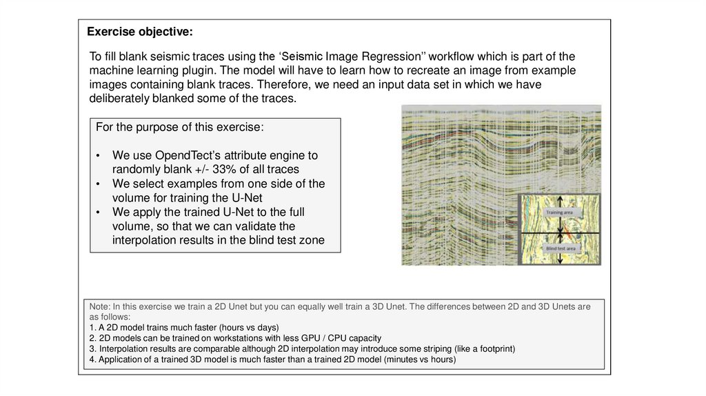
Exercise objective:To fill blank seismic traces using the ‘Seismic Image Regression’’ workflow which is part of the
machine learning plugin. The model will have to learn how to recreate an image from example
images containing blank traces. Therefore, we need an input data set in which we have
deliberately blanked some of the traces.
For the purpose of this exercise:
We use OpendTect’s attribute engine to
randomly blank +/- 33% of all traces
We select examples from one side of the
volume for training the U-Net
We apply the trained U-Net to the full
volume, so that we can validate the
interpolation results in the blind test zone
Note: In this exercise we train a 2D Unet but you can equally well train a 3D Unet. The differences between 2D and 3D Unets are
as follows:
1. A 2D model trains much faster (hours vs days)
2. 2D models can be trained on workstations with less GPU / CPU capacity
3. Interpolation results are comparable although 2D interpolation may introduce some striping (like a footprint)
4. Application of a trained 3D model is much faster than a trained 2D model (minutes vs hours)
2.
Randomly blank traces workflow:To train our 2D Unet regression model we create a data set with 33% randomly blanked traces.
From this cube we extract examples for training in a restricted area. The trained model is
applied to the entire volume, whereby the area from which no examples are extracted acts as
blind test area. The real value is of course when we apply the trained model to an area with
real missing traces (which we don’t have in this case). Random blanking (replacing the values
with hard zeros) is done in OpendTect’s Attribute engine and can be done in different ways. In
this case, we will create an attribute set to perform the following tasks:
1. Math attribute with formula: “randg(1)”. This generates random values with a Gaussian
distribution and 1 standard deviation;
2. Apply this attribute to a horizon and save as horizon data;
3. Horizon attribute that retrieves the random values from the saved horizon data. A Horizon
attribute replaces a value at an inline, crossline position with the value extracted from the
given horizon;
4. Math attribute with formula: “abs(value)> 1 ? 0: seis”. We assign the retrieved horizon data
to the variable “value” and the seismic data to “seis”. This attribute assigns values larger
than the absolute value of 1 standard deviation to zero while all other values are given the
value of the seismic data.
5. Additional attributes in the set are used to compare/QC results before and after prediction.
3.
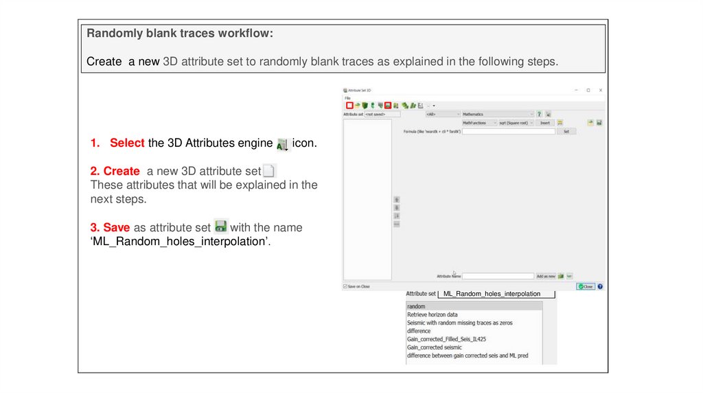
Randomly blank traces workflow:Create a new 3D attribute set to randomly blank traces as explained in the following steps.
1. Select the 3D Attributes engine
icon.
2. Create a new 3D attribute set
These attributes that will be explained in the
next steps.
3. Save as attribute set
with the name
‘ML_Random_holes_interpolation’.
ML_Random_holes_interpolation
4.
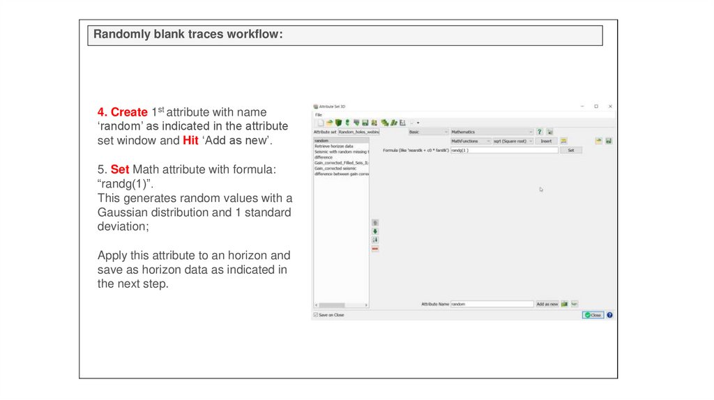
Randomly blank traces workflow:4. Create 1st attribute with name
‘random’ as indicated in the attribute
set window and Hit ‘Add as new’.
5. Set Math attribute with formula:
“randg(1)”.
This generates random values with a
Gaussian distribution and 1 standard
deviation;
Apply this attribute to an horizon and
save as horizon data as indicated in
the next step.
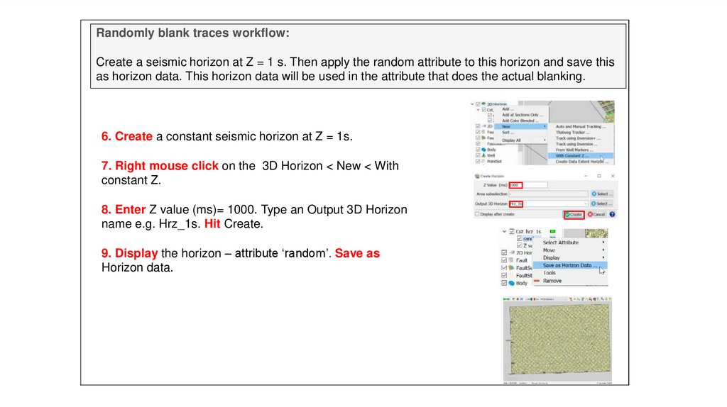
5.
Randomly blank traces workflow:Create a seismic horizon at Z = 1 s. Then apply the random attribute to this horizon and save this
as horizon data. This horizon data will be used in the attribute that does the actual blanking.
6. Create a constant seismic horizon at Z = 1s.
7. Right mouse click on the 3D Horizon < New < With
constant Z.
8. Enter Z value (ms)= 1000. Type an Output 3D Horizon
name e.g. Hrz_1s. Hit Create.
9. Display the horizon – attribute ‘random’. Save as
Horizon data.
6.
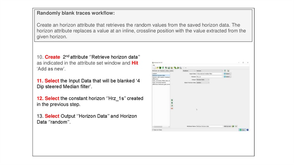
Randomly blank traces workflow:Create an horizon attribute that retrieves the random values from the saved horizon data. The
horizon attribute replaces a value at an inline, crossline position with the value extracted from the
given horizon.
10. Create 2nd attribute ‘’Retrieve horizon data’’
as indicated in the attribute set window and Hit
‘Add as new’.
11. Select the Input Data that will be blanked ‘4
Dip steered Median filter’.
12. Select the constant horizon ‘’Hrz_1s’’ created
in the previous step.
13. Select Output ‘’Horizon Data’’ and Horizon
Data ‘’random’’.
7.
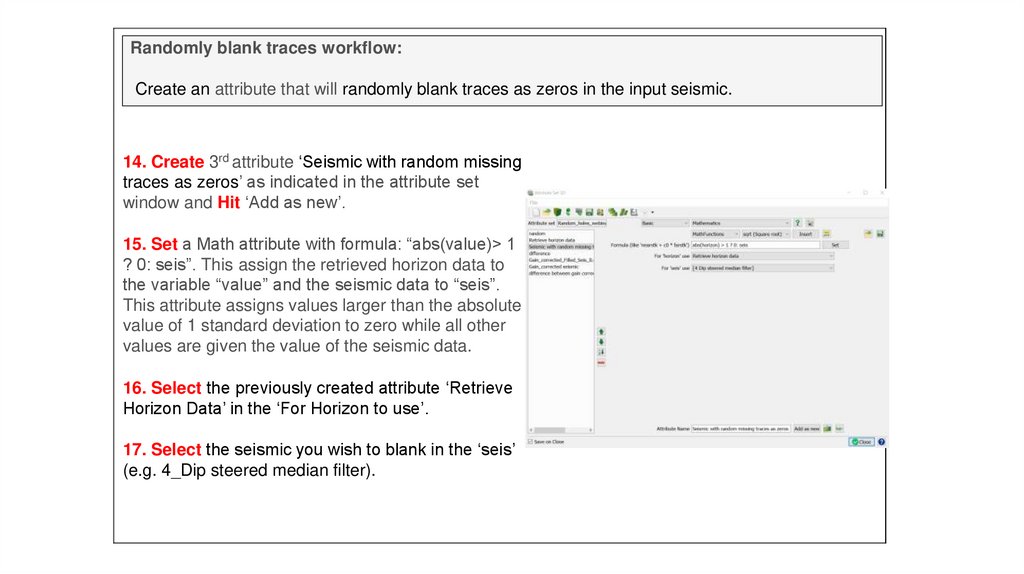
Randomly blank traces workflow:Create an attribute that will randomly blank traces as zeros in the input seismic.
14. Create 3rd attribute ‘Seismic with random missing
traces as zeros’ as indicated in the attribute set
window and Hit ‘Add as new’.
15. Set a Math attribute with formula: “abs(value)> 1
? 0: seis”. This assign the retrieved horizon data to
the variable “value” and the seismic data to “seis”.
This attribute assigns values larger than the absolute
value of 1 standard deviation to zero while all other
values are given the value of the seismic data.
16. Select the previously created attribute ‘Retrieve
Horizon Data’ in the ‘For Horizon to use’.
17. Select the seismic you wish to blank in the ‘seis’
(e.g. 4_Dip steered median filter).
8.
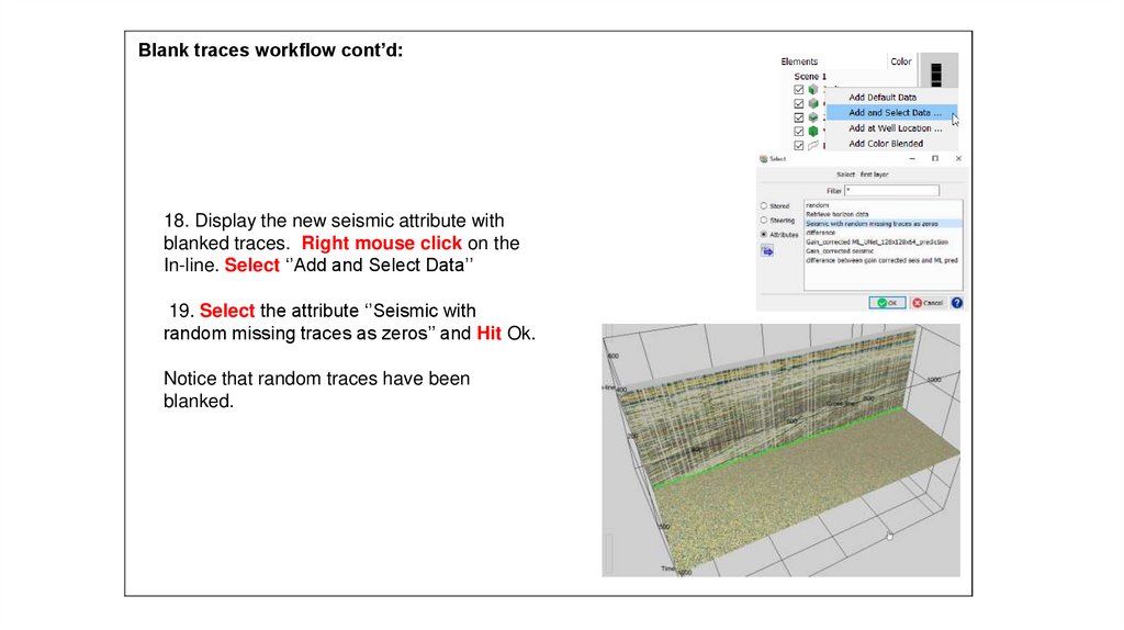
Blank traces workflow cont’d:18. Display the new seismic attribute with
blanked traces. Right mouse click on the
In-line. Select ‘’Add and Select Data’’
19. Select the attribute ‘’Seismic with
random missing traces as zeros’’ and Hit Ok.
Notice that random traces have been
blanked.
9.
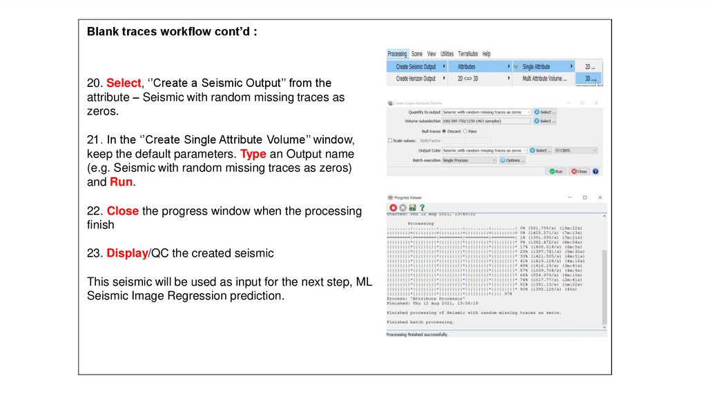
Blank traces workflow cont’d :20. Select, ‘’Create a Seismic Output’’ from the
attribute – Seismic with random missing traces as
zeros.
21. In the ‘’Create Single Attribute Volume’’ window,
keep the default parameters. Type an Output name
(e.g. Seismic with random missing traces as zeros)
and Run.
22. Close the progress window when the processing
finish
23. Display/QC the created seismic
This seismic will be used as input for the next step, ML
Seismic Image Regression prediction.
10.
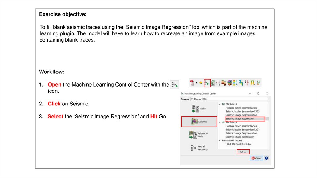
Exercise objective:To fill blank seismic traces using the ‘Seismic Image Regression’’ tool which is part of the machine
learning plugin. The model will have to learn how to recreate an image from example images
containing blank traces.
Workflow:
1. Open the Machine Learning Control Center with the
icon.
2. Click on Seismic.
3. Select the ‘Seismic Image Regression’ and Hit Go.
11.
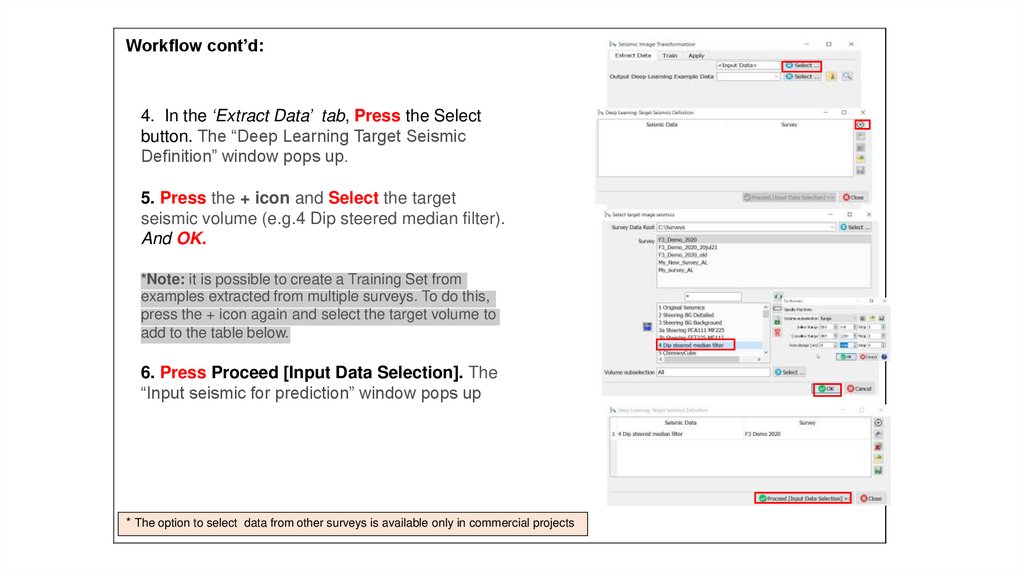
Workflow cont’d:4. In the ‘Extract Data’ tab, Press the Select
button. The “Deep Learning Target Seismic
Definition” window pops up.
5. Press the + icon and Select the target
seismic volume (e.g.4 Dip steered median filter).
And OK.
*Note: it is possible to create a Training Set from
examples extracted from multiple surveys. To do this,
press the + icon again and select the target volume to
add to the table below.
6. Press Proceed [Input Data Selection]. The
“Input seismic for prediction” window pops up
* The option to select data from other surveys is available only in commercial projects
12.
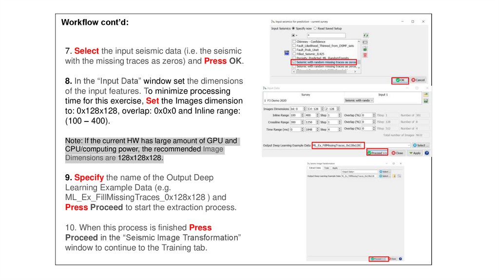
Workflow cont’d:7. Select the input seismic data (i.e. the seismic
with the missing traces as zeros) and Press OK.
8. In the “Input Data” window set the dimensions
of the input features. To minimize processing
time for this exercise, Set the Images dimension
to: 0x128x128, overlap: 0x0x0 and Inline range:
(100 – 400).
Note: If the current HW has large amount of GPU and
CPU/computing power, the recommended Image
Dimensions are 128x128x128.
9. Specify the name of the Output Deep
Learning Example Data (e.g.
ML_Ex_FillMissingTraces_0x128x128 ) and
Press Proceed to start the extraction process.
10. When this process is finished Press
Proceed in the “Seismic Image Transformation”
window to continue to the Training tab.
13.
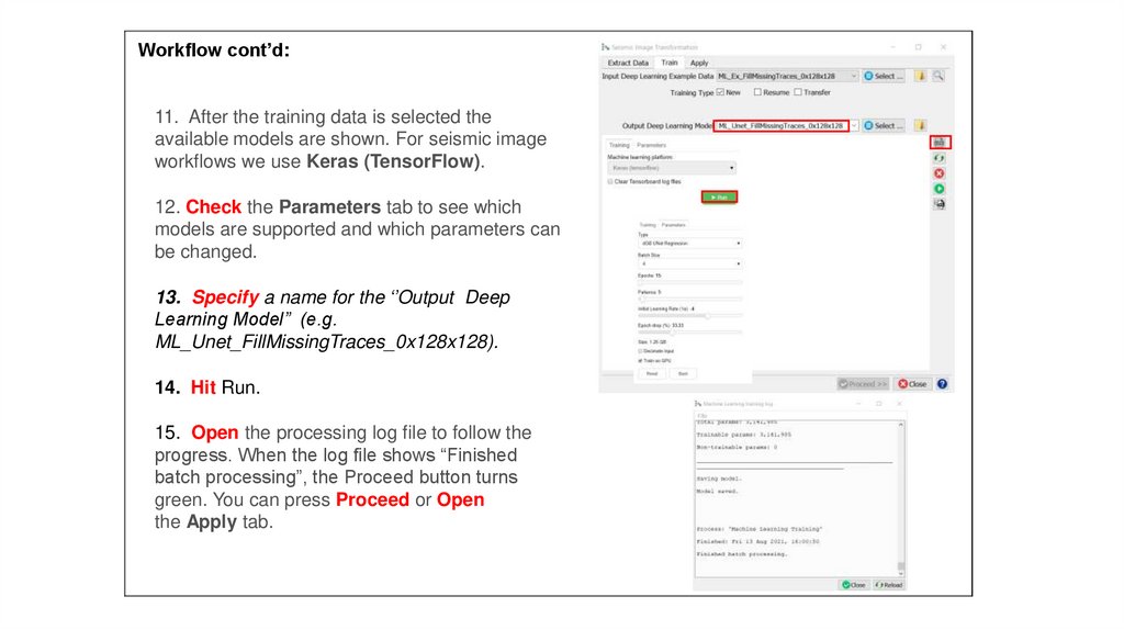
Workflow cont’d:11. After the training data is selected the
available models are shown. For seismic image
workflows we use Keras (TensorFlow).
12. Check the Parameters tab to see which
models are supported and which parameters can
be changed.
13. Specify a name for the ‘’Output Deep
Learning Model’’ (e.g.
ML_Unet_FillMissingTraces_0x128x128).
14. Hit Run.
15. Open the processing log file to follow the
progress. When the log file shows “Finished
batch processing”, the Proceed button turns
green. You can press Proceed or Open
the Apply tab.
14.
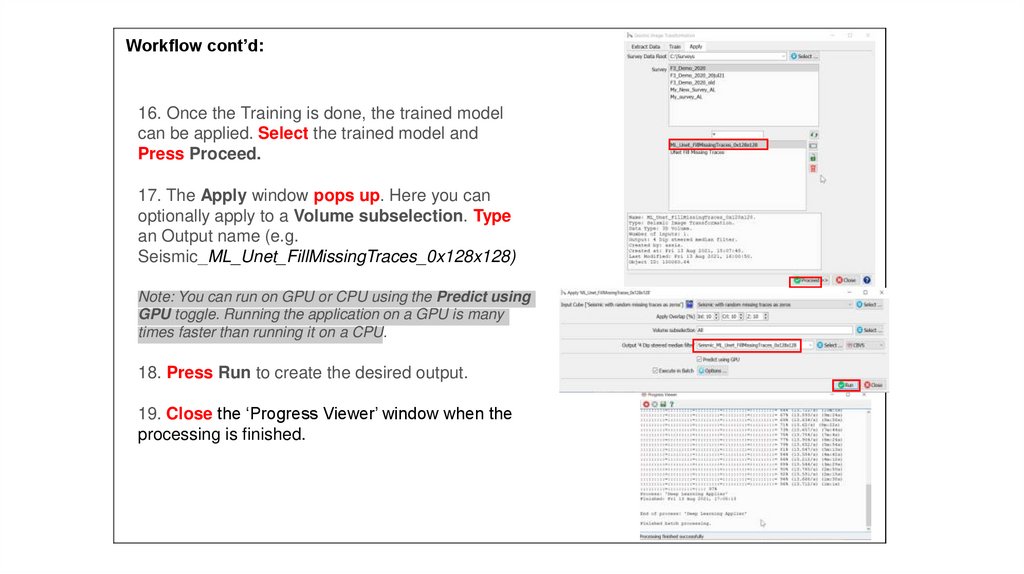
Workflow cont’d:16. Once the Training is done, the trained model
can be applied. Select the trained model and
Press Proceed.
17. The Apply window pops up. Here you can
optionally apply to a Volume subselection. Type
an Output name (e.g.
Seismic_ML_Unet_FillMissingTraces_0x128x128)
Note: You can run on GPU or CPU using the Predict using
GPU toggle. Running the application on a GPU is many
times faster than running it on a CPU.
18. Press Run to create the desired output.
19. Close the ‘Progress Viewer’ window when the
processing is finished.
15.
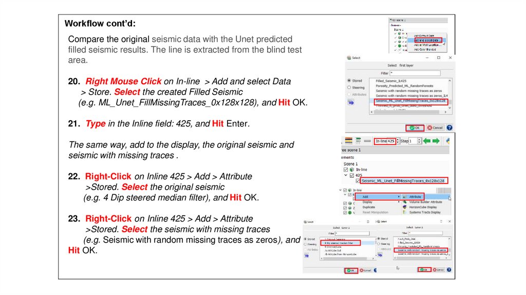
Workflow cont’d:Compare the original seismic data with the Unet predicted
filled seismic results. The line is extracted from the blind test
area.
20. Right Mouse Click on In-line > Add and select Data
> Store. Select the created Filled Seismic
(e.g. ML_Unet_FillMissingTraces_0x128x128), and Hit OK.
21. Type in the Inline field: 425, and Hit Enter.
The same way, add to the display, the original seismic and
seismic with missing traces .
22. Right-Click on Inline 425 > Add > Attribute
>Stored. Select the original seismic
(e.g. 4 Dip steered median filter), and Hit OK.
23. Right-Click on Inline 425 > Add > Attribute
>Stored. Select the seismic with missing traces
(e.g. Seismic with random missing traces as zeros), and
Hit OK.
16.
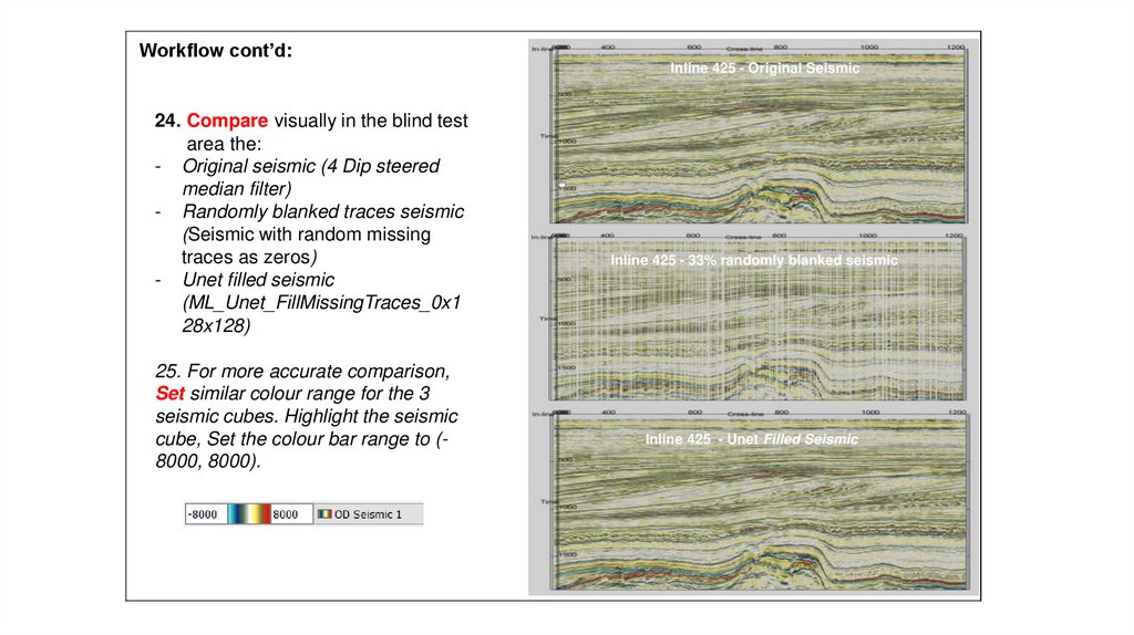
Workflow cont’d:Inline 425 - Original Seismic
24. Compare visually in the blind test
area the:
- Original seismic (4 Dip steered
median filter)
- Randomly blanked traces seismic
(Seismic with random missing
traces as zeros)
- Unet filled seismic
(ML_Unet_FillMissingTraces_0x1
28x128)
25. For more accurate comparison,
Set similar colour range for the 3
seismic cubes. Highlight the seismic
cube, Set the colour bar range to (8000, 8000).
Inline 425 - 33% randomly blanked seismic
Inline 425 - Unet Filled Seismic
17.
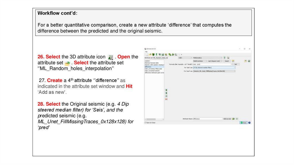
Workflow cont’d:For a better quantitative comparison, create a new attribute ‘difference’ that computes the
difference between the predicted and the original seismic.
26. Select the 3D attribute icon
. Open the
attribute set
. Select the attribute set
‘’ML_Random_holes_interpolation’’
27. Create a 4th attribute ‘’difference’’ as
indicated in the attribute set window and Hit
‘Add as new’.
28. Select the Original seismic (e.g. 4 Dip
steered median filter) for ‘Seis’, and the
predicted seismic (e.g.
ML_Unet_FillMissingTraces_0x128x128) for
‘pred’
18.
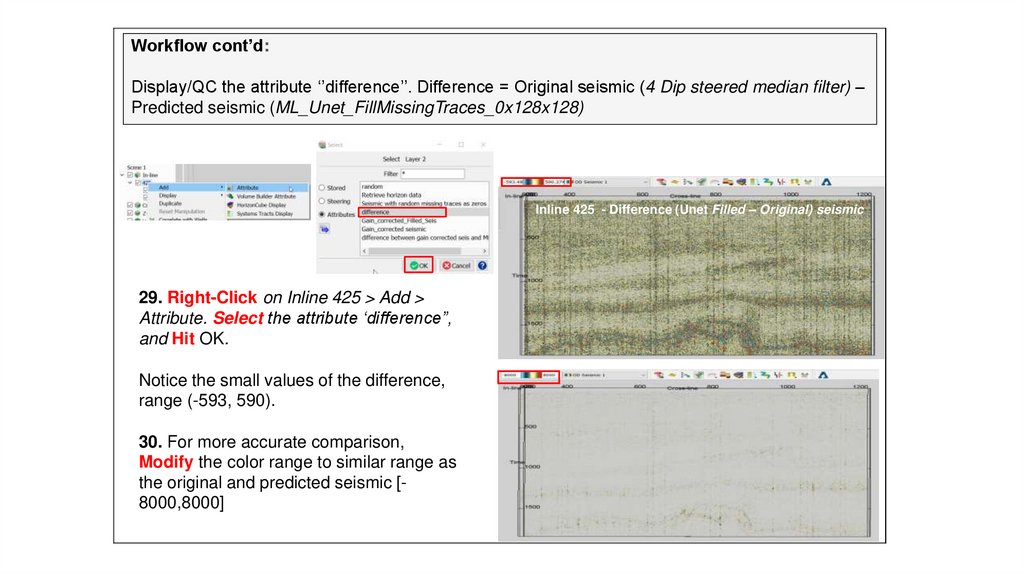
Workflow cont’d:Display/QC the attribute ‘’difference’’. Difference = Original seismic (4 Dip steered median filter) –
Predicted seismic (ML_Unet_FillMissingTraces_0x128x128)
Inline 425 - Difference (Unet Filled – Original) seismic
29. Right-Click on Inline 425 > Add >
Attribute. Select the attribute ‘difference’’,
and Hit OK.
Notice the small values of the difference,
range (-593, 590).
30. For more accurate comparison,
Modify the color range to similar range as
the original and predicted seismic [8000,8000]
19.
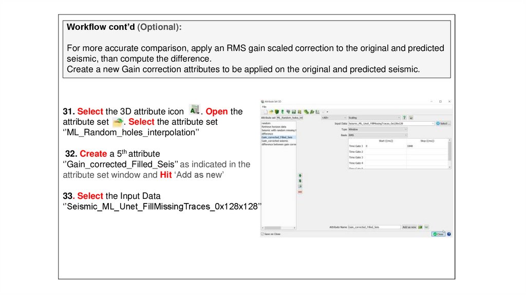
Workflow cont’d (Optional):For more accurate comparison, apply an RMS gain scaled correction to the original and predicted
seismic, than compute the difference.
Create a new Gain correction attributes to be applied on the original and predicted seismic.
31. Select the 3D attribute icon
. Open the
attribute set
. Select the attribute set
‘’ML_Random_holes_interpolation’’
32. Create a 5th attribute
‘’Gain_corrected_Filled_Seis’’ as indicated in the
attribute set window and Hit ‘Add as new’
33. Select the Input Data
‘’Seismic_ML_Unet_FillMissingTraces_0x128x128’’
20.
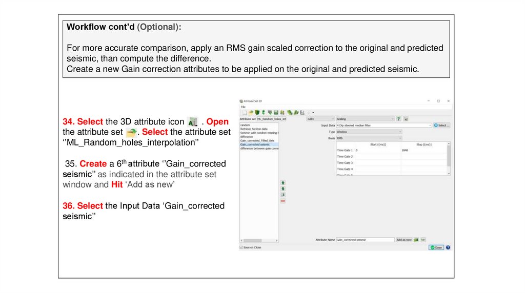
Workflow cont’d (Optional):For more accurate comparison, apply an RMS gain scaled correction to the original and predicted
seismic, than compute the difference.
Create a new Gain correction attributes to be applied on the original and predicted seismic.
34. Select the 3D attribute icon
. Open
the attribute set
. Select the attribute set
‘’ML_Random_holes_interpolation’’
35. Create a 6th attribute ‘’Gain_corrected
seismic’’ as indicated in the attribute set
window and Hit ‘Add as new’
36. Select the Input Data ‘Gain_corrected
seismic’’
21.
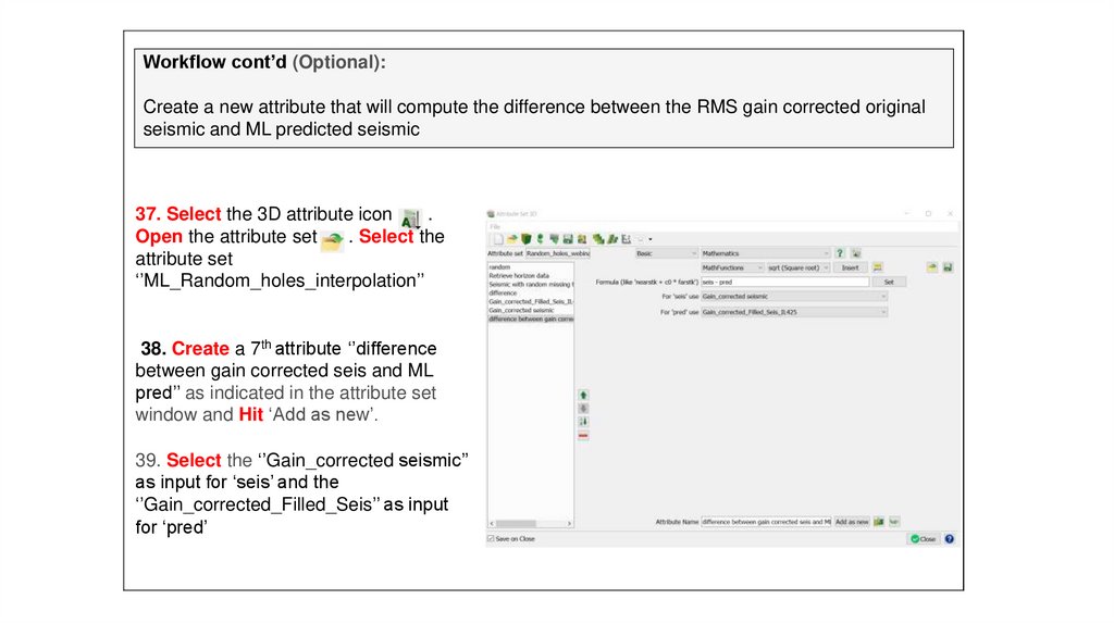
Workflow cont’d (Optional):Create a new attribute that will compute the difference between the RMS gain corrected original
seismic and ML predicted seismic
37. Select the 3D attribute icon
.
Open the attribute set
. Select the
attribute set
‘’ML_Random_holes_interpolation’’
38. Create a 7th attribute ‘’difference
between gain corrected seis and ML
pred’’ as indicated in the attribute set
window and Hit ‘Add as new’.
39. Select the ‘’Gain_corrected seismic’’
as input for ‘seis’ and the
‘’Gain_corrected_Filled_Seis’’ as input
for ‘pred’
22.
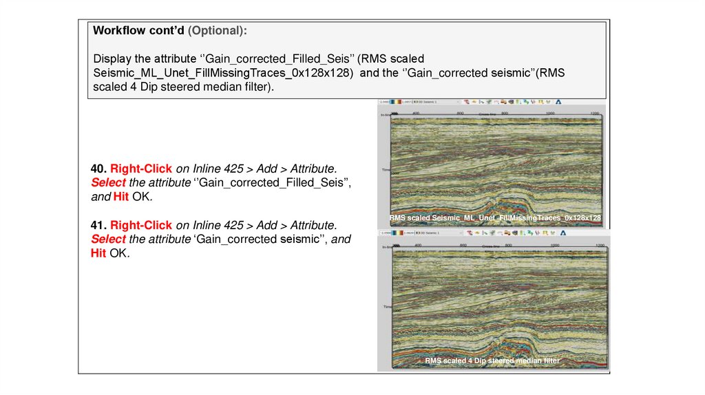
Workflow cont’d (Optional):Display the attribute ‘’Gain_corrected_Filled_Seis’’ (RMS scaled
Seismic_ML_Unet_FillMissingTraces_0x128x128) and the ‘’Gain_corrected seismic’’(RMS
scaled 4 Dip steered median filter).
40. Right-Click on Inline 425 > Add > Attribute.
Select the attribute ‘’Gain_corrected_Filled_Seis’’,
and Hit OK.
41. Right-Click on Inline 425 > Add > Attribute.
Select the attribute ‘Gain_corrected seismic’’, and
Hit OK.
RMS scaled Seismic_ML_Unet_FillMissingTraces_0x128x128
RMS scaled 4 Dip steered median filter
23.
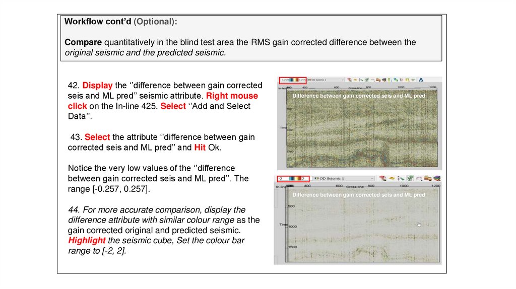
Workflow cont’d (Optional):Compare quantitatively in the blind test area the RMS gain corrected difference between the
original seismic and the predicted seismic.
42. Display the ‘’difference between gain corrected
seis and ML pred’’ seismic attribute. Right mouse
click on the In-line 425. Select ‘’Add and Select
Data’’.
Difference between gain corrected seis and ML pred
43. Select the attribute ‘’difference between gain
corrected seis and ML pred’’ and Hit Ok.
Notice the very low values of the ‘’difference
between gain corrected seis and ML pred’’. The
range [-0.257, 0.257].
44. For more accurate comparison, display the
difference attribute with similar colour range as the
gain corrected original and predicted seismic.
Highlight the seismic cube, Set the colour bar
range to [-2, 2].
Difference between gain corrected seis and ML pred