Model Parameterization in tomography problems. Lecture 4

1. Контрольные вопросы: 1. Суть линеаризации в задаче томографии. 2. Переход от интегралов к системе линейных уравнений в задаче

томографии.
3. Регуляризация (амплитудный демпинг,
сглаживание).

2.

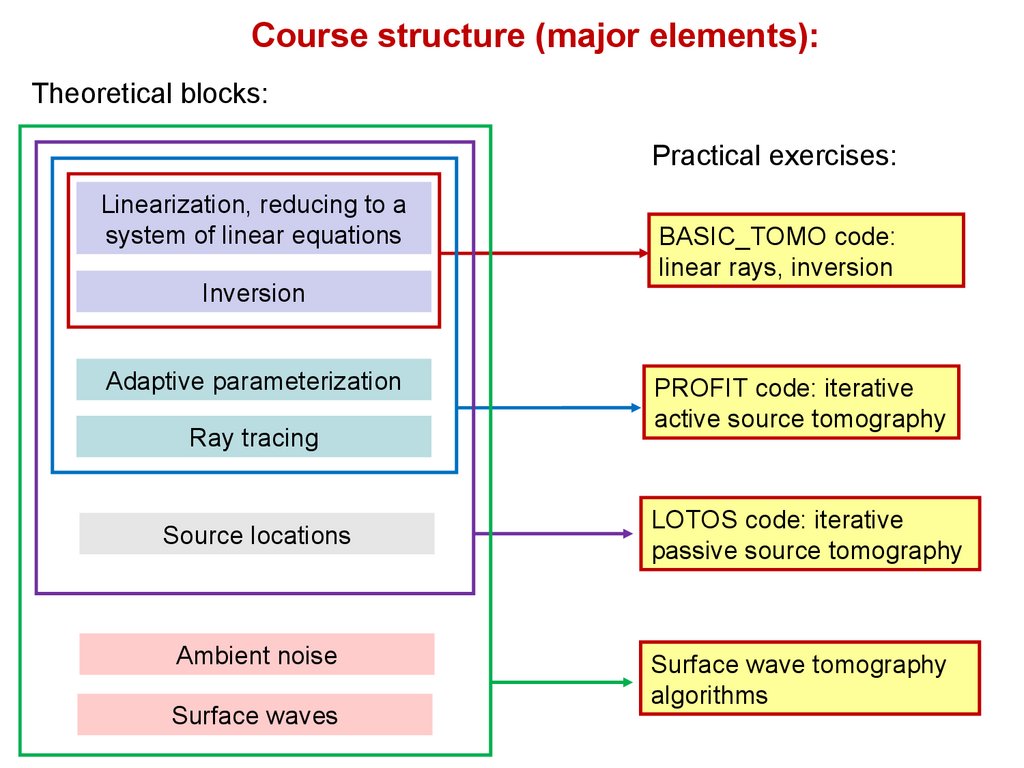
Course structure (major elements):
Theoretical blocks:
Practical exercises:
Linearization, reducing to a
system of linear equations
Inversion
Adaptive parameterization
Ray tracing
Source locations
Ambient noise
Surface waves
BASIC_TOMO code:
linear rays, inversion
PROFIT code: iterative
active source tomography
LOTOS code: iterative
passive source tomography
Surface wave tomography
algorithms

3. Lecture 4 Model Parameterization in tomography problems

Ivan Koulakov
IPGG

4.

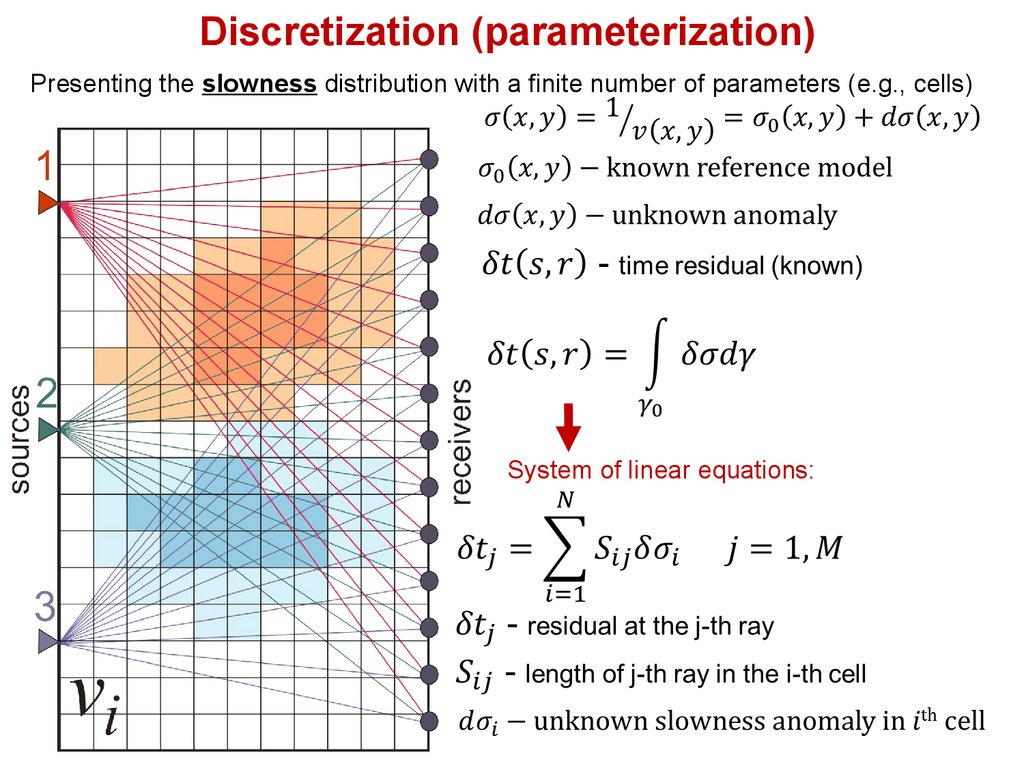
Discretization (parameterization)
Presenting the slowness distribution with a finite number of parameters (e.g., cells)
System of linear equations:

5.

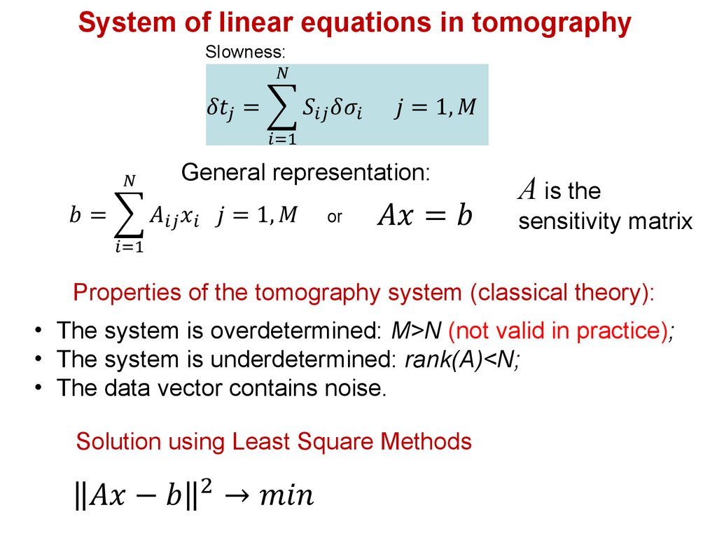
System of linear equations in tomography
Slowness:
General representation:
or
A is the
sensitivity matrix
Properties of the tomography system (classical theory):
• The system is overdetermined: M>N (not valid in practice);
• The system is underdetermined: rank(A)<N;
• The data vector contains noise.
Solution using Least Square Methods

6.

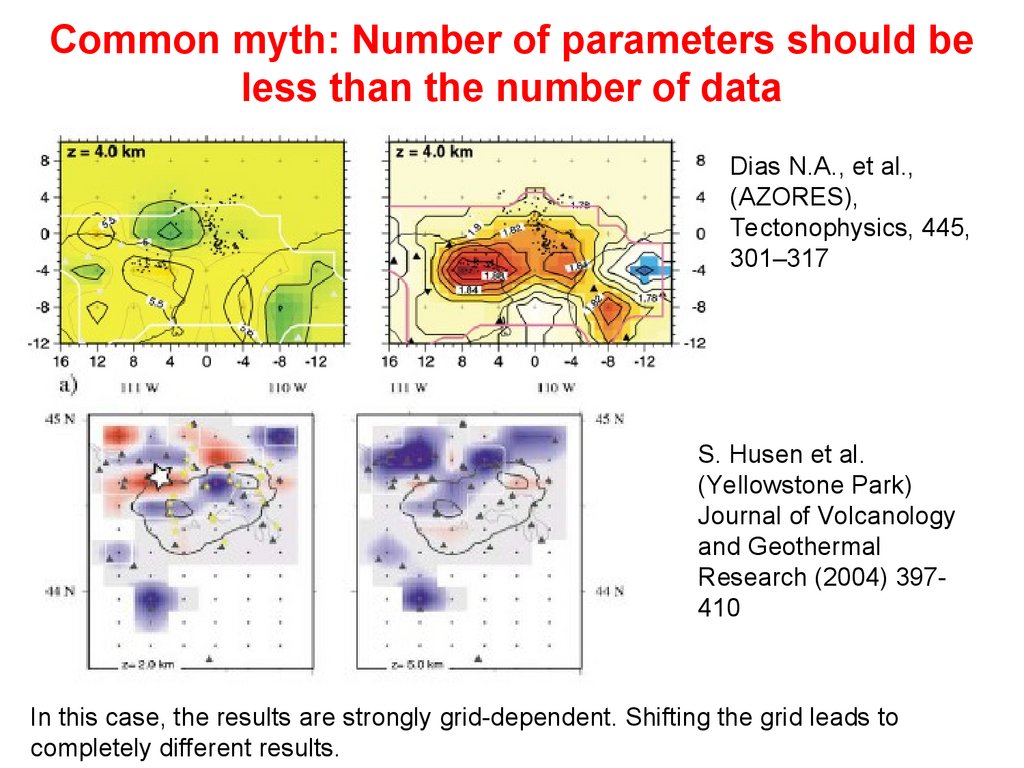
Common myth: Number of parameters should be
less than the number of data
Dias N.A., et al.,
(AZORES),
Tectonophysics, 445,
301–317
S. Husen et al.
(Yellowstone Park)
Journal of Volcanology
and Geothermal
Research (2004) 397410
In this case, the results are strongly grid-dependent. Shifting the grid leads to
completely different results.

7.

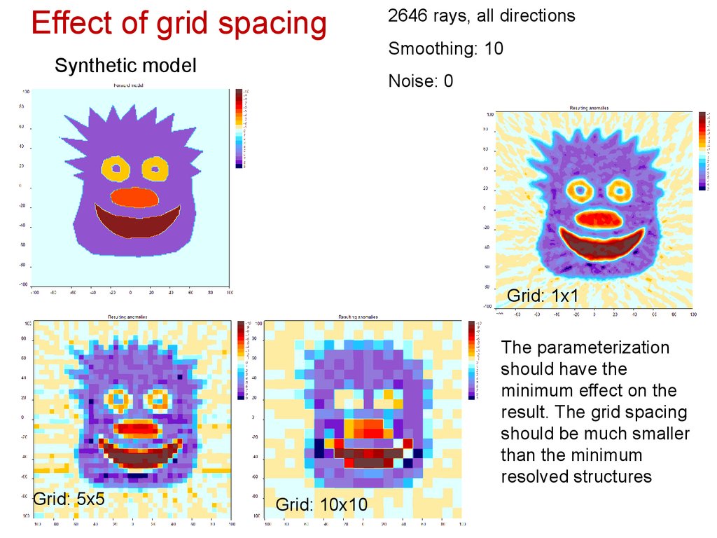
Effect of grid spacing
Synthetic model
2646 rays, all directions
Smoothing: 10
Noise: 0
Grid: 1x1
The parameterization
should have the
minimum effect on the
result. The grid spacing
should be much smaller
than the minimum
resolved structures
Grid: 5x5
Grid: 10x10

8.

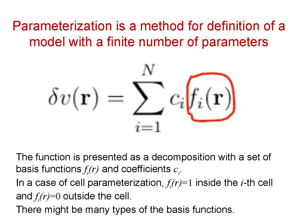
Parameterization is a method for definition of a
model with a finite number of parameters
The function is presented as a decomposition with a set of
basis functions fi(r) and coefficients ci.
In a case of cell parameterization, fi(r)=1 inside the i-th cell
and fi(r)=0 outside the cell.
There might be many types of the basis functions.

9.

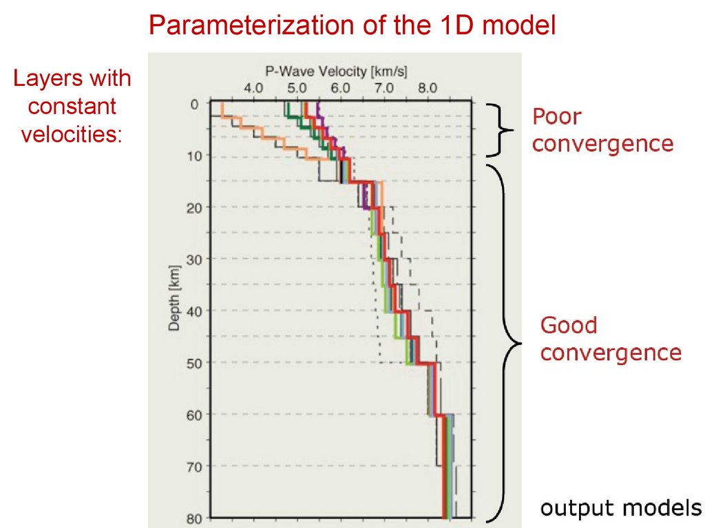
Parameterization of the 1D model
Layers with
constant
velocities:

10.

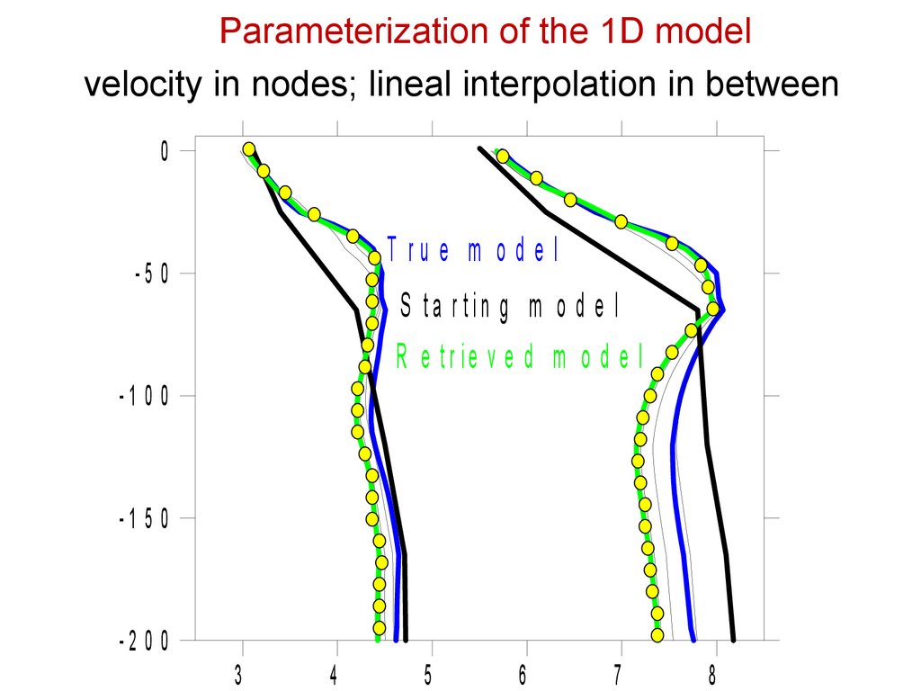
Parameterization of the 1D model
velocity in nodes; lineal interpolation in between
0
T ru e m o d e l
-5 0
S ta r tin g m o d e l
R e tr ie v e d m o d e l
-1 0 0
-1 5 0
-2 0 0
3
4
5
6
7
8

11.

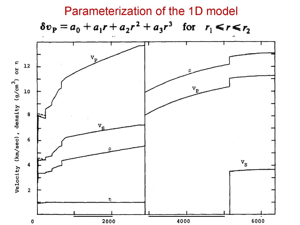
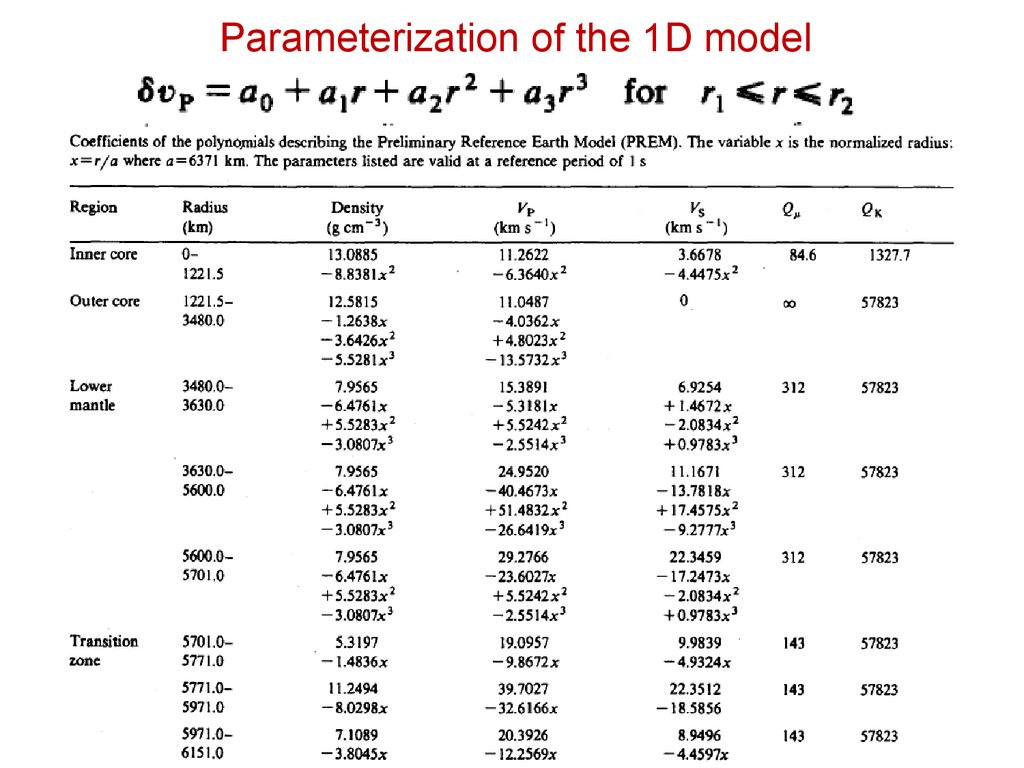
Parameterization of the 1D model
Coefficients of the Taylor series
(polynomes)

12.

Parameterization of the 1D model

13.

Parameterization of the 1D model

14.

Parameterization of the 1D model

15.

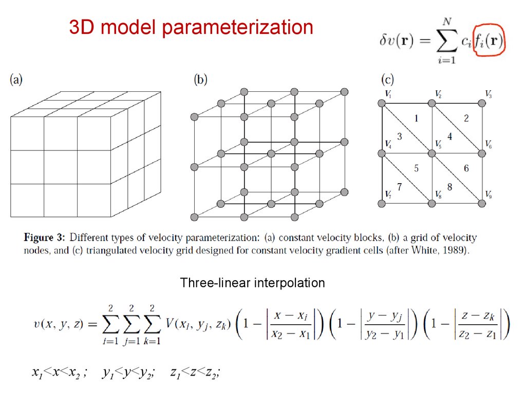
3D model parameterization
Three-linear interpolation
x1<x<x2 ;
y1<y<y2;
z1<z<z2;

16.

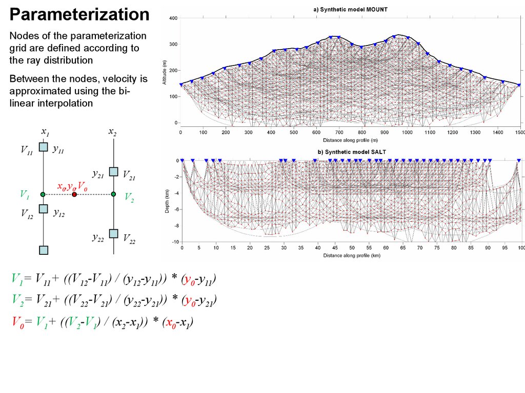
Parameterization
Nodes of the parameterization
grid are defined according to
the ray distribution
Between the nodes, velocity is
approximated using the bilinear interpolation
x2
x1
V11
y11
y21
V1
V12
x0,y0,V0
V21
V2
y12
y22
V22
V1= V11+ ((V12-V11) / (y12-y11)) * (y0-y11)
V2= V21+ ((V22-V21) / (y22-y21)) * (y0-y21)
V0= V1+ ((V2-V1) / (x2-x1)) * (x0-x1)

17.

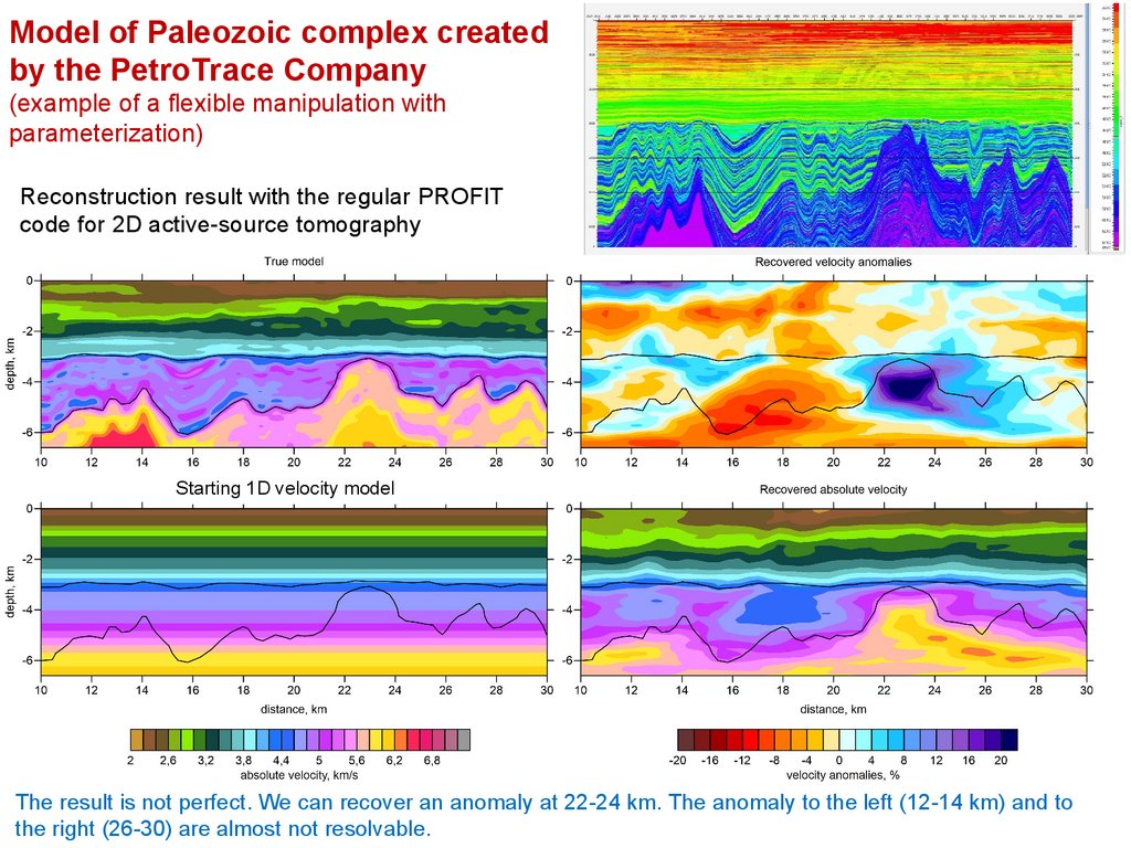
Model of Paleozoic complex created
by the PetroTrace Company
(example of a flexible manipulation with
parameterization)
Reconstruction result with the regular PROFIT
code for 2D active-source tomography
Starting 1D velocity model
The result is not perfect. We can recover an anomaly at 22-24 km. The anomaly to the left (12-14 km) and to
the right (26-30) are almost not resolvable.

18.

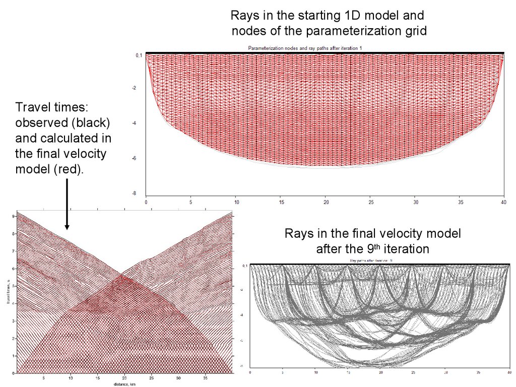
Rays in the starting 1D model and
nodes of the parameterization grid
Travel times:
observed (black)
and calculated in
the final velocity
model (red).
Rays in the final velocity model
after the 9th iteration

19.

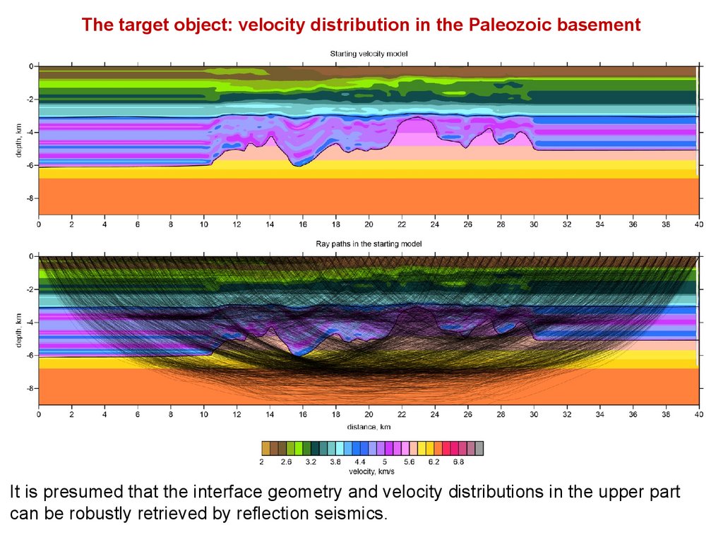
The target object: velocity distribution in the Paleozoic basement
It is presumed that the interface geometry and velocity distributions in the upper part
can be robustly retrieved by reflection seismics.

20.

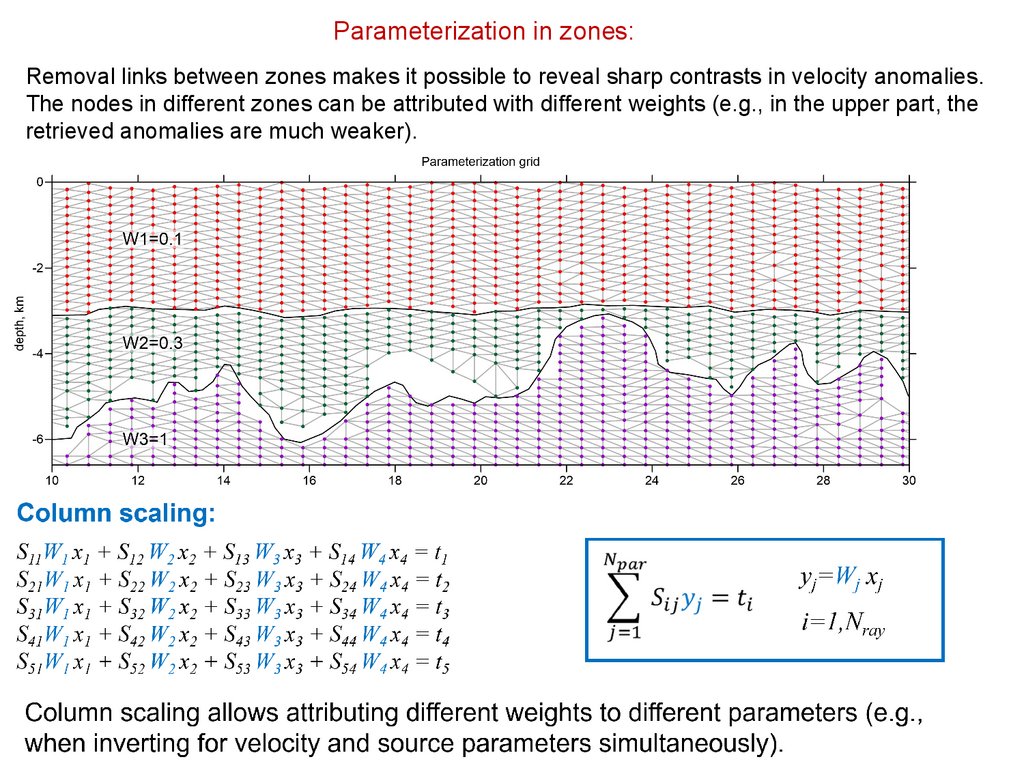
Parameterization in zones:
Removal links between zones makes it possible to reveal sharp contrasts in velocity anomalies.
The nodes in different zones can be attributed with different weights (e.g., in the upper part, the
retrieved anomalies are much weaker).

21.

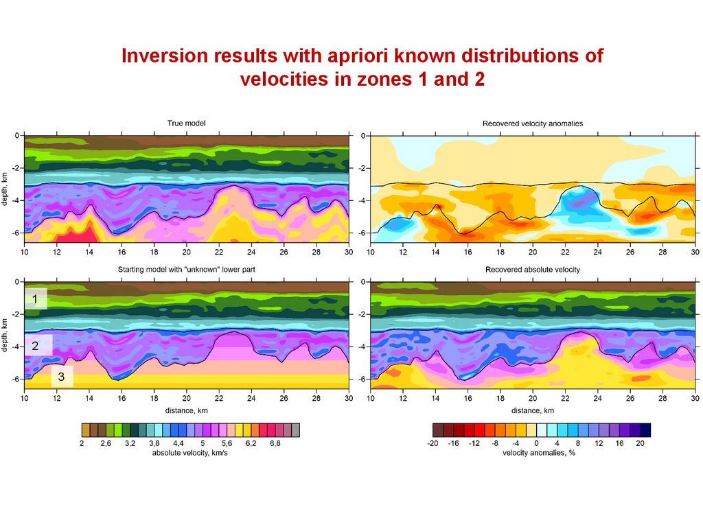
Inversion results with apriori known distributions of
velocities in zones 1 and 2
1
2
3

22.

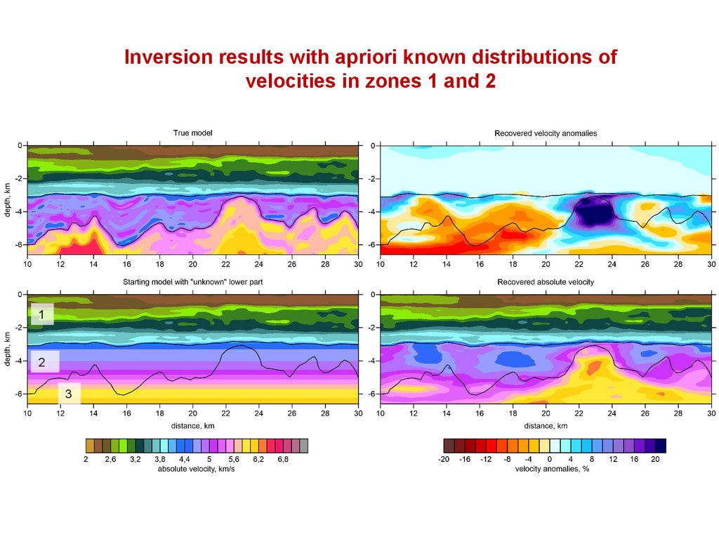
Inversion results with apriori known distributions of
velocities in zones 1 and 2
1
2
3

23.

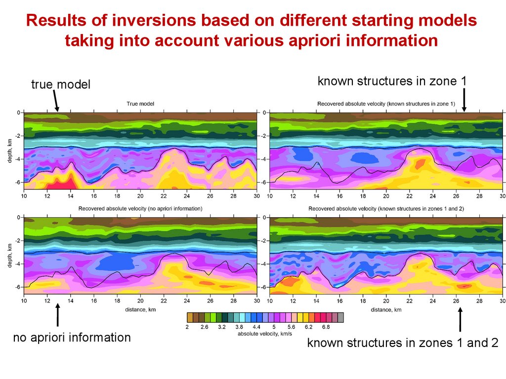
Results of inversions based on different starting models
taking into account various apriori information
true model
no apriori information
known structures in zone 1
known structures in zones 1 and 2

24.

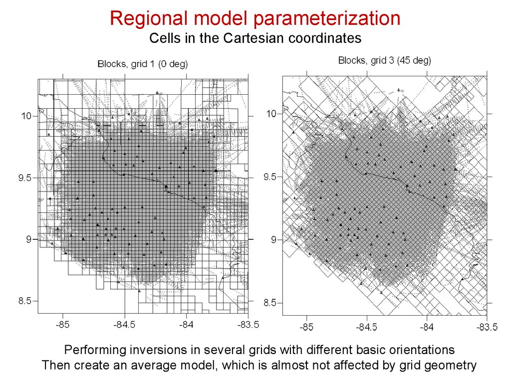
Regional model parameterization
Cells in the Cartesian coordinates
Performing inversions in several grids with different basic orientations
Then create an average model, which is almost not affected by grid geometry

25.

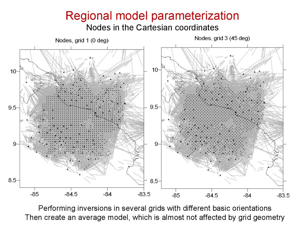
Regional model parameterization
Nodes in the Cartesian coordinates
Performing inversions in several grids with different basic orientations
Then create an average model, which is almost not affected by grid geometry

26.

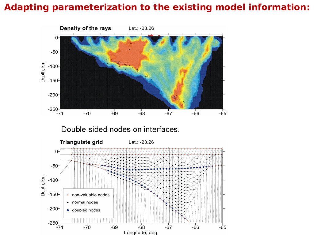
Adapting parameterization to the existing model information:
Double-sided nodes on interfaces.

27.

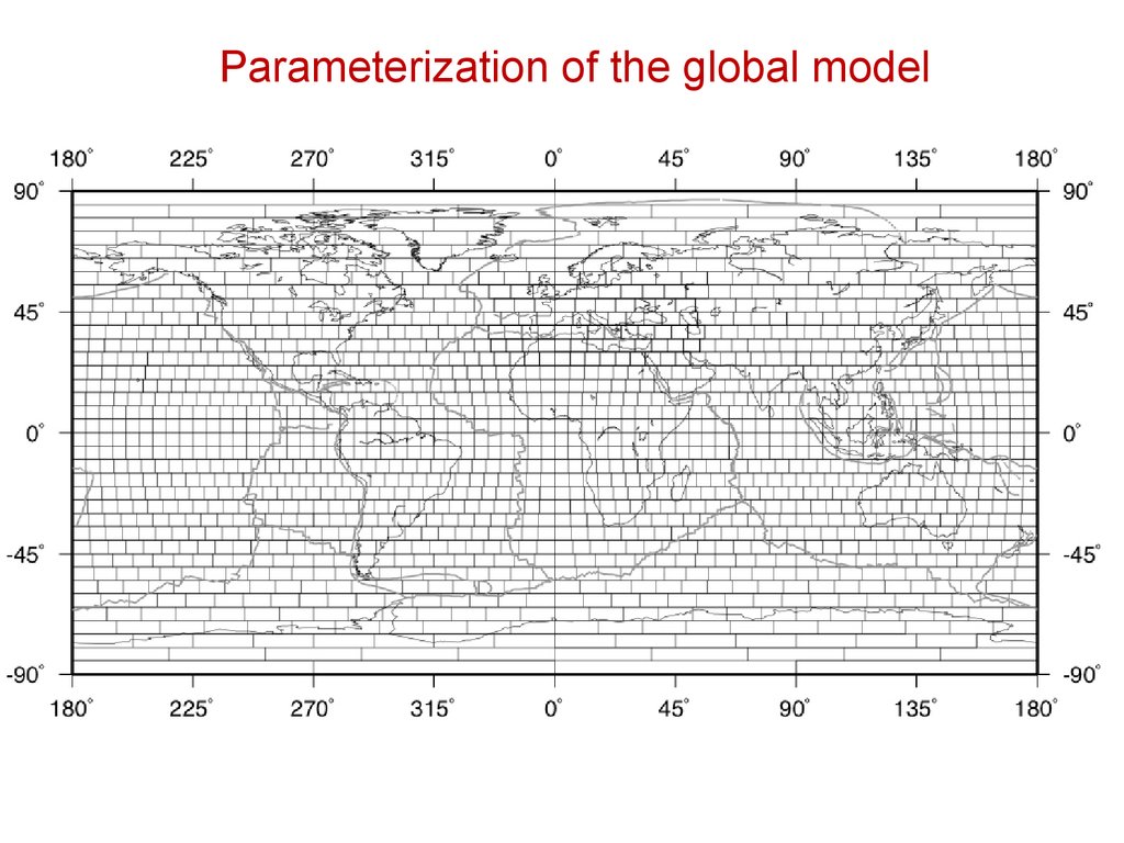
Parameterization of the global model

28.

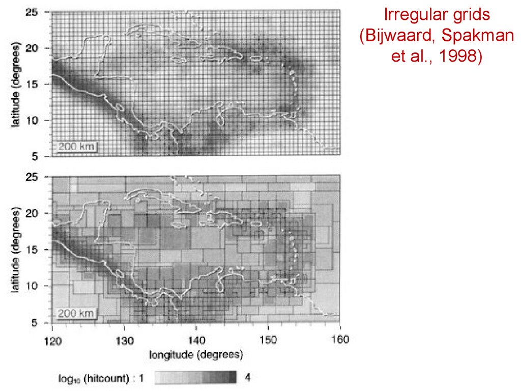
Irregular grids
(Bijwaard, Spakman
et al., 1998)

29.

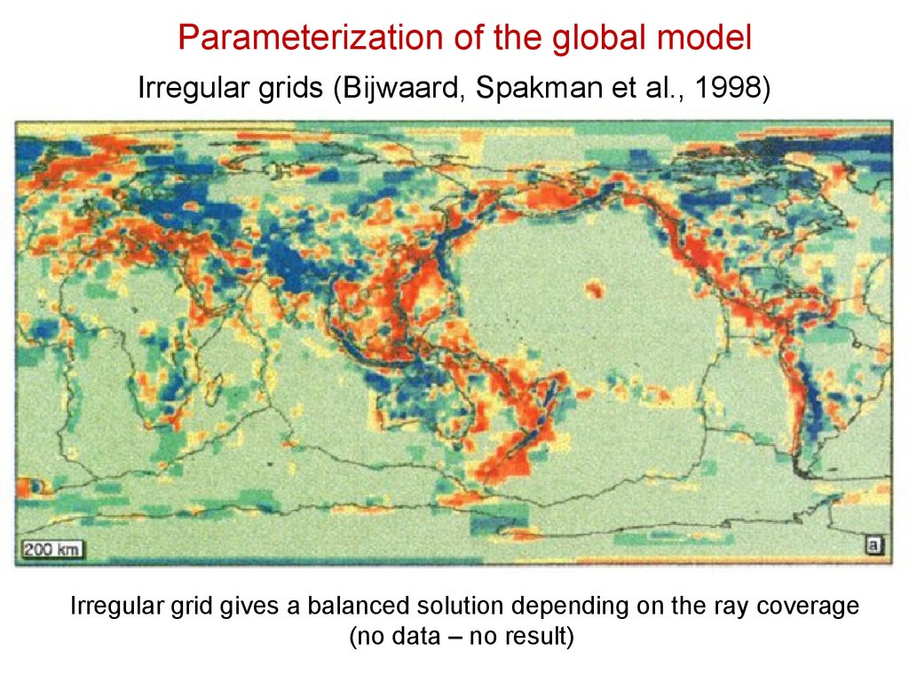
Parameterization of the global model
Irregular grids (Bijwaard, Spakman et al., 1998)
Irregular grid gives a balanced solution depending on the ray coverage
(no data – no result)

30.

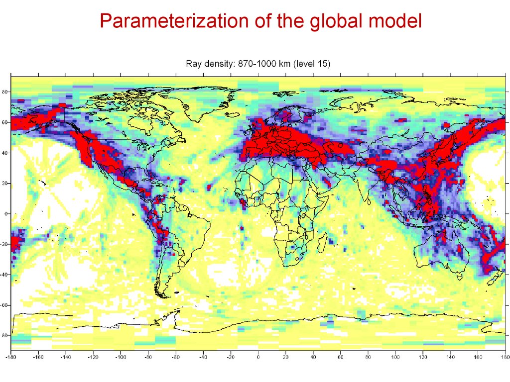
Parameterization of the global model

31.

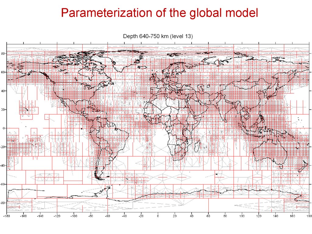
Parameterization of the global model

32.

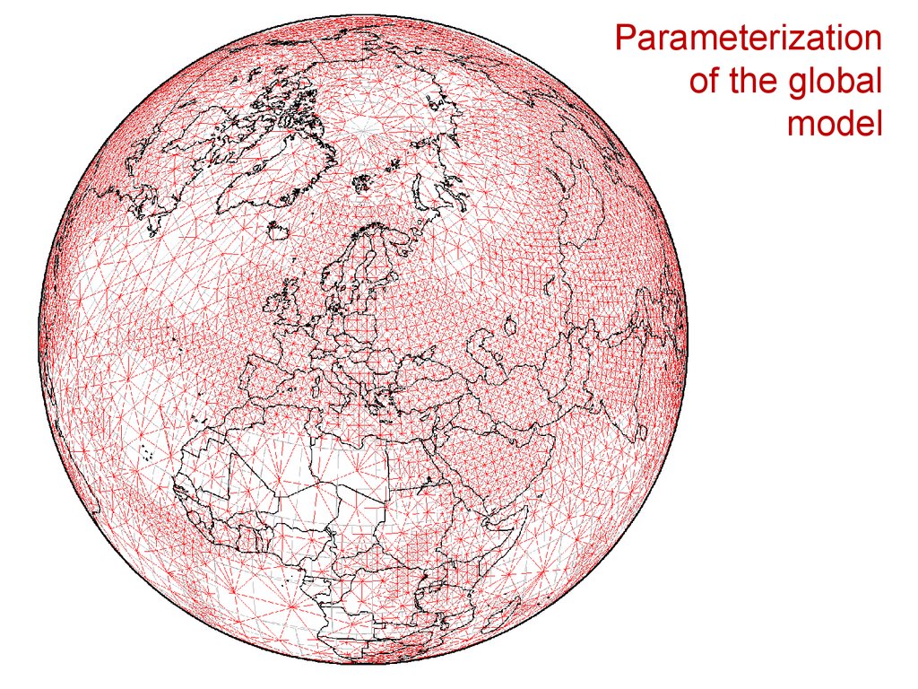
Parameterization
of the global
model

33.

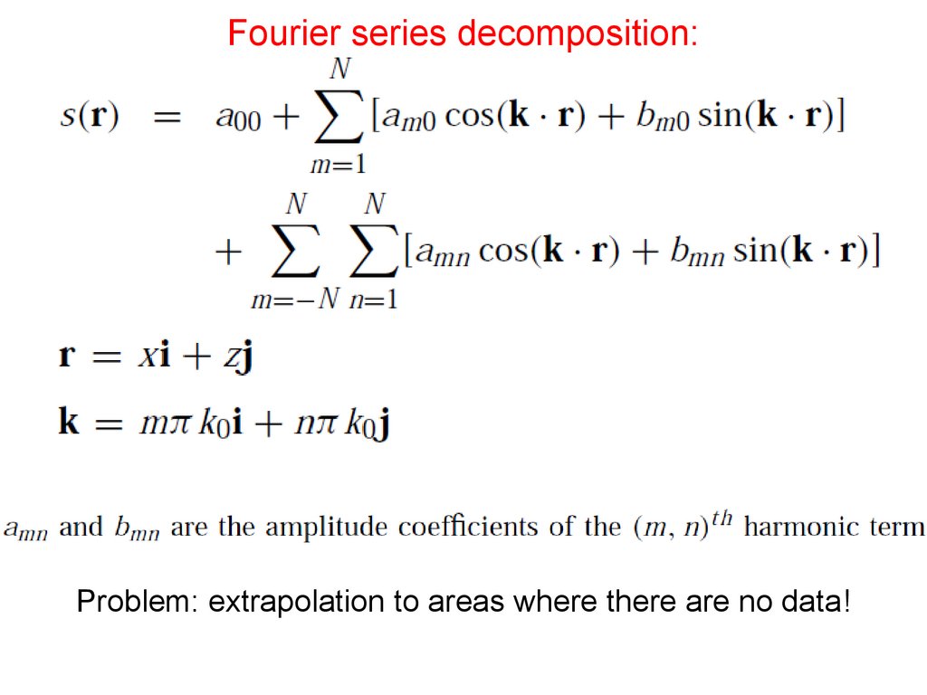
Fourier series decomposition:
Problem: extrapolation to areas where there are no data!

34.

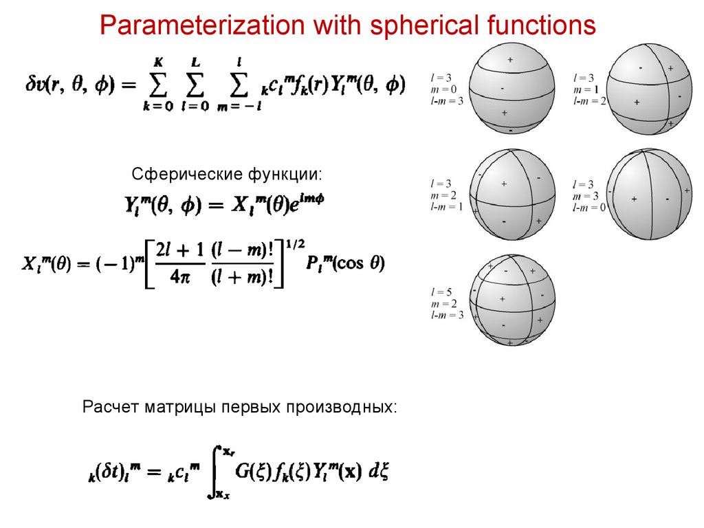
Parameterization with spherical functions
Сферические функции:
Расчет матрицы первых производных:

35.

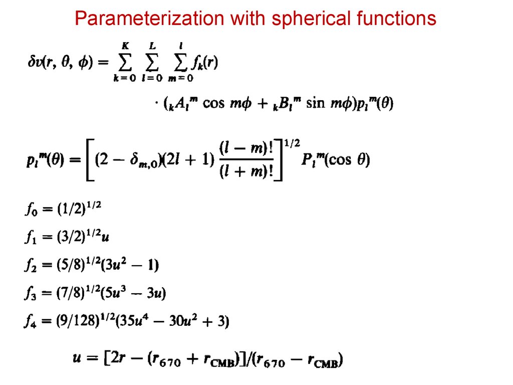
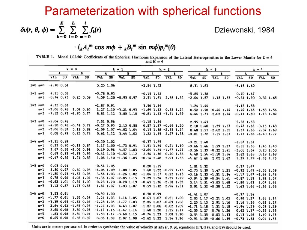
Parameterization with spherical functions

36.

Parameterization with spherical functions
Dziewonski, 1984

37. The properties of a “super-red” spectrum

harmonic order
15 times more coefficients