Similar presentations:
Solution Methods Applied Computational Fluid Dynamics. Lecture 5
1. Lecture 5 - Solution Methods Applied Computational Fluid Dynamics
Instructor: André Bakker© André Bakker (2002-2005)
© Fluent Inc. (2002)
1
2. Solution methods
Focus on finite volume method.
Background of finite volume method.
Discretization example.
General solution method.
Convergence.
Accuracy and numerical diffusion.
Pressure velocity coupling.
Segregated versus coupled solver methods.
Multigrid solver.
Summary.
2
3. Overview of numerical methods
• Many CFD techniques exist.• The most common in commercially available CFD programs are:
– The finite volume method has the broadest applicability (~80%).
– Finite element (~15%).
• Here we will focus on the finite volume method.
• There are certainly many other approaches (5%), including:
–
–
–
–
–
–
–
Finite difference.
Finite element.
Spectral methods.
Boundary element.
Vorticity based methods.
Lattice gas/lattice Boltzmann.
And more!
3
4. Finite difference method (FDM)
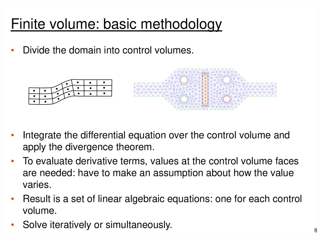
Finite volume: basic methodology• Divide the domain into control volumes.
•
• •
• •
• Integrate the differential equation over the control volume and
apply the divergence theorem.
• To evaluate derivative terms, values at the control volume faces
are needed: have to make an assumption about how the value
varies.
• Result is a set of linear algebraic equations: one for each control
volume.
• Solve iteratively or simultaneously.
8
5. Finite difference: basic methodology
Cells and nodes• Using finite volume method, the solution domain is subdivided
into a finite number of small control volumes (cells) by a grid.
• The grid defines the boundaries of the control volumes while the
computational node lies at the center of the control volume.
• The advantage of FVM is that the integral conservation is
satisfied exactly over the control volume.
Boundary node
Control volume
Computational node
9
6. Finite element method (FEM)
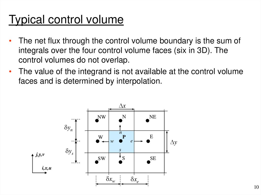
Typical control volume• The net flux through the control volume boundary is the sum of
integrals over the four control volume faces (six in 3D). The
control volumes do not overlap.
• The value of the integrand is not available at the control volume
faces and is determined by interpolation.
Dx
N
NW
dyn
n
W
j,y,v
NE
P
w
dys
e
E
Dy
s
S
SW
SE
i,x,u
dxw
dxe
10
7. Finite volume method (FVM)
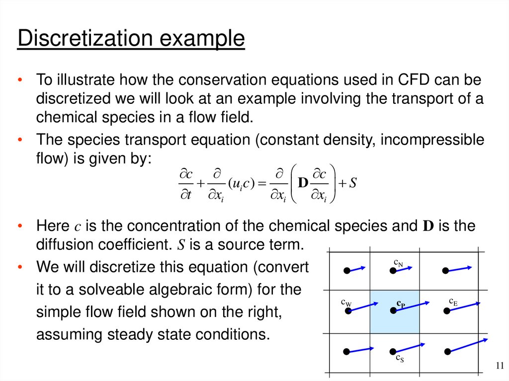
Discretization example• To illustrate how the conservation equations used in CFD can be
discretized we will look at an example involving the transport of a
chemical species in a flow field.
• The species transport equation (constant density, incompressible
flow) is given by:
c
c
(ui c)
D
S
t xi
xi xi
• Here c is the concentration of the chemical species and D is the
diffusion coefficient. S is a source term.
cN
• We will discretize this equation (convert
it to a solveable algebraic form) for the
cE
cW
cP
simple flow field shown on the right,
assuming steady state conditions.
cS
11
8. Finite volume: basic methodology
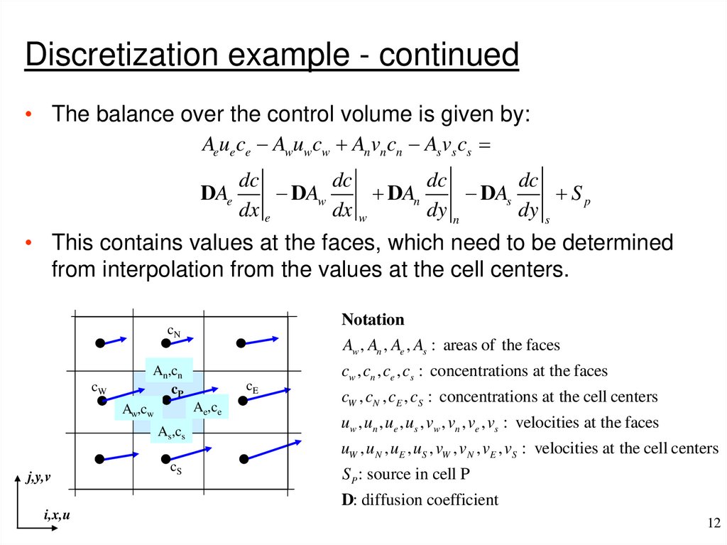
Discretization example - continued• The balance over the control volume is given by:
Aeue ce Awuwcw An vn cn As vs cs
DAe
dc
dc
dc
dc
DAw
DAn
DAs
Sp
dx e
dx w
dy n
dy s
• This contains values at the faces, which need to be determined
from interpolation from the values at the cell centers.
Notation
cN
cW
Aw , An , Ae , As : areas of the faces
An,cn
cP
cE
Ae,ce
Aw,cw
As,cs
cw , cn , ce , cs : concentrations at the faces
cW , cN , cE , cS : concentrations at the cell centers
uw , un , ue , us , vw , vn , ve , vs : velocities at the faces
uW , u N , uE , uS , vW , vN , vE , vS : velocities at the cell centers
j,y,v
cS
S P : source in cell P
D: diffusion coefficient
i,x,u
12
9. Cells and nodes
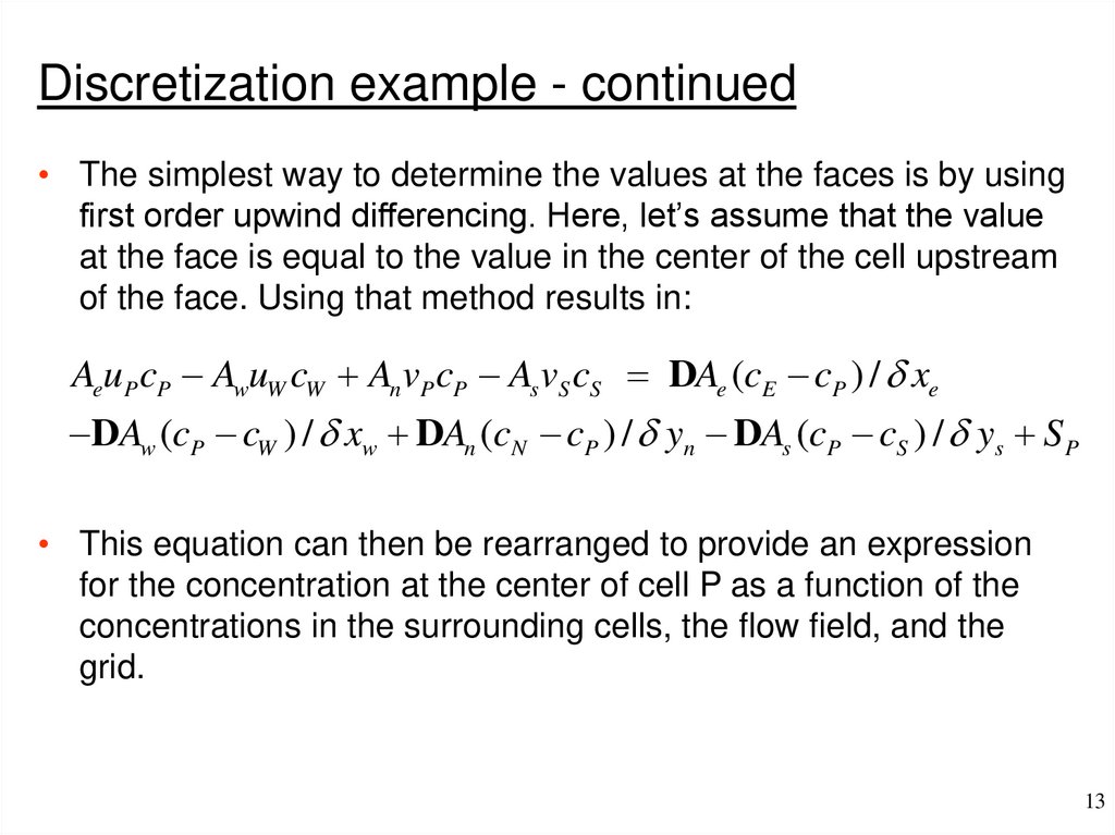
Discretization example - continued• The simplest way to determine the values at the faces is by using
first order upwind differencing. Here, let’s assume that the value
at the face is equal to the value in the center of the cell upstream
of the face. Using that method results in:
AeuP cP AwuW cW An vP cP As vS cS DAe (cE cP ) / d xe
DAw (cP cW ) / d xw DAn (cN cP ) / d yn DAs (cP cS ) / d ys S P
• This equation can then be rearranged to provide an expression
for the concentration at the center of cell P as a function of the
concentrations in the surrounding cells, the flow field, and the
grid.
13
10. Typical control volume
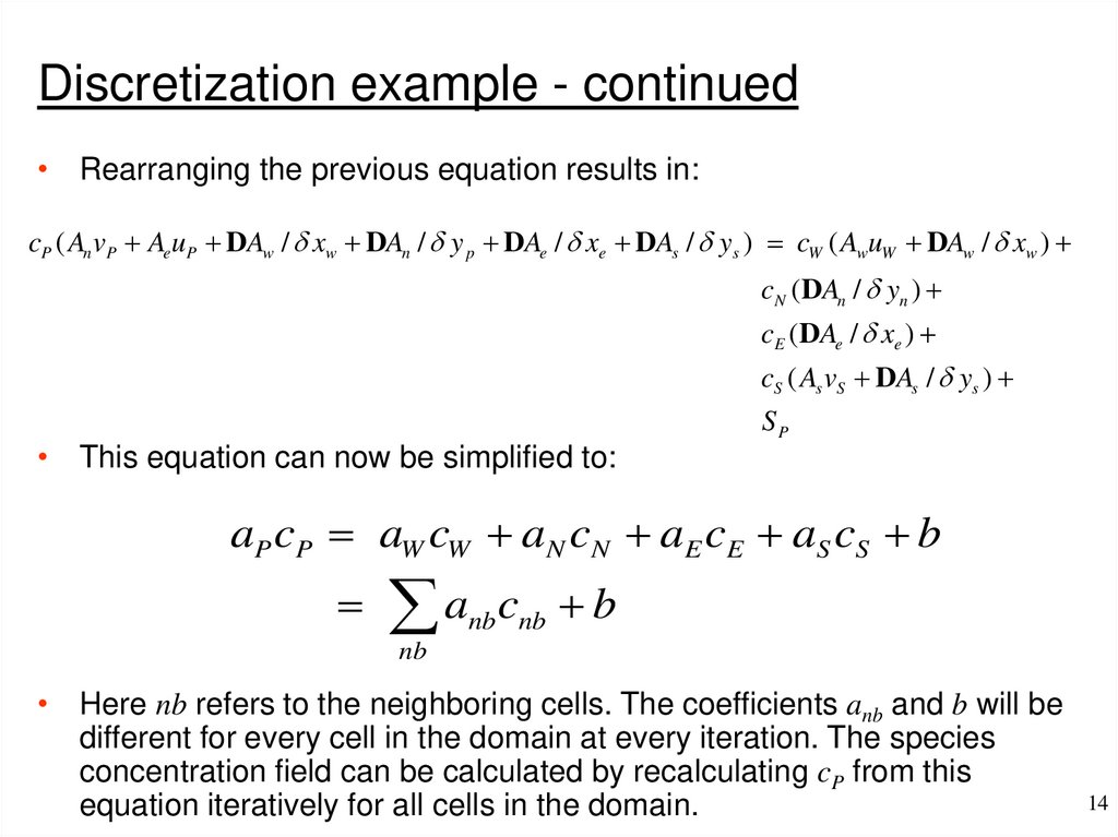
Discretization example - continued• Rearranging the previous equation results in:
cP ( An vP AeuP DAw / d xw DAn / d y p DAe / d xe DAs / d ys ) cW ( AwuW DAw / d xw )
cN (DAn / d yn )
cE (DAe / d xe )
cS ( As vS DAs / d ys )
• This equation can now be simplified to:
SP
aP cP aW cW aN cN aE cE aS cS b
a
c b
nb nb
nb
• Here nb refers to the neighboring cells. The coefficients anb and b will be
different for every cell in the domain at every iteration. The species
concentration field can be calculated by recalculating cP from this
equation iteratively for all cells in the domain.
14
11. Discretization example
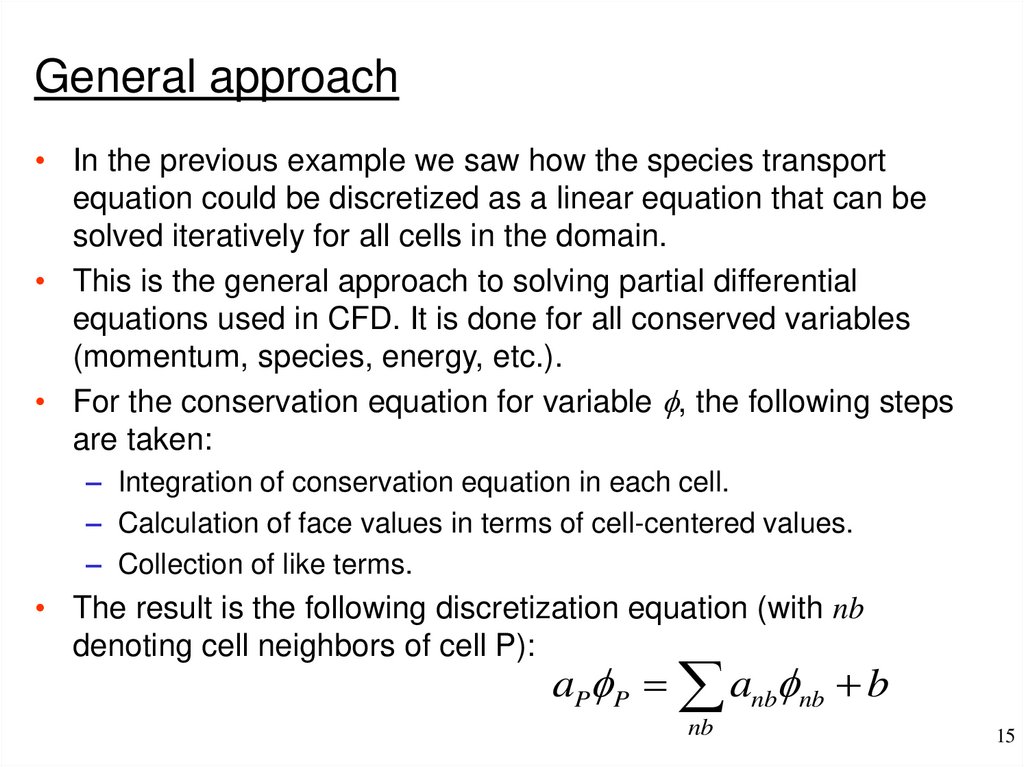
General approach• In the previous example we saw how the species transport
equation could be discretized as a linear equation that can be
solved iteratively for all cells in the domain.
• This is the general approach to solving partial differential
equations used in CFD. It is done for all conserved variables
(momentum, species, energy, etc.).
• For the conservation equation for variable f, the following steps
are taken:
– Integration of conservation equation in each cell.
– Calculation of face values in terms of cell-centered values.
– Collection of like terms.
• The result is the following discretization equation (with nb
denoting cell neighbors of cell P):
aPfP anbfnb b
nb
15
12. Discretization example - continued
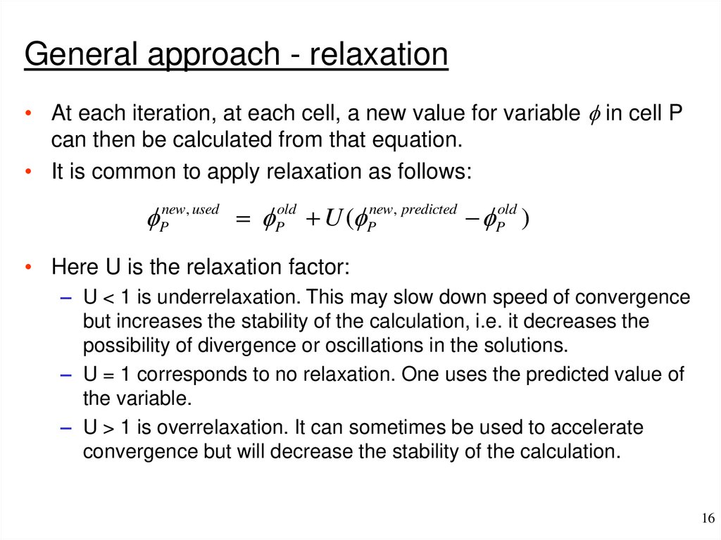
General approach - relaxation• At each iteration, at each cell, a new value for variable f in cell P
can then be calculated from that equation.
• It is common to apply relaxation as follows:
fPnew, used fPold U (fPnew, predicted fPold )
• Here U is the relaxation factor:
– U < 1 is underrelaxation. This may slow down speed of convergence
but increases the stability of the calculation, i.e. it decreases the
possibility of divergence or oscillations in the solutions.
– U = 1 corresponds to no relaxation. One uses the predicted value of
the variable.
– U > 1 is overrelaxation. It can sometimes be used to accelerate
convergence but will decrease the stability of the calculation.
16
13. Discretization example - continued
Underrelaxation recommendation• Underrelaxation factors are there to suppress oscillations in the
flow solution that result from numerical errors.
• Underrelaxation factors that are too small will significantly slow
down convergence, sometimes to the extent that the user thinks
the solution is converged when it really is not.
• The recommendation is to always use underrelaxation factors
that are as high as possible, without resulting in oscillations or
divergence.
• Typically one should stay with the default factors in the solver.
• When the solution is converged but the pressure residual is still
relatively high, the factors for pressure and momentum can be
lowered to further refine the solution.
17
14. Discretization example - continued
General approach - convergence• The iterative process is repeated until the change in the variable
from one iteration to the next becomes so small that the solution
can be considered converged.
• At convergence:
– All discrete conservation equations (momentum, energy, etc.) are
obeyed in all cells to a specified tolerance.
– The solution no longer changes with additional iterations.
– Mass, momentum, energy and scalar balances are obtained.
• Residuals measure imbalance (or error) in conservation
equations.
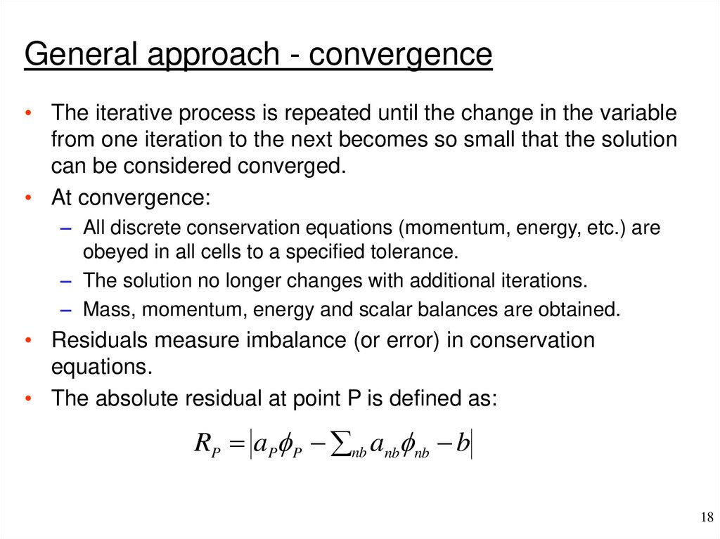
• The absolute residual at point P is defined as:
RP aPf P nb anbfnb b
18
15. General approach
Convergence - continued• Residuals are usually scaled relative to the local value of the
property f in order to obtain a relative error:
RP , scaled
a Pf P nb anbf nb b
a Pf P
• They can also be normalized, by dividing them by the maximum
residual that was found at any time during the iterative process.
• An overall measure of the residual in the domain is:
aPf P nb anbf nb b
Rf all cells
aPf P
all cells
• It is common to require the scaled residuals to be on the order of
1E-3 to 1E-4 or less for convergence.
19
16. General approach - relaxation
Notes on convergence• Always ensure proper convergence before using a solution:
unconverged solutions can be misleading!!
• Solutions are converged when the flow field and scalar fields are
no longer changing.
• Determining when this is the case can be difficult.
• It is most common to monitor the residuals.
20
17. Underrelaxation recommendation
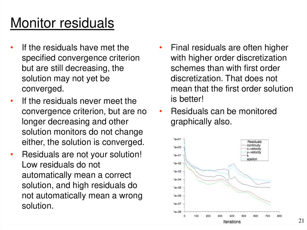
Monitor residuals• If the residuals have met the
specified convergence criterion
but are still decreasing, the
solution may not yet be
converged.
• If the residuals never meet the
convergence criterion, but are no
longer decreasing and other
solution monitors do not change
either, the solution is converged.
• Residuals are not your solution!
Low residuals do not
automatically mean a correct
solution, and high residuals do
not automatically mean a wrong
solution.
• Final residuals are often higher
with higher order discretization
schemes than with first order
discretization. That does not
mean that the first order solution
is better!
• Residuals can be monitored
graphically also.
21
18. General approach - convergence
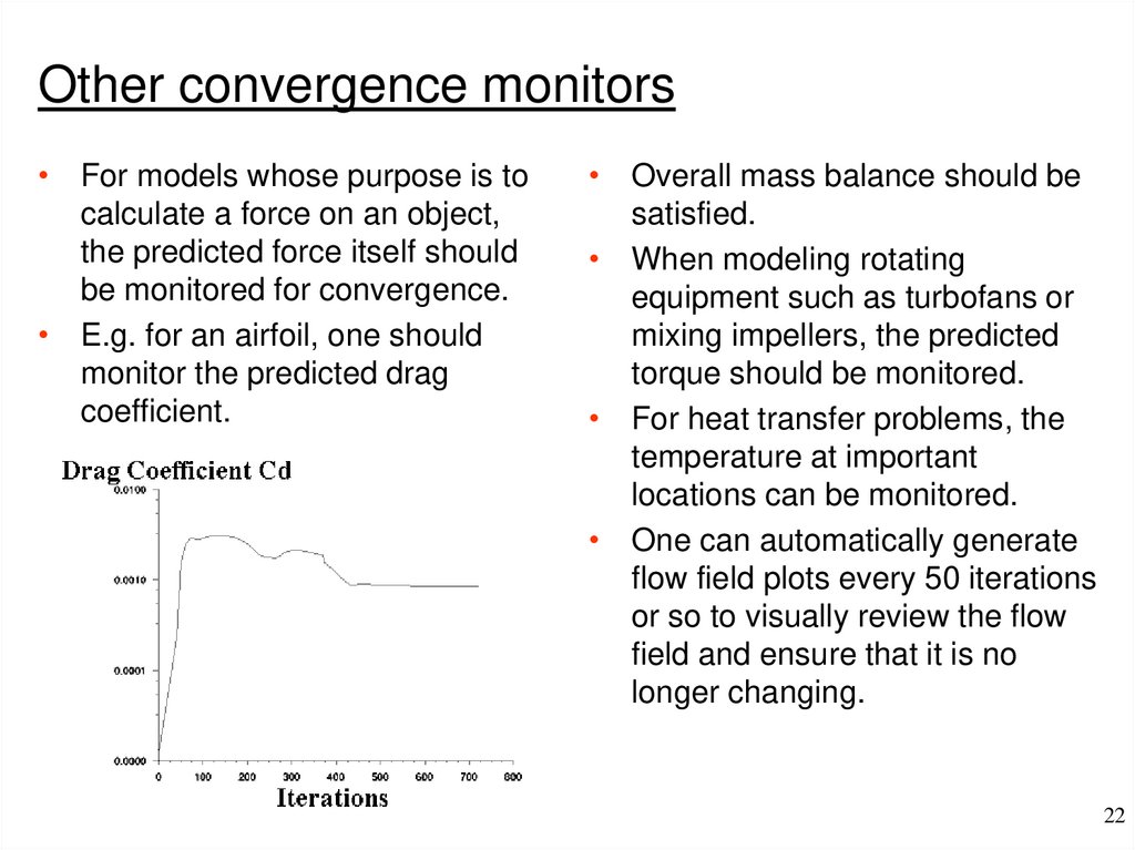
Other convergence monitors• For models whose purpose is to
calculate a force on an object,
the predicted force itself should
be monitored for convergence.
• E.g. for an airfoil, one should
monitor the predicted drag
coefficient.
• Overall mass balance should be
satisfied.
• When modeling rotating
equipment such as turbofans or
mixing impellers, the predicted
torque should be monitored.
• For heat transfer problems, the
temperature at important
locations can be monitored.
• One can automatically generate
flow field plots every 50 iterations
or so to visually review the flow
field and ensure that it is no
longer changing.
22
19. Convergence - continued
Numerical schemes: finding face values• Face values of f and f/ x are found by making assumptions
about variation of f between cell centers.
• Number of different schemes can be devised:
–
–
–
–
–
First-order upwind scheme.
Central differencing scheme.
Power-law scheme.
Second-order upwind scheme.
QUICK scheme.
• We will discuss these one by one.
23
20. Notes on convergence
First order upwind scheme• This is the simplest numerical
scheme. It is the method that we
used earlier in the discretization
example.
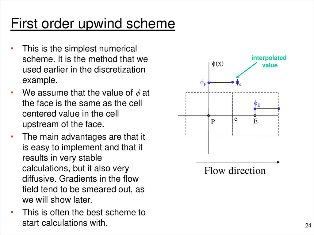
• We assume that the value of f at
the face is the same as the cell
centered value in the cell
upstream of the face.
• The main advantages are that it
is easy to implement and that it
results in very stable
calculations, but it also very
diffusive. Gradients in the flow
field tend to be smeared out, as
we will show later.
• This is often the best scheme to
start calculations with.
interpolated
value
f(x)
fe
fP
fE
P
e
E
Flow direction
24
21. Monitor residuals
Central differencing scheme• We determine the value of f at
the face by linear interpolation
between the cell centered
values.
• This is more accurate than the
first order upwind scheme, but it
leads to oscillations in the
solution or divergence if the local
Peclet number is larger than 2.
The Peclet number is the ratio
between convective and diffusive
uL
transport:
Pe
interpolated
value
f(x)
fP
fe
P
e
fE
E
D
• It is common to then switch to
first order upwind in cells where
Pe>2. Such an approach is
called a hybrid scheme.
25
22. Other convergence monitors
Power law scheme• This is based on the analytical
solution of the one-dimensional
convection-diffusion equation.
• The face value is determined
from an exponential profile
through the cell values. The
exponential profile is
approximated by the following
power law equation:
fe f P
1 0.1Pe 5
Pe
fE fP
• Pe is again the Peclet number.
• For Pe>10, diffusion is ignored
and first order upwind is used.
f(x)
interpolated
value
fP
fe
e
P
fE
E
x
L
26
23. Numerical schemes: finding face values
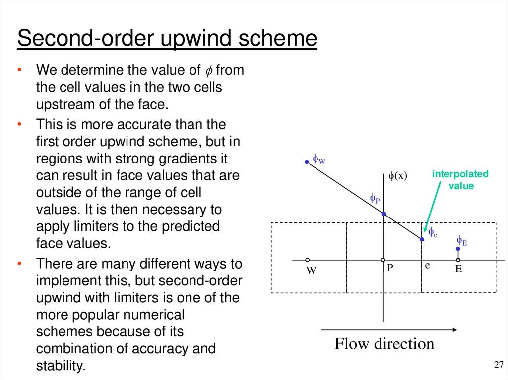
Second-order upwind scheme• We determine the value of f from
the cell values in the two cells
upstream of the face.
• This is more accurate than the
first order upwind scheme, but in
regions with strong gradients it
can result in face values that are
outside of the range of cell
values. It is then necessary to
apply limiters to the predicted
face values.
• There are many different ways to
implement this, but second-order
upwind with limiters is one of the
more popular numerical
schemes because of its
combination of accuracy and
stability.
fW
f(x)
interpolated
value
fP
fe
W
P
e
fE
E
Flow direction
27
24. First order upwind scheme
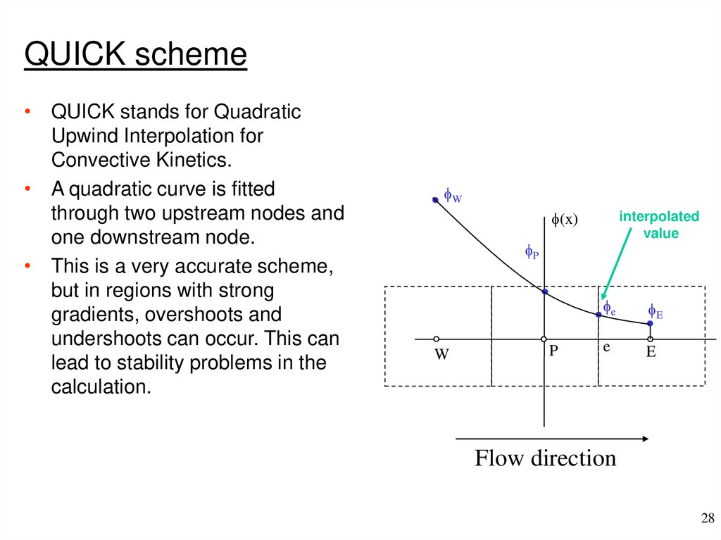
QUICK scheme• QUICK stands for Quadratic
Upwind Interpolation for
Convective Kinetics.
• A quadratic curve is fitted
through two upstream nodes and
one downstream node.
• This is a very accurate scheme,
but in regions with strong
gradients, overshoots and
undershoots can occur. This can
lead to stability problems in the
calculation.
fW
f(x)
interpolated
value
fP
W
P
fe
fE
e
E
Flow direction
28
25. Central differencing scheme
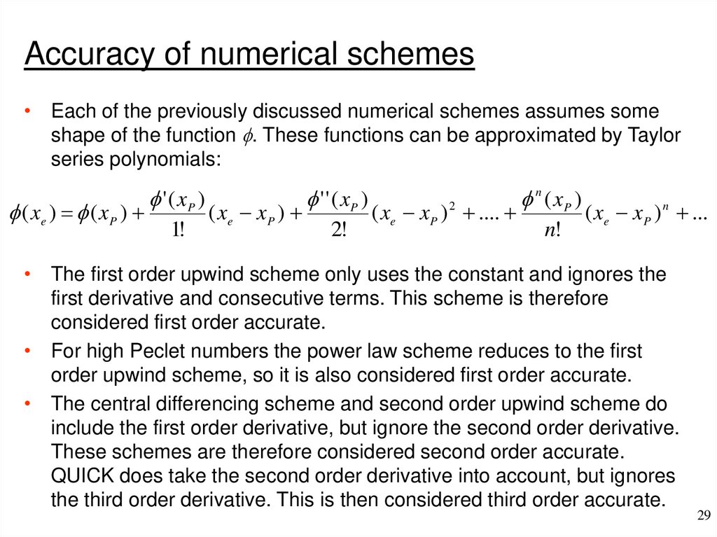
Accuracy of numerical schemes• Each of the previously discussed numerical schemes assumes some
shape of the function f. These functions can be approximated by Taylor
series polynomials:
f ( xe ) f ( x P )
f ' ( xP )
1!
( xe x P )
f ' ' ( xP )
2!
( xe xP ) ....
2
f n ( xP )
n!
( xe xP ) n ...
• The first order upwind scheme only uses the constant and ignores the
first derivative and consecutive terms. This scheme is therefore
considered first order accurate.
• For high Peclet numbers the power law scheme reduces to the first
order upwind scheme, so it is also considered first order accurate.
• The central differencing scheme and second order upwind scheme do
include the first order derivative, but ignore the second order derivative.
These schemes are therefore considered second order accurate.
QUICK does take the second order derivative into account, but ignores
the third order derivative. This is then considered third order accurate.
29
26. Power law scheme
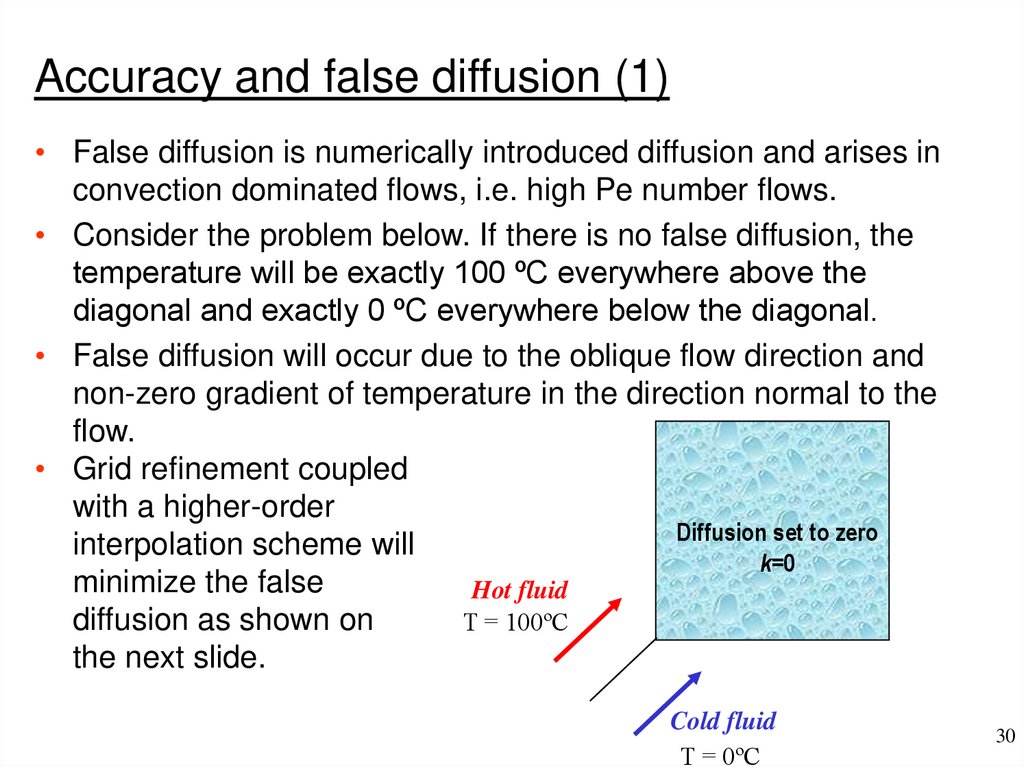
Accuracy and false diffusion (1)• False diffusion is numerically introduced diffusion and arises in
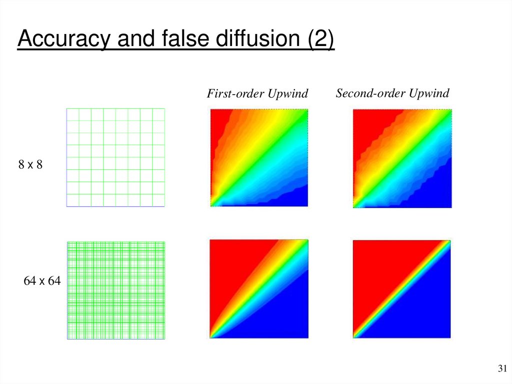
convection dominated flows, i.e. high Pe number flows.
• Consider the problem below. If there is no false diffusion, the
temperature will be exactly 100 ºC everywhere above the
diagonal and exactly 0 ºC everywhere below the diagonal.
• False diffusion will occur due to the oblique flow direction and
non-zero gradient of temperature in the direction normal to the
flow.
• Grid refinement coupled
with a higher-order
Diffusion set to zero
interpolation scheme will
k=0
minimize the false
Hot fluid
diffusion as shown on
T = 100ºC
the next slide.
Cold fluid
T = 0ºC
30
27. Second-order upwind scheme
Accuracy and false diffusion (2)First-order Upwind
Second-order Upwind
8x8
64 x 64
31
28. QUICK scheme
Properties of numerical schemes• All numerical schemes must have the following properties:
– Conservativeness: global conservation of the fluid property f must
be ensured.
– Boundedness: values predicted by the scheme should be within
realistic bounds. For linear problems without sources, those would
be the maximum and minimum boundary values. Fluid flow is nonlinear and values in the domain may be outside the range of
boundary values.
– Transportiveness: diffusion works in all directions but convection only
in the flow direction. The numerical scheme should recognize the
direction of the flow as it affects the strength of convection versus
diffusion.
• The central differencing scheme does not have the
transportiveness property. The other schemes that were
discussed have all three of these properties.
32
29. Accuracy of numerical schemes
Solution accuracy• Higher order schemes will be more accurate. They will also be
less stable and will increase computational time.
• It is recommended to always start calculations with first order
upwind and after 100 iterations or so to switch over to second
order upwind.
• This provides a good combination of stability and accuracy.
• The central differencing scheme should only be used for transient
calculations involving the large eddy simulation (LES) turbulence
models in combination with grids that are fine enough that the
Peclet number is always less than one.
• It is recommended to only use the power law or QUICK schemes
if it is known that those are somehow especially suitable for the
particular problem being studied.
33
30. Accuracy and false diffusion (1)
Pressure• We saw how convection-diffusion equations can be solved. Such
equations are available for all variables, except for the pressure.
• Gradients in the pressure appear in the momentum equations,
thus the pressure field needs to be calculated in order to be able
to solve these equations.
• If the flow is compressible:
– The continuity equation can be used to compute density.
– Temperature follows from the enthalpy equation.
– Pressure can then be calculated from the equation of state p=p( ,T).
• However, if the flow is incompressible the density is constant and
not linked to pressure.
• The solution of the Navier-Stokes equations is then complicated
by the lack of an independent equation for pressure.
34
31. Accuracy and false diffusion (2)
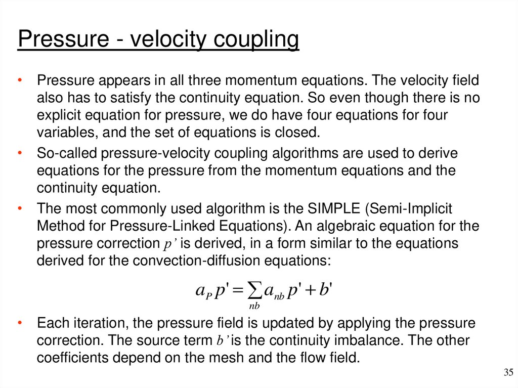
Pressure - velocity coupling• Pressure appears in all three momentum equations. The velocity field
also has to satisfy the continuity equation. So even though there is no
explicit equation for pressure, we do have four equations for four
variables, and the set of equations is closed.
• So-called pressure-velocity coupling algorithms are used to derive
equations for the pressure from the momentum equations and the
continuity equation.
• The most commonly used algorithm is the SIMPLE (Semi-Implicit
Method for Pressure-Linked Equations). An algebraic equation for the
pressure correction p’ is derived, in a form similar to the equations
derived for the convection-diffusion equations:
aP p' anb p' b'
nb
• Each iteration, the pressure field is updated by applying the pressure
correction. The source term b’ is the continuity imbalance. The other
coefficients depend on the mesh and the flow field.
35
32. Properties of numerical schemes
Principle behind SIMPLE• The principle behind SIMPLE is quite simple!
• It is based on the premise that fluid flows from regions with high
pressure to low pressure.
– Start with an initial pressure field.
– Look at a cell.
– If continuity is not satisfied because there is more mass flowing into
that cell than out of the cell, the pressure in that cell compared to the
neighboring cells must be too low.
– Thus the pressure in that cell must be increased relative to the
neighboring cells.
– The reverse is true for cells where more mass flows out than in.
– Repeat this process iteratively for all cells.
• The trick is in finding a good equation for the pressure correction
as a function of mass imbalance. These equations will not be
discussed here but can be readily found in the literature.
36
33. Solution accuracy
Improvements on SIMPLE• SIMPLE is the default algorithm in most commercial finite volume
codes.
• Improved versions are:
– SIMPLER (SIMPLE Revised).
– SIMPLEC (SIMPLE Consistent).
– PISO (Pressure Implicit with Splitting of Operators).
• All these algorithms can speed up convergence because they
allow for the use of larger underrelaxation factors than SIMPLE.
• All of these will eventually converge to the same solution. The
differences are in speed and stability.
• Which algorithm is fastest depends on the flow and there is no
single algorithm that is always faster than the other ones.
37
34. Pressure
Finite volume solution methods• The finite volume solution method can either use a “segregated”
or a “coupled” solution procedure.
• With segregated methods an equation for a certain variable is
solved for all cells, then the equation for the next variable is
solved for all cells, etc.
• With coupled methods, for a given cell equations for all variables
are solved, and that process is then repeated for all cells.
• The segregated solution method is the default method in most
commercial finite volume codes. It is best suited for
incompressible flows or compressible flows at low Mach number.
• Compressible flows at high Mach number, especially when they
involve shock waves, are best solved with the coupled solver.
38
35. Pressure - velocity coupling
Segregated solution procedureUpdate properties.
Solve momentum equations (u, v, w velocity).
Solve pressure-correction (continuity) equation. Update
pressure, face mass flow rate.
Solve energy, species, turbulence, and other scalar equations.
Converged?
No
Yes
Stop
39
36. Principle behind SIMPLE
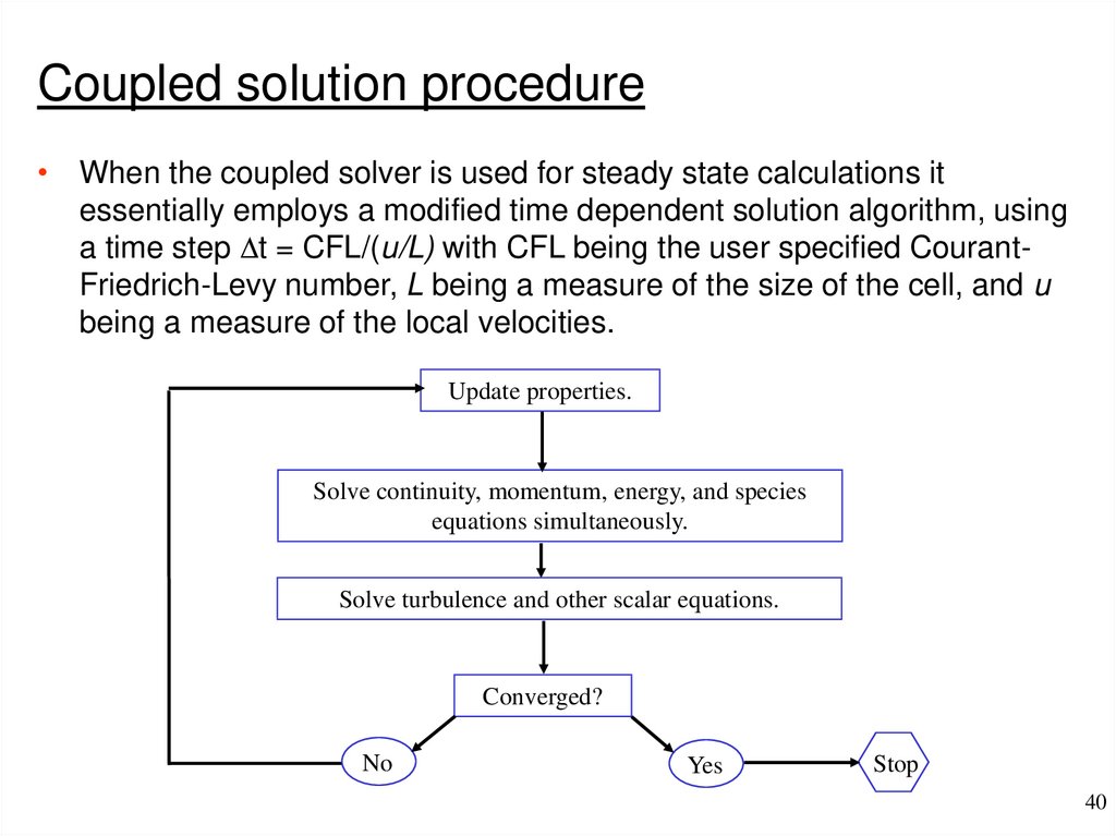
Coupled solution procedure• When the coupled solver is used for steady state calculations it
essentially employs a modified time dependent solution algorithm, using
a time step Dt = CFL/(u/L) with CFL being the user specified CourantFriedrich-Levy number, L being a measure of the size of the cell, and u
being a measure of the local velocities.
Update properties.
Solve continuity, momentum, energy, and species
equations simultaneously.
Solve turbulence and other scalar equations.
Converged?
No
Yes
Stop
40
37. Improvements on SIMPLE
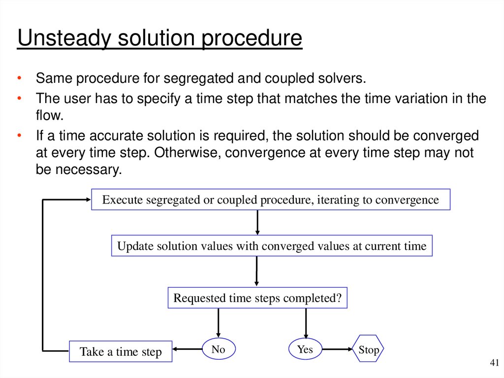
Unsteady solution procedure• Same procedure for segregated and coupled solvers.
• The user has to specify a time step that matches the time variation in the
flow.
• If a time accurate solution is required, the solution should be converged
at every time step. Otherwise, convergence at every time step may not
be necessary.
Execute segregated or coupled procedure, iterating to convergence
Update solution values with converged values at current time
Requested time steps completed?
Take a time step
No
Yes
Stop
41
38. Finite volume solution methods
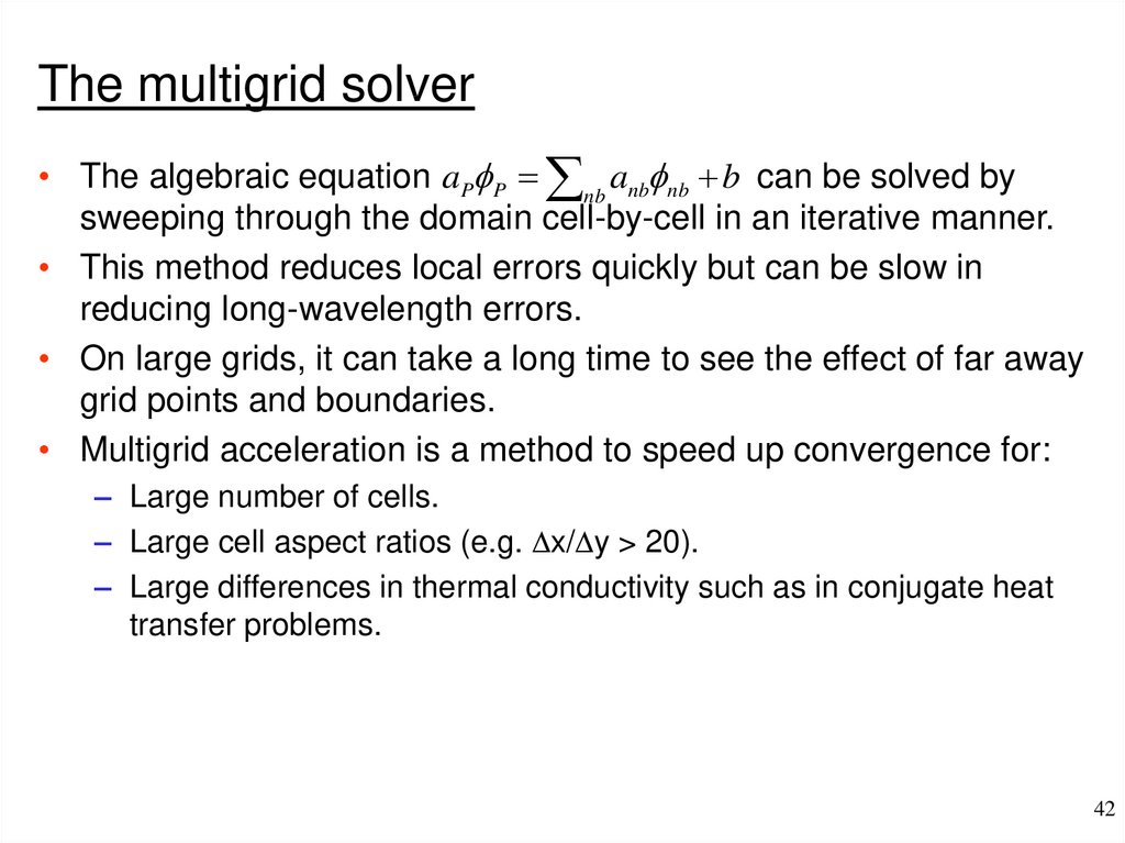
The multigrid solver• The algebraic equation aPf P nb anbfnb b can be solved by
sweeping through the domain cell-by-cell in an iterative manner.
• This method reduces local errors quickly but can be slow in
reducing long-wavelength errors.
• On large grids, it can take a long time to see the effect of far away
grid points and boundaries.
• Multigrid acceleration is a method to speed up convergence for:
– Large number of cells.
– Large cell aspect ratios (e.g. Dx/Dy > 20).
– Large differences in thermal conductivity such as in conjugate heat
transfer problems.
42
39. Segregated solution procedure
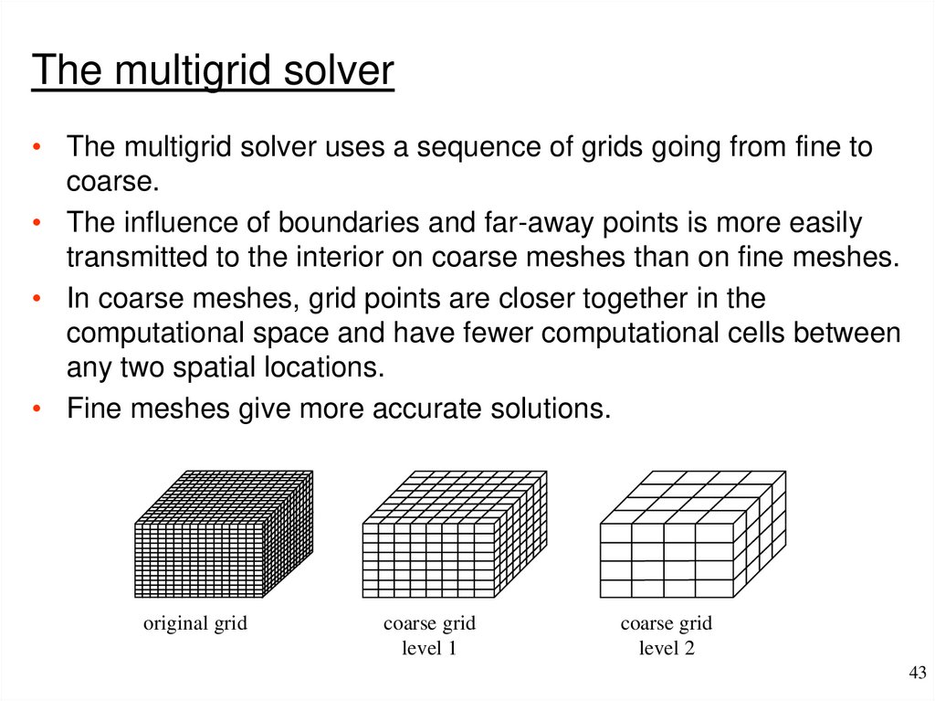
The multigrid solver• The multigrid solver uses a sequence of grids going from fine to
coarse.
• The influence of boundaries and far-away points is more easily
transmitted to the interior on coarse meshes than on fine meshes.
• In coarse meshes, grid points are closer together in the
computational space and have fewer computational cells between
any two spatial locations.
• Fine meshes give more accurate solutions.
original grid
coarse grid
level 1
coarse grid
level 2
43
40. Coupled solution procedure
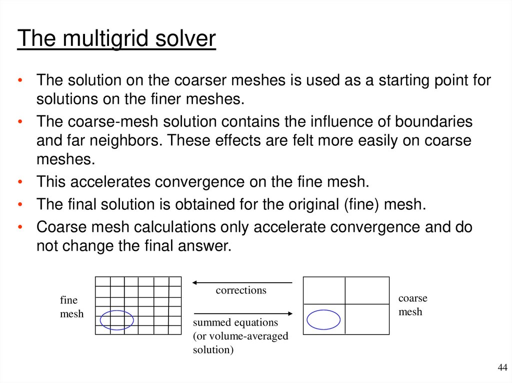
The multigrid solver• The solution on the coarser meshes is used as a starting point for
solutions on the finer meshes.
• The coarse-mesh solution contains the influence of boundaries
and far neighbors. These effects are felt more easily on coarse
meshes.
• This accelerates convergence on the fine mesh.
• The final solution is obtained for the original (fine) mesh.
• Coarse mesh calculations only accelerate convergence and do
not change the final answer.
fine
mesh
corrections
coarse
mesh
summed equations
(or volume-averaged
solution)
44
41. Unsteady solution procedure
Finite volume method - summary• The FVM uses the integral conservation equation applied to
control volumes which subdivide the solution domain, and to the
entire solution domain.
• The variable values at the faces of the control volume are
determined by interpolation. False diffusion can arise depending
on the choice of interpolation scheme.
• The grid must be refined to reduce “smearing” of the solution as
shown in the last example.
• Advantages of FVM: integral conservation is exactly satisfied and
the method is not limited to grid type (structured or unstructured,
Cartesian or body-fitted).
• Always ensure proper convergence.
45







 mathematics


