1D PIC code for TwoStream Plasma Instability

1.

Example: 1D PIC code for TwoStream Plasma Instability

2.

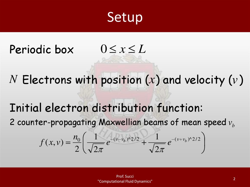
Setup
Periodic box
0 x L
N Electrons with position (x ) and velocity (v )
Initial electron distribution function:
2 counter-propagating Maxwellian beams of mean speed vb
n0 1 ( v vb )^ 2 / 2
1 ( v vb )^ 2 / 2
f ( x, v )
e
e
2 2
2
Prof. Succi
"Computational Fluid Dynamics"
2

3.

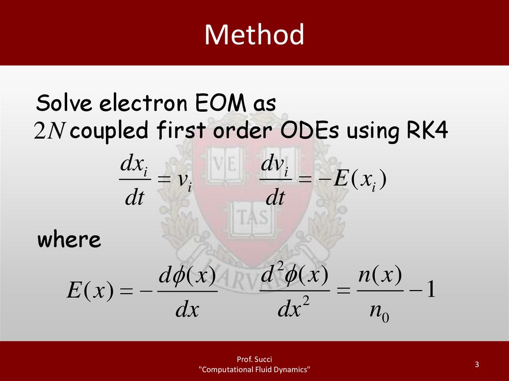
Method
Solve electron EOM as
2 N coupled first order ODEs using RK4
dxi
vi
dt
dvi
E ( xi )
dt
where
d ( x )
E ( x)
dx
d ( x ) n( x )
1
2
dx
n0
2
Prof. Succi
"Computational Fluid Dynamics"
3

4.

Method
Need electric field E (x ) at every time
step. Solve Poisson’s equation (using
spectral method)
Calculate the electron number density n(x )
source term using PIC approach
Prof. Succi
"Computational Fluid Dynamics"
4

5.

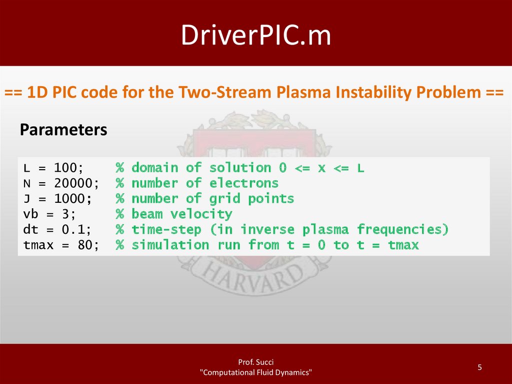
DriverPIC.m
== 1D PIC code for the Two-Stream Plasma Instability Problem ==
Parameters
L = 100;
N = 20000;
J = 1000;
vb = 3;
dt = 0.1;
tmax = 80;
%
%
%
%
%
%
domain of solution 0 <= x <= L
number of electrons
number of grid points
beam velocity
time-step (in inverse plasma frequencies)
simulation run from t = 0 to t = tmax
Prof. Succi
"Computational Fluid Dynamics"
5

6.

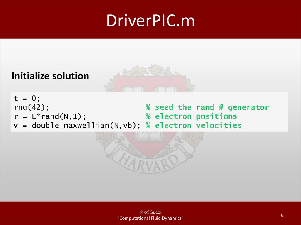
DriverPIC.m
Initialize solution
t = 0;
rng(42);
% seed the rand # generator
r = L*rand(N,1);
% electron positions
v = double_maxwellian(N,vb); % electron velocities
Prof. Succi
"Computational Fluid Dynamics"
6

7.

DriverPIC.m
Evolve solution
while (t<=tmax)
% load r,v into a single vector
solution_coeffs = [r; v];
% take a 4th order Runge-Kutta timestep
k1 = AssembleRHS(solution_coeffs,L,J);
k2 = AssembleRHS(solution_coeffs + 0.5*dt*k1,L,J);
k3 = AssembleRHS(solution_coeffs + 0.5*dt*k2,L,J);
k4 = AssembleRHS(solution_coeffs + dt*k3,L,J);
solution_coeffs = solution_coeffs + dt/6*(k1+2*k2+2*k3+k4);
% unload solution coefficients
r = solution_coeffs(1:N);
v = solution_coeffs(N+1:2*N);
% make sure all coordinates are in the range 0 to L
r = r + L*(r<0) - L*(r>L);
t = t + dt;
end
Prof. Succi
"Computational Fluid Dynamics"
7

8.

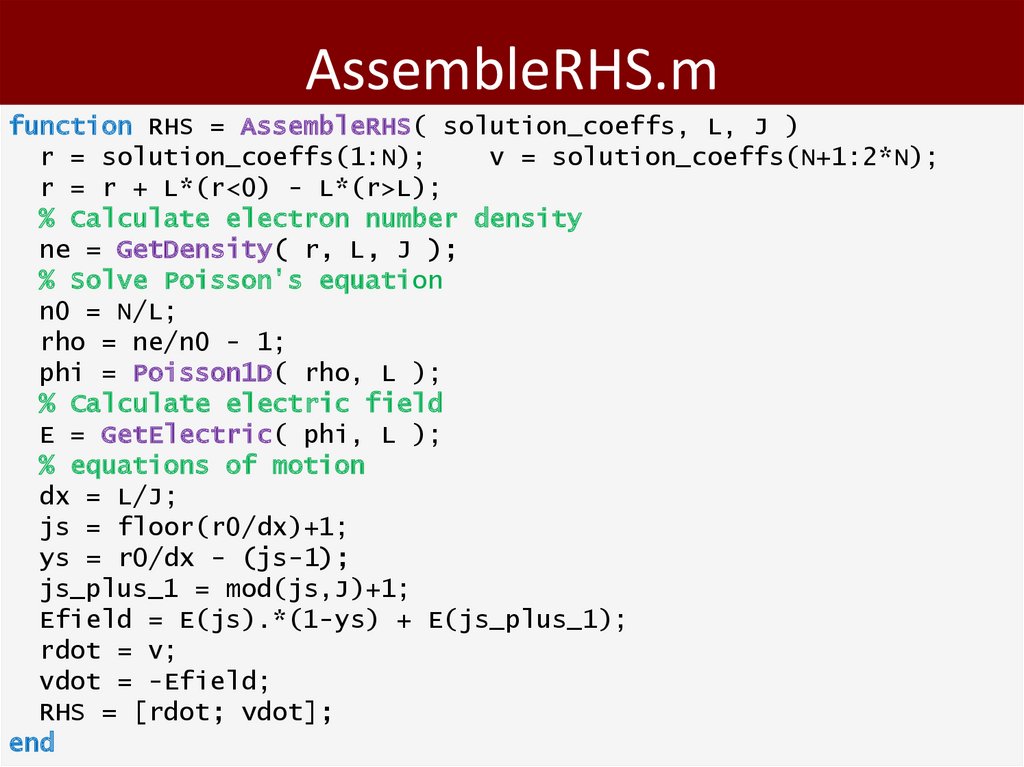
AssembleRHS.m
function RHS = AssembleRHS( solution_coeffs, L, J )
r = solution_coeffs(1:N);
v = solution_coeffs(N+1:2*N);
r = r + L*(r<0) - L*(r>L);
% Calculate electron number density
ne = GetDensity( r, L, J );
% Solve Poisson's equation
n0 = N/L;
rho = ne/n0 - 1;
phi = Poisson1D( rho, L );
% Calculate electric field
E = GetElectric( phi, L );
% equations of motion
dx = L/J;
js = floor(r0/dx)+1;
ys = r0/dx - (js-1);
js_plus_1 = mod(js,J)+1;
Efield = E(js).*(1-ys) + E(js_plus_1);
rdot = v;
vdot = -Efield;
RHS = [rdot; vdot];
Prof. Succi
"Computational Fluid Dynamics"
end
8

9.

GetDensity.m
function n = GetDensity( r, L, J )
% Evaluate number density n in grid of J cells, length
L, from the electron positions r
dx = L/J;
js = floor(r/dx)+1;
ys = r/dx - (js-1);
js_plus_1 = mod(js,J)+1;
n = accumarray(js,(1-ys)/dx,[J,1]) + ...
accumarray(js_plus_1,ys/dx,[J,1]);
end
Prof. Succi
"Computational Fluid Dynamics"
9

10.

Poisson1D.m
function u = Poisson1D( v, L )
% Solve 1-d Poisson equation:
%
d^u / dx^2 = v
for 0 <= x <= L
% using spectral method
J = length(v);
% Fourier transform source term
v_tilde = fft(v);
% vector of wave numbers
k = (2*pi/L)*[0:(J/2-1) (-J/2):(-1)]';
k(1) = 1;
% Calculate Fourier transform of u
u_tilde = -v_tilde./k.^2;
% Inverse Fourier transform to obtain u
u = real(ifft(u_tilde));
% Specify arbitrary constant by forcing corner u = 0;
u = u - u(1);
end
Prof. Succi
"Computational Fluid Dynamics"
10

11.

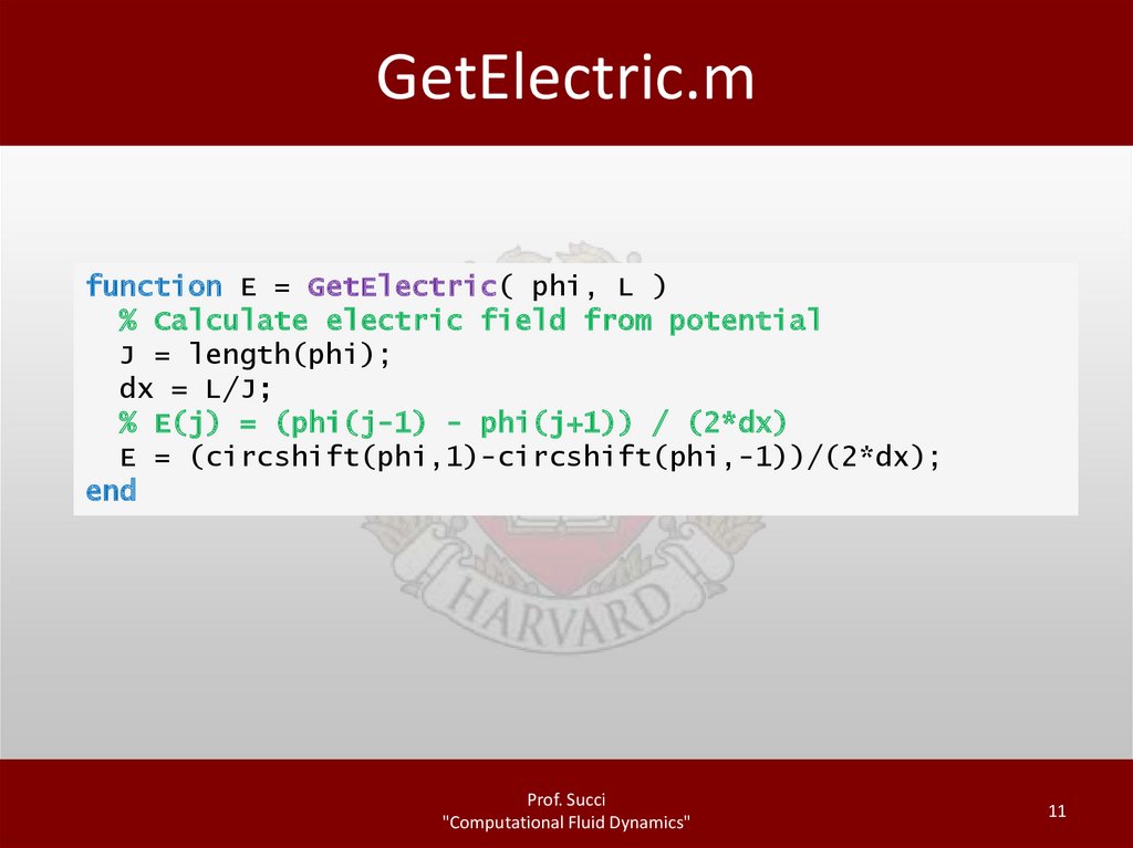
GetElectric.m
function E = GetElectric( phi, L )
% Calculate electric field from potential
J = length(phi);
dx = L/J;
% E(j) = (phi(j-1) - phi(j+1)) / (2*dx)
E = (circshift(phi,1)-circshift(phi,-1))/(2*dx);
end
Prof. Succi
"Computational Fluid Dynamics"
11

12.

Results
Prof. Succi
"Computational Fluid Dynamics"
12