Chapter 25. Capturing Equity Risk Premia

1. Chapter 25

Capturing Equity Risk
Premia*
By
Cheng Few Lee
Joseph Finnerty
John Lee
Alice C Lee
Donald Wort
* This chapter was written by Jose Menchero (MSCI
barra), Andrei Morozov (MSCI Inc.) and John Guerard
(McKinley Capital Management).

2. Outline

• 25.1
GLOBAL EQUITY RISK MODEL
25.1.1 Estimation Universe
25.1.2 GEM2 Factor Structure
• 25.2 FACTOR PORTFOLIOS
25.2.1 Simple Factor Portfolios
25.2.2 Pure Factor Portfolios
25.2.3 Optimized Factor Portfolios
• 25.3 RESULTS
25.3.1 Cumulative Factor Returns
25.3.2 Summary Statistics
• 25.4 LEADING ECONOMIC INDICATORS AND
BARRA FACTOR RETURNS
• 25.5 SUMMARY
2

3. 25.1 GLOBAL EQUITY RISK MODEL 25.1.1 Estimation Universe

25.1 GLOBAL EQUITY RISK
MODEL
•25.1.1
Estimation
The estimation
universe
Universe
is
the set of stocks that is used to estimate the model. Judicious
selection of the estimation universe is a critical component to building a sound risk model.
The estimation universe must be sufficiently broad to accurately represent the investment
opportunity set of global investors, without being so broad as to include illiquid stocks that
may introduce spurious return relationships into the model. Furthermore, the estimation
universe should be reasonably stable to ensure that factor exposures are well behaved
across time. Representation, liquidity, and stability, therefore, represent the three primary
goals that must be attained when selecting a risk model estimation universe.
3
A well-constructed equity index must address and overcome these very issues, and
therefore serves as an excellent foundation for the estimation universe. The GEM2
estimation universe utilizes the MSCI All Country World Investable Market Index (ACWI
IMI), part of the MSCI Global Investable Market Indices family, which represents the
latest in MSCI index-construction methodology. MSCI ACWI IMI aims to reflect the full
breadth of global investment opportunities by targeting 99% of the float-adjusted market
capitalization in both developed and emerging markets. The index-construction
methodology applies innovative rules designed to achieve index stability, while reflecting
the evolving equity markets in a timely fashion. Moreover, liquidity screening rules are
applied to ensure that only investable stocks with reliable pricing are included for index
membership.

4. 25.1 GLOBAL EQUITY RISK MODEL 25.1.2 GEM2 Factor Structure

• The
equity factor set in GEM2 includes a World factor (w) ,
countries (c) , industries (i) , and styles (s). Every stock is assigned
an exposure of 1 to the World factor. Hence, the local excess returns
(i.e., currency hedged) can be written as
rn f w X n c f c X n i f i • X n s f s un
c
• where
i
s
(25.1)
Xnk is the exposure of stock n to factor k, fk is the return of the
factor, and Un is the specific return of the stock. Mathematically,
the World factor represents the intercept term in the cross-sectional
regression. Economically, it describes the aggregate up-and-down
movement of the global equity market. Typically, the World factor
is the dominant source of risk for a diversified long-only portfolio.
4

5. 25.1 GLOBAL EQUITY RISK MODEL 25.1.2 GEM2 Factor Structure

5
Table 25-1 GEM2 Country Factors
Average weights (based on total capitalization) are
from January 1997 to January 2008. Market
capitalizations are reported in trillions of US
dollars.

6. 25.1 GLOBAL EQUITY RISK MODEL 25.1.2 GEM2 Factor Structure

Table 25-2 GEM2 Industry
Factors
6
Weights are computed within the
GEM2 estimation universe using
total market capitalization. Average
weights are computed from January
1997 to January 2008.

7. 25.1 GLOBAL EQUITY RISK MODEL 25.1.2 GEM2 Factor Structure

Unlike country and industry factors, which are assigned exposures of either
0 or 1, style factor exposures are continuously distributed. To facilitate
comparison across style factors, they are standardized to have a mean of 0
and a standard deviation of 1. Each descriptor is also standardized similarly.
Raw
That is, if d nl is the raw value of stock n for descriptor l,
then the standardized descriptor value is given by
• (25.2)
d nlRaw l
d nl
7
l
where μl is the cap-weighted mean of the descriptor (within the estimation
universe), and σl is the equal-weighted standard deviation. the convention of
standardizing using the cap-weighted mean so that a well-diversified capweighted global portfolio, such as MSCI ACWI IMI, has approximately zero
exposure to all style factors is adopted. For the standard deviation, however,
the equal-weighted mean to prevent large-cap stocks from having an undue
influence on the overall scale of the exposures is used.

8. 25.1 GLOBAL EQUITY RISK MODEL 25.1.2 GEM2 Factor Structure

25.1 GLOBAL EQUITY RISK
MODEL
GEM2
Factor
•25.1.2
Formally,
descriptors
areStructure
combined into
style factors as follows:
X nk wl d nl
(25.3)
l k
8
where wl is the descriptor weight, and the sum takes place over all
descriptors within a particular risk index. Descriptor weights are determined
using an optimization algorithm to maximize the explanatory power of the
model. Style factor exposures are rescaled to have a standard deviation of 1.
Some of the style factors are standardized on a global-relative basis, others
on a country-relative basis. In the former case, the mean and standard
deviation in Equation 25.2 are computed using the entire global cross
section. In the latter case, the factors have mean 0 and standard deviation 1
within each country. When deciding which standardization convention to
adopt, both the intuitive meaning of the factor and its explanatory power are
considered.

9. 25.1 GLOBAL EQUITY RISK MODEL 25.1.2 GEM2 Factor Structure

Table 25-3 RegressionWeighted Cross-sectional
Correlation of Style and
Industry Factor Exposures
9
Results are averages over the
period from January 1997 to June
2008. Correlations above 0.10 in
absolute value are shaded in gray.

10. 25.1 GLOBAL EQUITY RISK MODEL 25.1.2 GEM2 Factor Structure

GEM2 uses eight style factors. Specific details on the individual descriptors
comprising each style factor can be found in Menchero et al. (2010). Below, a
qualitative description of each of the style factors are provided:
10
(1) The Volatility factor is typically the most significant style factor. In essence, it
captures market risk that cannot be explained by the World factor. The most
important descriptor within the Volatility index is historical beta relative to the
World portfolio (as proxied by the estimation universe). To better understand this
factor, consider a fully invested long-only portfolio that is strongly tilted toward
high-beta stocks. Intuitively, this portfolio has greater market risk than a portfolio
with beta equal to one. This additional market risk is captured through positive
exposure to the Volatility factor. Note that the time-series correlation between the
World factor and the Volatility factor is typically very high, so that these two
sources of risk add coherently in this example. If, by contrast, the portfolio is
invested in low-beta stocks, then the risk from the Volatility and the World factors
is partially canceled, as intuitively expected. The Volatility factor on a globalrelative basis is standardized. As a result, the mean exposure to Volatility within a
country can deviate significantly from zero. This standardization convention is a
natural one for a global model, as most investors regard stocks in highly volatile
markets as having more exposure to the factor than those in low-volatility markets.
This view is reflected in the data, as it is found that the explanatory power of the

11. 25.1 GLOBAL EQUITY RISK MODEL 25.1.2 GEM2 Factor Structure

(2) The Momentum factor often ranks second in significance after Volatility.
Momentum differentiates stocks based on recent relative performance. Descriptors
within Momentum include historical alpha from a 104-week regression and relative
strength (over trailing 6 and 12 months) with a one-month lag. As with Volatility,
Momentum is standardized on a global-relative basis. This is also an intuitive
convention for a global model. From the perspective of a global investor, a stock
that strongly outperforms the World portfolio is likely to be considered a positive
momentum stock, even if it slightly underperforms its country peers. The empirical
results support this view, as the Momentum factor standardized globally has greater
explanatory power than one standardized on a country-relative basis.
11
(3) The Size factor represents another well-known source of return covariance. It
captures the effect of large-cap stocks moving differently from small-cap stocks.
Size is measured by a single descriptor: log of market capitalization. The
explanatory power of the model is quite similar whether Size is standardized
globally or on a country-by-country basis. The country-relative standardization is
adopted, however, since it is more intuitive and consistent with investors’
perception of the markets. For instance, major global equity indices, such as the
MSCI Global Investable Market Indices, segment each country according to size,
with the largest stocks inside each country always being classified as large-cap
stocks. Moreover, standardizing the Size factor on a global-relative basis would

12. 25.1 GLOBAL EQUITY RISK MODEL 25.1.2 GEM2 Factor Structure

(4) The Value factor describes a major investment style which seeks to identify stocks
that are priced low relative to fundamentals. Value is standardized on a countryrelative basis. This again is consistent with the way major indices segment each
market, with each country divided roughly equally into value and growth
subindices. This convention also circumvents the difficulty of comparing
fundamental data across countries with different accounting standards. GEM2
utilizes official MSCI data items for Value factor descriptors, as described in the
MSCI Barra Fundamental Data Methodology handbook (2008).
(5) Growth differentiates stocks based on their prospects for sales or earnings growth.
It is standardized on a country-relative basis, consistent with the construction of the
MSCI Value and Growth Indices. Therefore, each country has approximately half
the weight in stocks with positive Growth exposure, and half with negative
exposure. The GEM2 Growth descriptors also utilize official MSCI data items, as
described in the MSCI Barra Fundamental Data Methodology handbook.
12

13. 25.1.2 GEM2 Factor Structure

(6) The Nonlinear Size (NLS) factor captures nonlinearities in the payoff to
size exposure across the market-cap spectrum. NLS is based on a single raw
descriptor: the cube of the log of market capitalization. Since this raw
descriptor is highly collinear with Size, it is orthogonalized to the Size
factor. This procedure does not affect the fit of the model, but does mitigate
the confounding effects of collinearity, and thus preserves an intuitive
meaning for the Size factor. The NLS factor is represented by a portfolio that
goes long mid-cap stocks, and shorts large-cap and small-cap stocks.
(7) The Liquidity factor describes return patterns to stocks based on relative
trading activity. Stocks with high turnover have positive exposure to
Liquidity, whereas low-turnover stocks have negative exposure. Liquidity is
standardized on a country-relative basis.
(8) Leverage captures the return difference between high-leverage and lowleverage stocks. The descriptors within Leverage include market leverage,
book leverage, and debt-to-assets ratio. This factor is standardized on a
country-relative basis.
13

14. 25.2 FACTOR PORTFOLIOS 25.2.1 Simple Factor Portfolios

Simple factor portfolios are formed from a univariate regression of local
excess returns,
s
s
s
(25.4)
rn f w X ns f s un
14
where the intercept term
sis the return to the simple World factor,
f w style factor, and s is the residual. The
s is the return to the simple
fs
GEM2
model uses square root of market cap foruthe
n regression weights.
This is appropriate for risk model construction since to a good
approximation it minimizes sampling error. In this chapter, however, the
objective is to study the performance of long/short investment strategies.
For this purpose, it is more appropriate to focus on large-cap stocks which
are more easily shorted than relatively illiquid small-cap stocks. Therefore,
market-cap weights wn is used in the regression.

15. 25.2 FACTOR PORTFOLIOS 25.2.1 Simple Factor Portfolios

• As
discussed by Menchero (2010), with style factor exposures standardized to
be cap-weighted mean 0 and standard deviation 1, the World factor return is
given by
f ws wn rn
n
(25.5)
• which
is simply the cap-weighted return (currency hedged) of the World
portfolio. The simple style factor returns are given by
f ss ( wn X• ns ) rn
n
• which
(25.6)
represents the return of a factor-replicating portfolio that goes long stocks
with positive exposure to the factor, and shorts stocks with negative exposure.
The weights are also proportional to the market cap, so that the portfolio is
dominated by large-cap stocks.
15

16. 25.2 FACTOR PORTFOLIOS 25.2.2 Pure Factor Portfolios

f kp
• Pure
factor returns
are estimated by cross-sectional regression of local excess
returns against all the factors,
rn X nk f k p unp
k
(25.7)
• The
index k runs over the World factor, countries, industries, and styles. Again,
although the GEM2 risk model uses square root of market cap for the regression
weights, in this study market cap weights for the regression is employed.
Every stock has unit exposure to the World factor, and exposure of 0 or 1 to
countries and industries. As a result, the sum of all country factor exposures Xnc
equals the World factor exposure, and similarly for industries, i.e.,
X
c
• for
nc
1,
and
X
i
ni
1
(25.8)
all stocks . The GEM2 factor structure, therefore, exhibits exact two-fold
collinearity. Constraints must be applied to obtain a unique solution.
16

17. 25.2 FACTOR PORTFOLIOS 25.2.2 Pure Factor Portfolios

• We
adopt constraints as in Heston and Rouwenhorst (1994) that require the cap-weighted
country and industry factor returns to sum to zero,
p
W
f
c c 0,
and
c
p
W
f
i i 0
(25.9)
i
• where
Wc is the cap weight of the estimation universe in country c and Wi is the
corresponding weight in industry i. These constraints remove the exact collinearities from
the factor exposure matrix, without reducing the explanatory power of the model.
• A more precise interpretation to the factors can be provided now. Consider the cap-weighted
world portfolio, with asset weights wn. The currency-hedged return of this portfolio Rw can
be attributed using the GEM2 factors,
p
w p
p
Rw f wp Wc f c p
• Wi f i X s f s wn u n
c
• The
i
s
(25.10)
n
first two sums in Equation (25.10) are equal to zero by virtue of the constraints of
Equation (25.9). The third sum is zero since the style factors are standardized
to be capw
0 s.
weighted mean zero for the world portfolio; i.e.,
, forXall
styles
s
17

18. 25.2 FACTOR PORTFOLIOS 25.2.2 Pure Factor Portfolios

• The
final sum in Equation (25.10) is the cap-weighted specific return of the estimation
universe, which is equal to zero by virtue of using cap-weights in the regression. Therefore,
Rw f
p
w
(25.11)
• which
means that the return of the pure World factor is exactly the cap-weighted return of the
world portfolio. That is, for this regression setting, the simple and pure World factors are
identical.
• The pure style factor returns can be written as
f s p •W nsp rn
W
n
(25.12)
p
• Where
is the weight of stock n in pure factor portfolio s. The pure factor
ns
portfolio has unit exposure to the particular style, but zero exposure to all other factors. This
implies, for example, that the pure style factor portfolio has net zero weight in every industry
and every country. For a more extensive discussion of pure factor portfolios, see Menchero
(2010).
18

19. 25.2 FACTOR PORTFOLIOS 25.2.3 Optimized Factor Portfolios

• Simple
factor portfolios have unit exposure to the particular factor, and
nonzero exposure to other factors. Pure factor portfolios have unit
exposure to the particular factor, and zero exposure to all other factors.
There is another important factor portfolio to consider. This is given
by the minimum risk portfolio with unit exposure to the factor.
• The solution, as shown by Grinold and Kahn (2000), is given by
æ
öæ
ö
Wons ç Vmn 1 X ms ÷ç X nsVmn• 1 X ms ÷
è m
øè mn
ø
• where
Vmn 1
1
(25.13)
is the element (between stocks m and n) of the inverse asset
covariance matrix. The intuition behind optimized factor portfolios is
straightforward: the portfolio maintains unit exposure to the particular
factor but reduces the risk by acquiring exposures to other factors.
19

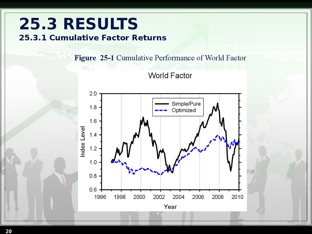
20. 25.3 RESULTS 25.3.1 Cumulative Factor Returns

Figure 25-1 Cumulative Performance of World Factor
World Factor
2.0
Simple/Pure
Optimized
1.8
Index Level
1.6
1.4
1.2
1.0
0.8
0.6
1996
1998
2000
2002
2004
Year
20
2006
2008
2010

21. 25.3 RESULTS 25.3.1 Cumulative Factor Returns

Figure 25-2 Cumulative Performance of Value Factor
Value Factor
2.0
1.8
Index Level
1.6
1.4
1.2
1.0
Simple
Pure
Optimized
0.8
0.6
1996
1998
2000
2002
2004
Year
21
2006
2008
2010

22. 25.3 RESULTS 25.3.1 Cumulative Factor Returns

Figure 25-3 Cumulative Performance of Momentum Factor
Momentum Factor
2.4
Simple
Pure
Optimized
2.2
Index Level
2.0
1.8
1.6
1.4
1.2
1.0
0.8
1996
1998
2000
2002
2004
Year
22
2006
2008
2010

23. 25.3 RESULTS 25.3.1 Cumulative Factor Returns

Figure 25-4 Cumulative Performance of Size Factor
Size Factor
1.3
Simple
Pure
Optimized
Index Level
1.2
1.1
1.0
0.9
0.8
0.7
1996
1998
2000
2002
2004
Year
23
2006
2008
2010

24. 25.3 RESULTS 25.3.1 Cumulative Factor Returns

Figure 25-5 Cumulative Performance of Volatility Factor
Volatility Factor
1.5
1.4
Simple
Pure
Optimized
Index Level
1.3
1.2
1.1
1.0
0.9
0.8
0.7
0.6
1996
1998
2000
2002
2004
Year
24
2006
2008
2010

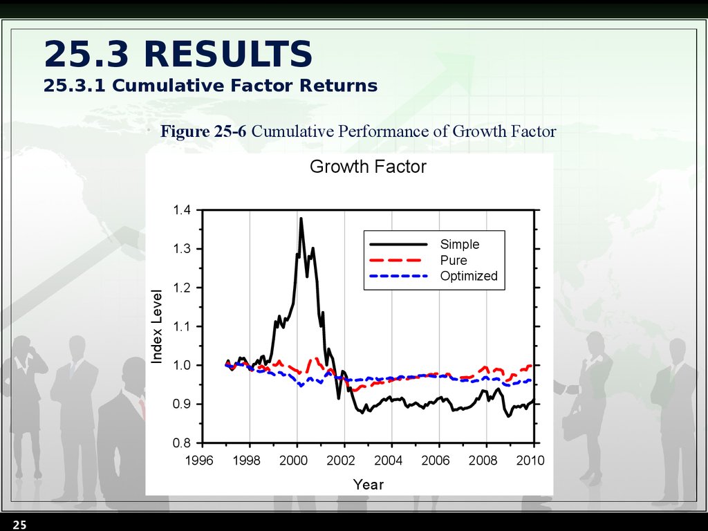
25. 25.3 RESULTS 25.3.1 Cumulative Factor Returns

Figure 25-6 Cumulative Performance of Growth Factor
Growth Factor
1.4
Simple
Pure
Optimized
Index Level
1.3
1.2
1.1
1.0
0.9
0.8
1996
1998
2000
2002
2004
Year
25
2006
2008
2010

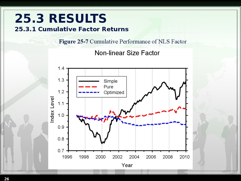
26. 25.3 RESULTS 25.3.1 Cumulative Factor Returns

Figure 25-7 Cumulative Performance of NLS Factor
Non-linear Size Factor
1.4
1.3
Simple
Pure
Optimized
Index Level
1.2
1.1
1.0
0.9
0.8
0.7
1996
1998
2000
2002
2004
Year
26
2006
2008
2010

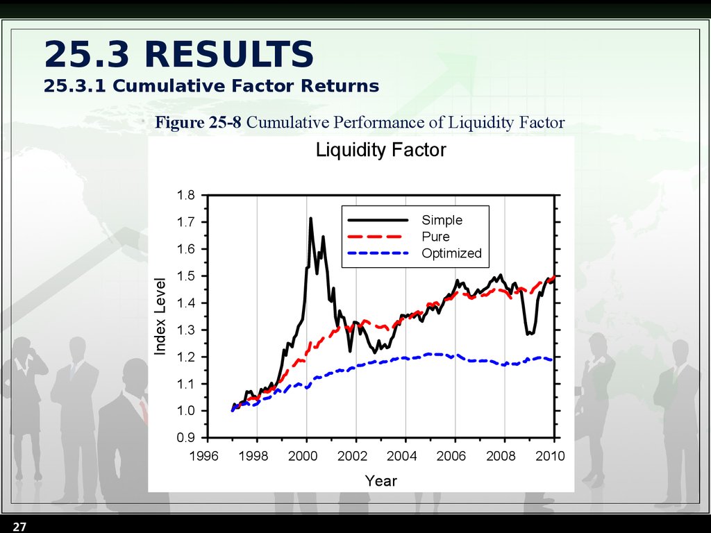
27. 25.3 RESULTS 25.3.1 Cumulative Factor Returns

Figure 25-8 Cumulative Performance of Liquidity Factor
Liquidity Factor
1.8
Simple
Pure
Optimized
1.7
Index Level
1.6
1.5
1.4
1.3
1.2
1.1
1.0
0.9
1996
1998
2000
2002
2004
Year
27
2006
2008
2010

28. 25.3 RESULTS 25.3.1 Cumulative Factor Returns

Figure 25-9 Cumulative Performance of Leverage Factor
Leverage Factor
1.2
Simple
Pure
Optimized
Index Level
1.1
1.0
0.9
0.8
1996
1998
2000
2002
2004
Year
28
2006
2008
2010

29. 25.1 GLOBAL EQUITY RISK MODEL 25.3.2 Summary Statistics

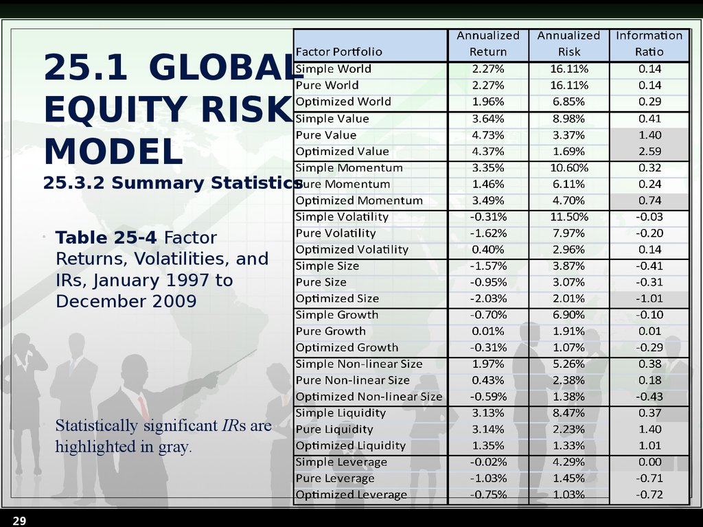
29
Table 25-4 Factor
Returns, Volatilities, and
IRs, January 1997 to
December 2009
Statistically significant IRs are
highlighted in gray.

30. 25.1 GLOBAL EQUITY RISK MODEL 25.3.2 Summary Statistics

30
Table 25-5 Time-Series
Correlations, January
1997 to December 2009

31. 25.4 LEADING ECONOMIC INDICATORS AND BARRA FACTOR RETURNS

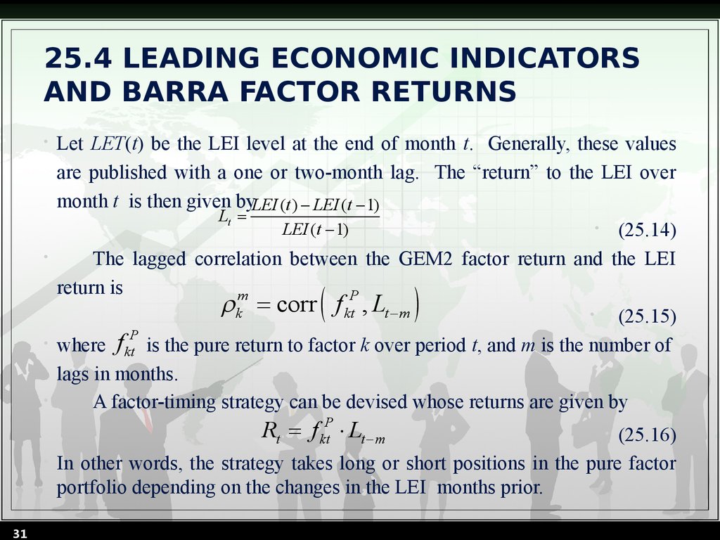
Let LET(t) be the LEI level at the end of month t. Generally, these values
are published with a one or two-month lag. The “return” to the LEI over
month t is then given byLEI (t ) LEI (t 1)
Lt
• (25.14)
LEI (t 1)
The lagged correlation between the GEM2 factor return and the LEI
return is
r km corr f ktP , Lt m
(25.15)
P
where f kt is the pure return to factor k over period t, and m is the number of
lags in months.
A factor-timing strategy can be devised whose returns are given by
(
Rt f ktP × Lt m
31
)
(25.16)
In other words, the strategy takes long or short positions in the pure factor
portfolio depending on the changes in the LEI months prior.

32. 25.4 LEADING ECONOMIC INDICATORS AND BARRA FACTOR RETURNS

32
Table 25-6 Lagged Correlations between Monthly GEM2 Pure Factor
Returns and Monthly Percentage Changes in the European LEI
Levels
Analysis period: January 1997 to December 2009.

33. 25.4 LEADING ECONOMIC INDICATORS AND BARRA FACTOR RETURNS

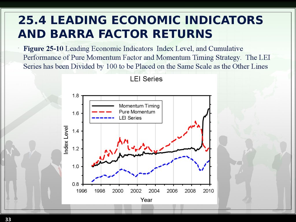
Figure 25-10 Leading Economic Indicators Index Level, and Cumulative
Performance of Pure Momentum Factor and Momentum Timing Strategy. The LEI
Series has been Divided by 100 to be Placed on the Same Scale as the Other Lines
LEI Series
1.8
Momentum Timing
Pure Momentum
LEI Series
Index Level
1.6
1.4
1.2
1.0
0.8
1996
1998
2000
2002
2004
Year
33
2006
2008
2010

34. 25.5 SUMMARY

34
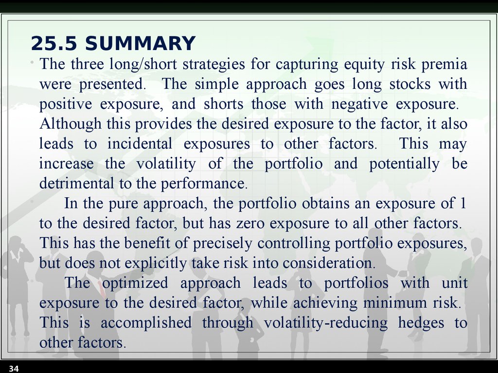
The three long/short strategies for capturing equity risk premia
were presented. The simple approach goes long stocks with
positive exposure, and shorts those with negative exposure.
Although this provides the desired exposure to the factor, it also
leads to incidental exposures to other factors. This may
increase the volatility of the portfolio and potentially be
detrimental to the performance.
In the pure approach, the portfolio obtains an exposure of 1
to the desired factor, but has zero exposure to all other factors.
This has the benefit of precisely controlling portfolio exposures,
but does not explicitly take risk into consideration.
The optimized approach leads to portfolios with unit
exposure to the desired factor, while achieving minimum risk.
This is accomplished through volatility-reducing hedges to
other factors.

35. 25.5 SUMMARY

35
The performance of eight style factors and the World factor over
a 13-year period were examined. None of the simple strategies
achieved a statistically significant IR over this period. For the
pure style factors, three were statistically significant, versus five
for the optimized factors. For Value, Size, and Momentum, the
optimized strategies had far higher IRs than the pure
counterparts.
Finally, an illustrative example of a Momentum “factor
timing” strategy that uses lagged LEI values as the input signal
was considered. It was found that, on a risk-adjusted basis, the
factor timing strategy outperformed the pure Momentum factor
over the sample period.