
 mathematics
Similar presentations:


T PM N 2019/2020 : Solving the Schr¨odingerequation
1.
T PM N 2019/2020 : Solving the Schr¨odingerequatione M. Alouani, mebarek.alouani@ipcms.unistra.fr, IPCMS
e H. Bulou, herve.bulou@ipcms.unistra.fr, IPCMS
2.
T PM N 2019/2020 : Solving the Schr¨odingerequatione M. Alouani, mebarek.alouani@ipcms.unistra.fr, IPCMS
e H. Bulou, herve.bulou@ipcms.unistra.fr, IPCMS
e Aim of this course : Solving the Sch¨odinger equation by using acomputer
HΨ( r ) = sΨ(r )
3.
T PM N 2019/2020 : Solving the Schr¨odingerequatione M. Alouani, mebarek.alouani@ipcms.unistra.fr, IPCMS
e H. Bulou, herve.bulou@ipcms.unistra.fr, IPCMS
e Aim of this course : Solving the Sch¨odinger equation by using a computer
HΨ( r ) = sΨ(r )
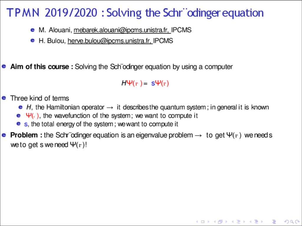
e Three kind of terms
e H, the Hamiltonian operator → it describes the quantum system ; in general it is known
e Ψ(r ), the wavefunction of the system; we want to compute it
e s, the total energy of the system ; we want to compute it
4.
T PM N 2019/2020 : Solving the Schr¨odingerequatione M. Alouani, mebarek.alouani@ipcms.unistra.fr, IPCMS
e H. Bulou, herve.bulou@ipcms.unistra.fr, IPCMS
e Aim of this course : Solving the Sch¨odinger equation by using a computer
HΨ( r ) = sΨ(r )
e Three kind of terms
e H, the Hamiltonian operator → it describes the quantum system ; in general it is known
e Ψ(r ), the wavefunction of the system; we want to compute it
e s, the total energy of the system ; we want to compute it
e Problem : the Schr¨odinger equation is an eigenvalue problem → to get Ψ( r ) we need s
we to get s we need Ψ( r )!
5.
T PM N 2019/2020 : Solving the Schr¨odingerequatione M. Alouani, mebarek.alouani@ipcms.unistra.fr, IPCMS
e H. Bulou, herve.bulou@ipcms.unistra.fr, IPCMS
e Aim of this course : Solving the Sch¨odinger equation by using a computer
HΨ( r ) = sΨ(r )
e Three kind of terms
e H, the Hamiltonian operator → it describes the quantum system ; in general it is known
e Ψ(r ), the wavefunction of the system; we want to compute it
e s, the total energy of the system ; we want to compute it
e Problem : the Schr¨odinger equation is an eigenvalue problem → to get Ψ( r ) we need s
we to get s we need Ψ( r )!
e From a numerical point of view, there are different ways to solve this problem
e Tomorrow, we will see a quite general method : the Finite Difference Method
e Next week, R. Hertel will present another possible way to proceed : the Finite Element
Method
e Today, we’re going to see a method which can be use in very specific cases : the Numerov
Method
6.
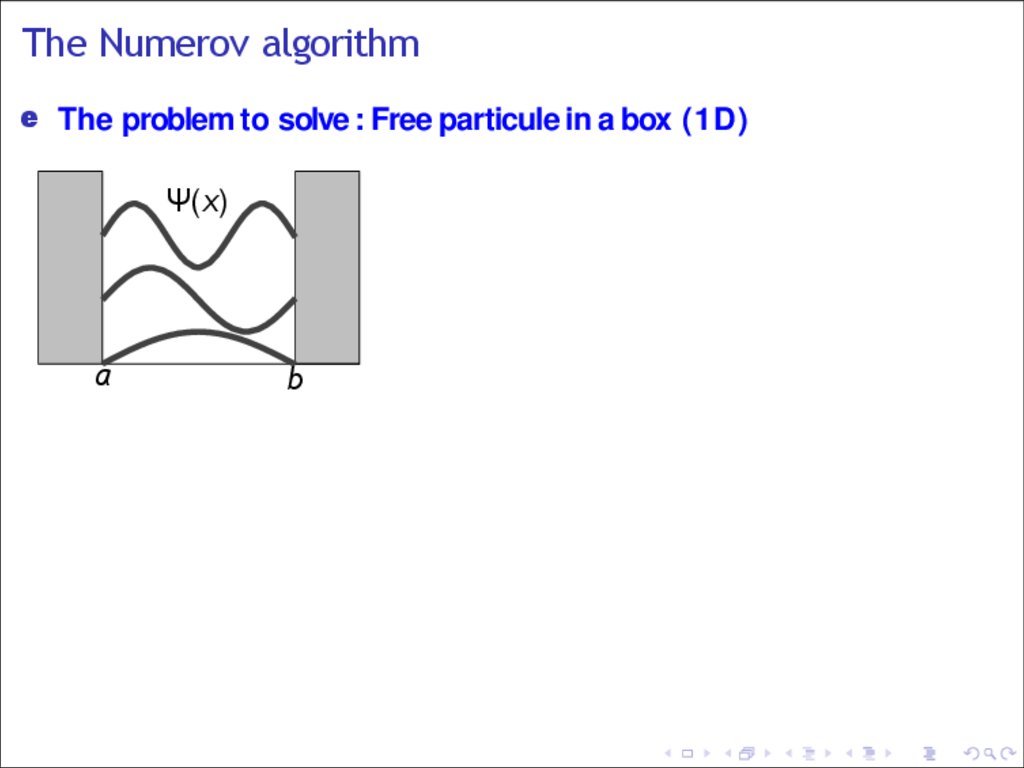
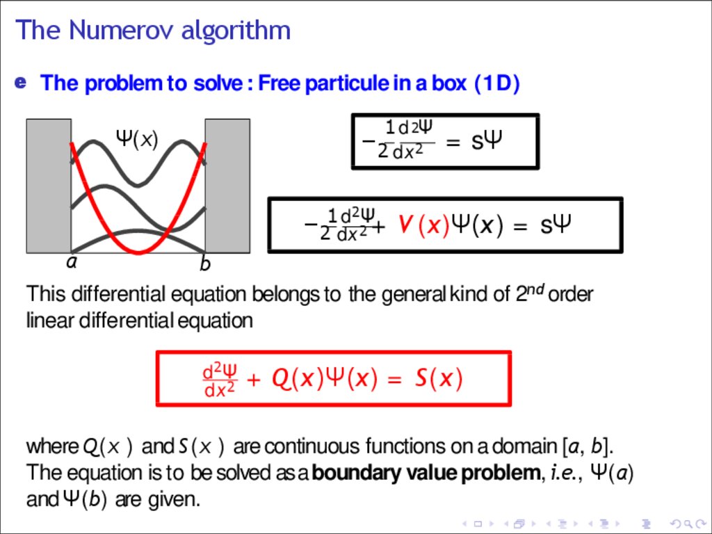
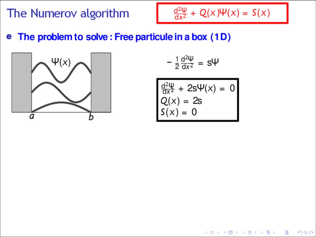
The Numerov algorithme The problem to solve : Free particule in a box (1D)
Ψ(x)
a
b
7.
The Numerov algorithme The problem to solve : Free particule in a box (1D)
1 d 2Ψ
Ψ(x)
a
−2 dx 2 = sΨ
b
8.
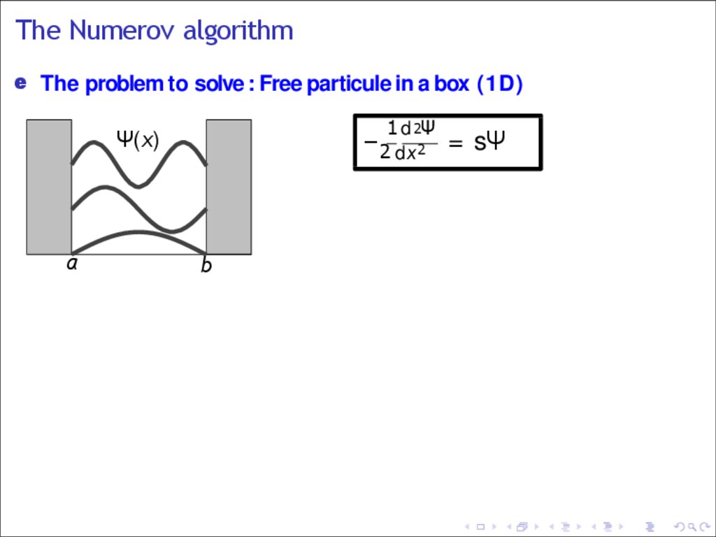
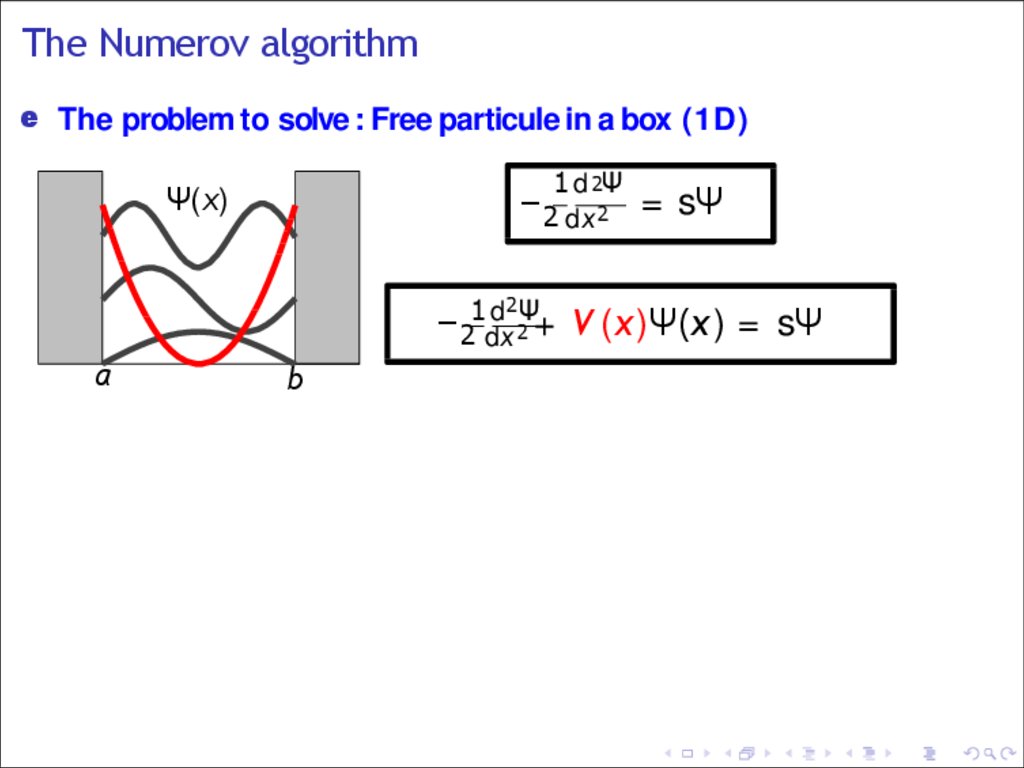
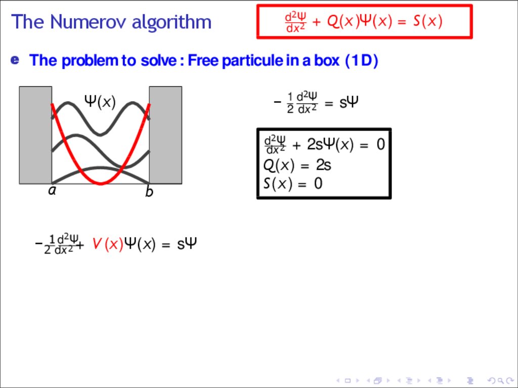
The Numerov algorithme The problem to solve : Free particule in a box (1D)
1 d 2Ψ
Ψ(x)
−2 dx 2 = sΨ
2
d Ψ
−21dx
2 + V (x)Ψ(x ) = sΨ
a
b
9.
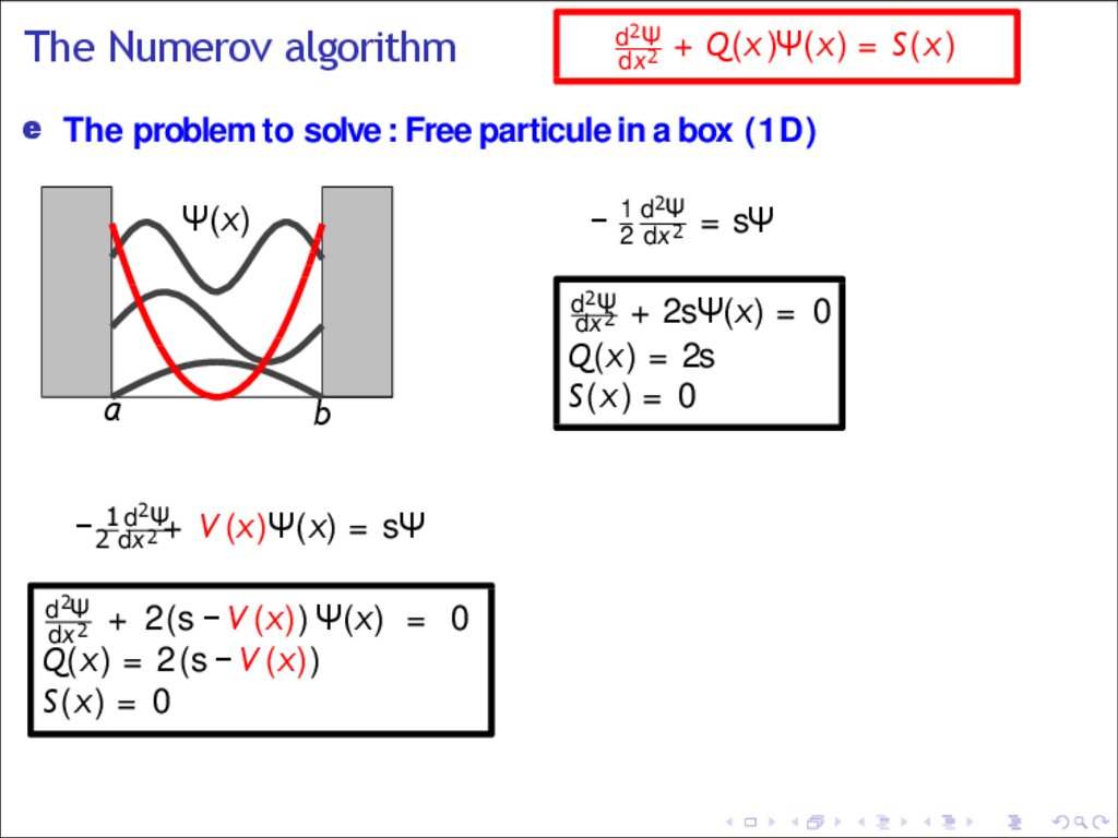
The Numerov algorithme The problem to solve : Free particule in a box (1D)
1 d 2Ψ
Ψ(x)
−2 dx 2 = sΨ
2
d Ψ
−21dx
2 + V (x)Ψ(x ) = sΨ
a
b
This differential equation belongs to the general kind of 2nd order
linear differential equation
d2 Ψ
dx 2
+ Q(x )Ψ(x ) = S(x )
where Q(x ) and S(x ) are continuous functions on a domain [a, b].
The equation is to be solved as a boundary value problem, i.e., Ψ(a)
and Ψ(b) are given.
10.
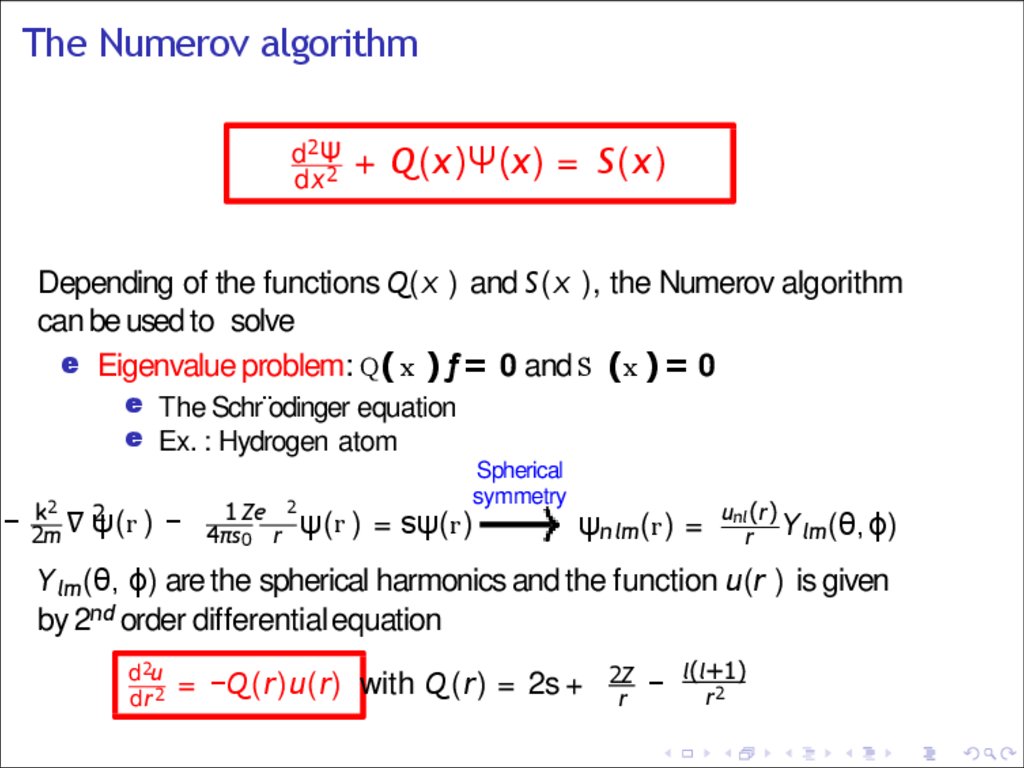
The Numerov algorithmd2 Ψ
dx 2
+ Q(x )Ψ(x ) = S(x )
Depending of the functions Q(x ) and S(x ), the Numerov algorithm
can be used to solve
e Eigenvalue problem: Q ( x ) ƒ= 0 and S (x ) = 0
e The Schr¨odinger equation
e Ex. : Hydrogen atom
k2
− 2m ∇ 2ψ(r ) −
1 Ze
4πs0 r
2
Spherical
symmetry
ψ(r ) = sψ(r )
ψnlm(r ) =
unl (r)
r Ylm(θ, ϕ)
Ylm(θ, ϕ) are the spherical harmonics and the function u(r ) is given
by 2nd order differentialequation
d2u
dr 2
= −Q (r)u(r) with Q (r) = 2s +
2Z
r
−
l(l+1)
r2
11.
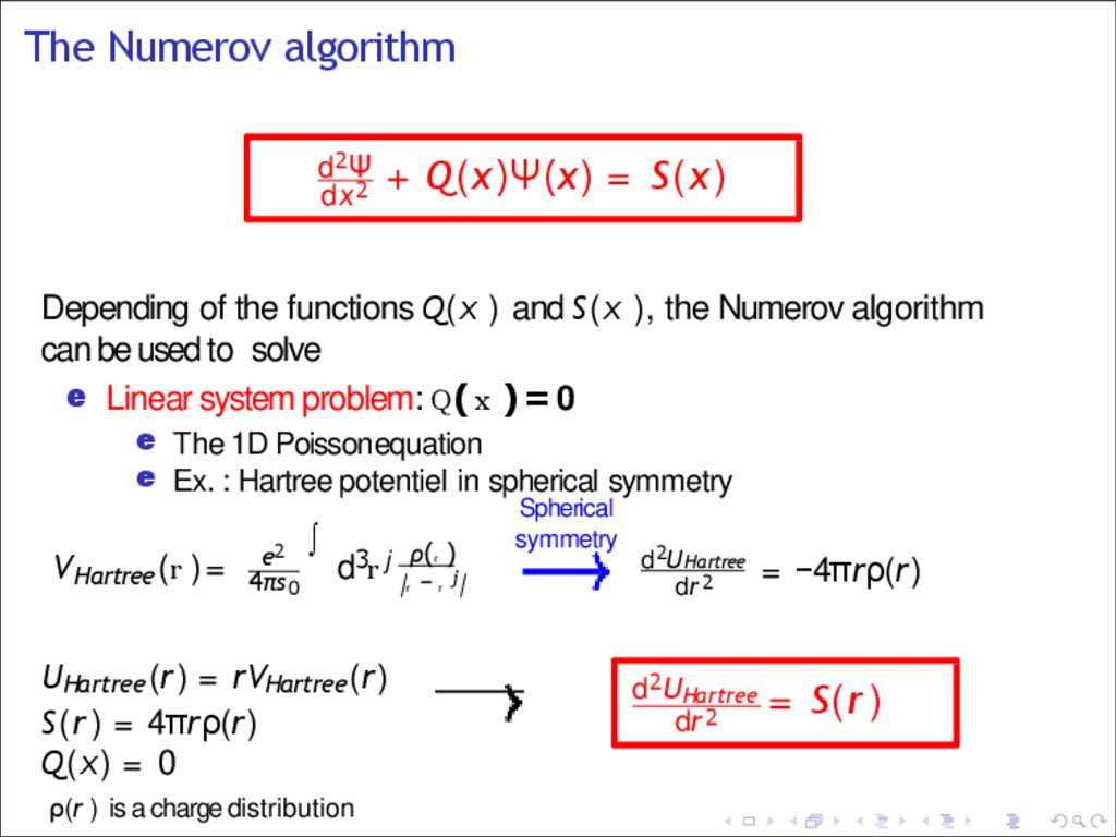
The Numerov algorithmd2 Ψ
dx 2
+ Q(x )Ψ(x ) = S(x )
Depending of the functions Q(x ) and S(x ), the Numerov algorithm
can be used to solve
e Linear system problem: Q ( x ) = 0
e The 1D Poissonequation
e Ex. : Hartree potentiel in spherical symmetry
V Hartree ( r ) =
e2
4πs 0
∫
d3r j | ρ(−
UHartree (r) = rVHartree (r)
S(r ) = 4πrρ(r)
Q(x ) = 0
ρ(r ) is a charge distribution
)
r
r
r
j|
Spherical
symmetry
d2U Hartree
dr 2
d2 UHartree
dr 2
= −4πrρ(r)
= S(r )
12.
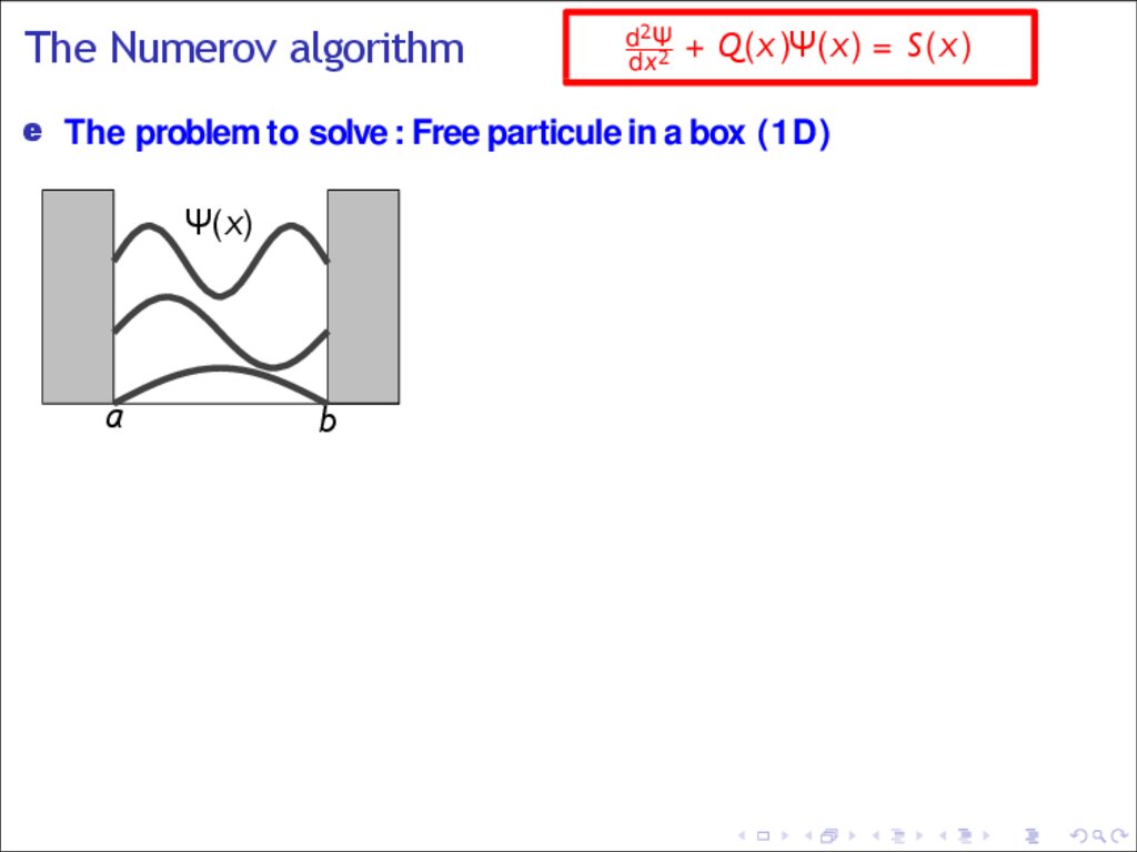
The Numerov algorithmd2Ψ
dx 2
+ Q(x )Ψ(x) = S(x )
e The problem to solve : Free particule in a box (1D)
Ψ(x)
a
b
13.
The Numerov algorithmd2Ψ
dx 2
+ Q(x )Ψ(x) = S(x )
e The problem to solve : Free particule in a box (1D)
− 12 ddxΨ2 = sΨ
2
Ψ(x)
d2Ψ
dx 2
a
b
+ 2sΨ(x) = 0
Q(x ) = 2s
S(x ) = 0
14.
The Numerov algorithmd2Ψ
dx 2
+ Q(x )Ψ(x) = S(x )
e The problem to solve : Free particule in a box (1D)
− 12 ddxΨ2 = sΨ
2
Ψ(x)
d2Ψ
dx 2
a
b
2
d Ψ
−21dx
2 + V (x)Ψ(x) = sΨ
+ 2sΨ(x) = 0
Q(x ) = 2s
S(x ) = 0
15.
The Numerov algorithmd2Ψ
dx 2
+ Q(x )Ψ(x) = S(x )
e The problem to solve : Free particule in a box (1D)
− 12 ddxΨ2 = sΨ
2
Ψ(x)
d2Ψ
dx 2
a
b
2
d Ψ
−21dx
2 + V (x)Ψ(x) = sΨ
d2Ψ
dx 2
+ 2(s −V (x)) Ψ(x) = 0
Q(x ) = 2(s −V (x))
S(x ) = 0
+ 2sΨ(x) = 0
Q(x ) = 2s
S(x ) = 0
16.
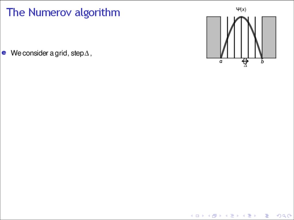
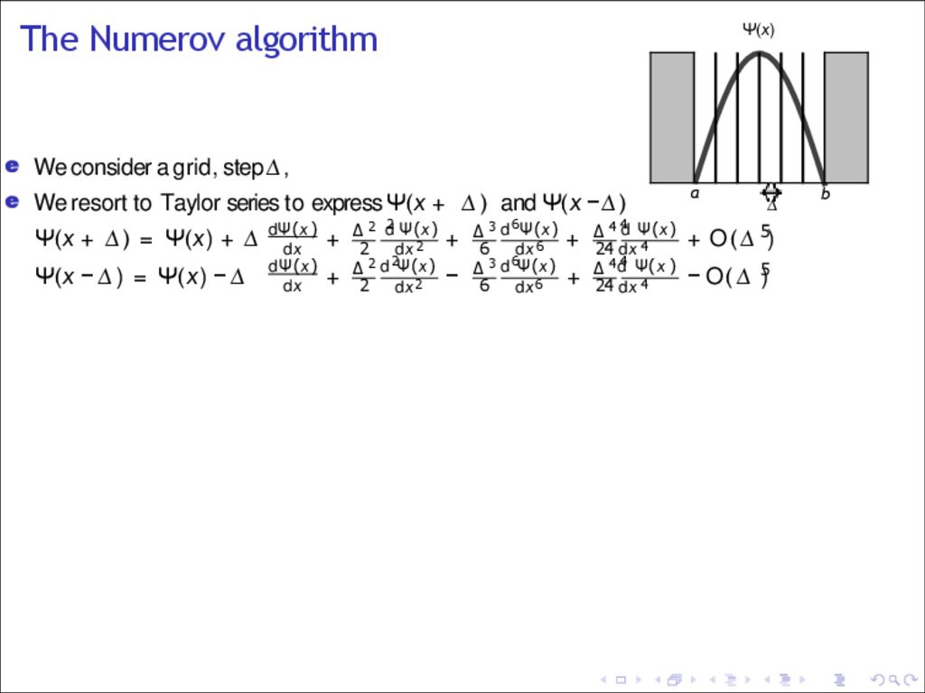
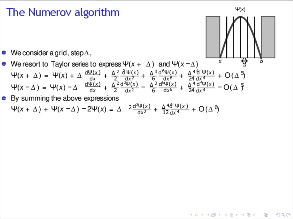
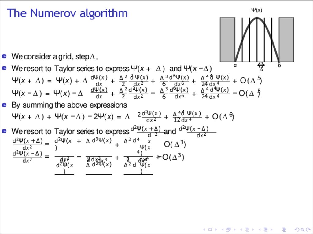
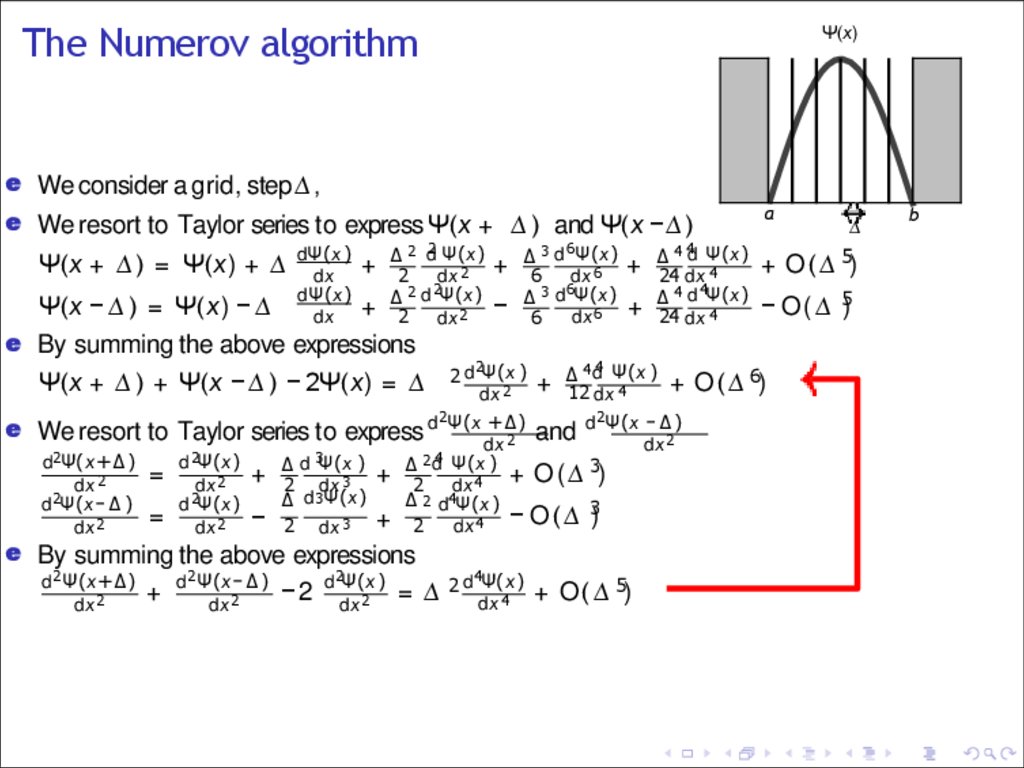
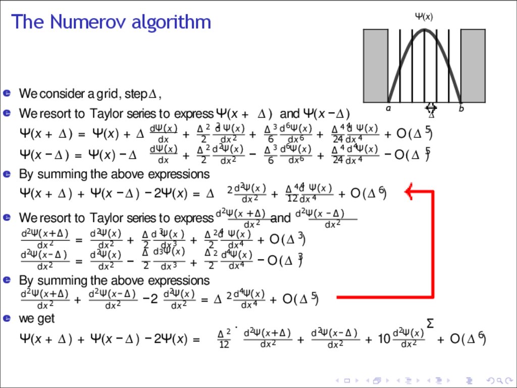
The Numerov algorithmΨ(x)
e We consider a grid, step∆ ,
a
∆
b
17.
The Numerov algorithmΨ(x)
e We consider a grid, step∆ ,
e We resort to Taylor series to express Ψ(x + ∆ ) and Ψ(x −∆ )
Ψ(x + ∆ ) = Ψ(x) + ∆
Ψ(x − ∆ ) = Ψ(x) − ∆
dΨ(x )
dx
dΨ(x )
dx
+
+
∆ 2 d2 Ψ(x)
2
dx 2
2
∆ 2 d Ψ(x )
2
dx 2
+
−
∆3
d 6Ψ(x)
6
dx 6
6
∆ 3 d Ψ(x )
6
dx 6
+
+
4
∆4 d
Ψ(x )
24 dx 4
∆ 4 d4 Ψ(x )
24 dx 4
a
∆
+ O ( ∆ 5)
− O ( ∆ 5)
b
18.
The Numerov algorithmΨ(x)
e We consider a grid, step∆ ,
e We resort to Taylor series to express Ψ(x + ∆ ) and Ψ(x −∆ )
Ψ(x + ∆ ) = Ψ(x) + ∆
Ψ(x − ∆ ) = Ψ(x) − ∆
dΨ(x )
dx
dΨ(x )
dx
+
+
∆ 2 d2 Ψ(x)
2
dx 2
2
∆ 2 d Ψ(x )
2
dx 2
e By summing the above expressions
Ψ(x + ∆ ) + Ψ(x − ∆ ) − 2Ψ(x) = ∆
+
−
∆3
d 6Ψ(x)
6
dx 6
6
∆ 3 d Ψ(x )
dx 6
6
2
2 d Ψ(x )
dx 2
+
+
+
4
∆4 d
Ψ(x )
24 dx 4
4Ψ(x )
4
d
∆
24 dx 4
∆ 4 d4 Ψ(x )
12 dx 4
a
∆
+ O ( ∆ 5)
− O ( ∆ 5)
+ O ( ∆ 6)
b
19.
The Numerov algorithmΨ(x)
e We consider a grid, step∆ ,
e We resort to Taylor series to express Ψ(x + ∆ ) and Ψ(x −∆ )
Ψ(x + ∆ ) = Ψ(x) + ∆
Ψ(x − ∆ ) = Ψ(x) − ∆
dΨ(x )
dx
dΨ(x )
dx
+
+
∆ 2 d2 Ψ(x)
2
dx 2
2
∆ 2 d Ψ(x )
2
dx 2
e By summing the above expressions
Ψ(x + ∆ ) + Ψ(x − ∆ ) − 2Ψ(x) = ∆
+
−
∆3
6
dx 6
6
∆ 3 d Ψ(x )
dx 6
6
2
2 d Ψ(x )
dx 2
2
d 6Ψ(x)
+
+
+
4
∆4 d
Ψ(x )
24 dx 4
4Ψ(x )
4
d
∆
24 dx 4
∆ 4 d4 Ψ(x )
12 dx 4
2
=
dx 22
dx
d2 Ψ(x
)
−
3 3
2
2 dxdx
∆ d3Ψ(x)
+
4)
dx44
2
dx
∆ 2 d Ψ(x
)
+−O(∆ 3 )
∆
+ O ( ∆ 5)
− O ( ∆ 5)
+ O ( ∆ 6)
−∆)
e We resort to Taylor series to express d Ψ(x +∆)
and d Ψ(x dx
2
d 2
3
2
4
2
d Ψ(x + ∆ d Ψ(x)
d Ψ(x +∆)
∆2 d
x
3)
=
+
O(
∆
Ψ(x
)
dx 2
d2Ψ(x − ∆ )
dx 2
a
b
20.
The Numerov algorithmΨ(x)
e We consider a grid, step∆ ,
e We resort to Taylor series to express Ψ(x + ∆ ) and Ψ(x −∆ )
Ψ(x + ∆ ) = Ψ(x) + ∆
Ψ(x − ∆ ) = Ψ(x) − ∆
dΨ(x )
dx
dΨ(x )
dx
+
+
∆ 2 d2 Ψ(x)
2
dx 2
2
∆ 2 d Ψ(x )
2
dx 2
e By summing the above expressions
Ψ(x + ∆ ) + Ψ(x − ∆ ) − 2Ψ(x) = ∆
+
−
∆3
d 6Ψ(x)
6
dx 6
6
∆ 3 d Ψ(x )
dx 6
6
2
2 d Ψ(x )
dx 2
+
+
+
2Ψ(x
dx 2
d 2Ψ(x − ∆ )
=
d 2Ψ(x )
dx 2
d 2Ψ(x )
+
3Ψ(x
)
∆d
2 dx 3
∆ d 3Ψ(x )
2 dx 3
+
Ψ(x )
24 dx 4
4Ψ(x )
4
d
∆
24 dx 4
∆ 4 d4 Ψ(x )
12 dx 4
4
2d
= dx 2 −
+
dx 2
e By summing the above expressions
2
2Ψ(x )
d 2Ψ(x+∆)
∆)
+ d Ψ(x−
−2 d dx
= ∆
2
dx 2
dx 2
4
2 d Ψ(x )
dx 4
+ O ( ∆ 5)
a
∆
+ O ( ∆ 5)
− O ( ∆ 5)
+ O ( ∆ 6)
2
+∆)
−∆)
and d Ψ(x dx
2
dx 2
Ψ(x )
∆
3)
+
O
(
∆
2
dx 4
∆ 2 d4Ψ(x )
− O ( ∆ 3)
2
dx 4
e We resort to Taylor series to express d
d2Ψ(x +∆)
4
∆4 d
b
21.
The Numerov algorithmΨ(x)
e We consider a grid, step∆ ,
e We resort to Taylor series to express Ψ(x + ∆ ) and Ψ(x −∆ )
Ψ(x + ∆ ) = Ψ(x) + ∆
Ψ(x − ∆ ) = Ψ(x) − ∆
dΨ(x )
dx
dΨ(x )
dx
+
+
∆ 2 d2 Ψ(x)
2
dx 2
2
∆ 2 d Ψ(x )
2
dx 2
e By summing the above expressions
Ψ(x + ∆ ) + Ψ(x − ∆ ) − 2Ψ(x) = ∆
+
−
∆3
d 6Ψ(x)
6
dx 6
6
∆ 3 d Ψ(x )
dx 6
6
2
2 d Ψ(x )
dx 2
+
+
+
4
∆4 d
Ψ(x )
24 dx 4
4Ψ(x )
4
d
∆
24 dx 4
∆ 4 d4 Ψ(x )
12 dx 4
a
∆
b
+ O ( ∆ 5)
− O ( ∆ 5)
+ O ( ∆ 6)
2Ψ(x
2
+∆)
−∆)
and d Ψ(x dx
2
dx 2
Ψ(x )
∆
3)
+
O
(
∆
2
dx 4
∆ 2 d4Ψ(x )
− O ( ∆ 3)
2
dx 4
e We resort to Taylor series to express d
d2Ψ(x +∆)
dx 2
d 2Ψ(x − ∆ )
=
d 2Ψ(x )
dx 2
d 2Ψ(x )
+
3Ψ(x
)
∆d
2 dx 3
∆ d 3Ψ(x )
2 dx 3
+
4
2d
= dx 2 −
+
dx 2
e By summing the above expressions
2
2Ψ(x )
4Ψ(x )
d 2Ψ(x+∆)
∆)
+ d Ψ(x−
−2 d dx
= ∆ 2 d dx
+ O ( ∆ 5)
4
2
dx 2
dx 2
e we get
. 2
Σ
2
2Ψ(x )
2
+∆)
−∆)
Ψ(x + ∆ ) + Ψ(x − ∆ ) − 2Ψ(x) = ∆12 d Ψ(x
+ d Ψ(x
+ 10 d dx
+ O ( ∆ 6)
2
dx 2
dx 2
22.
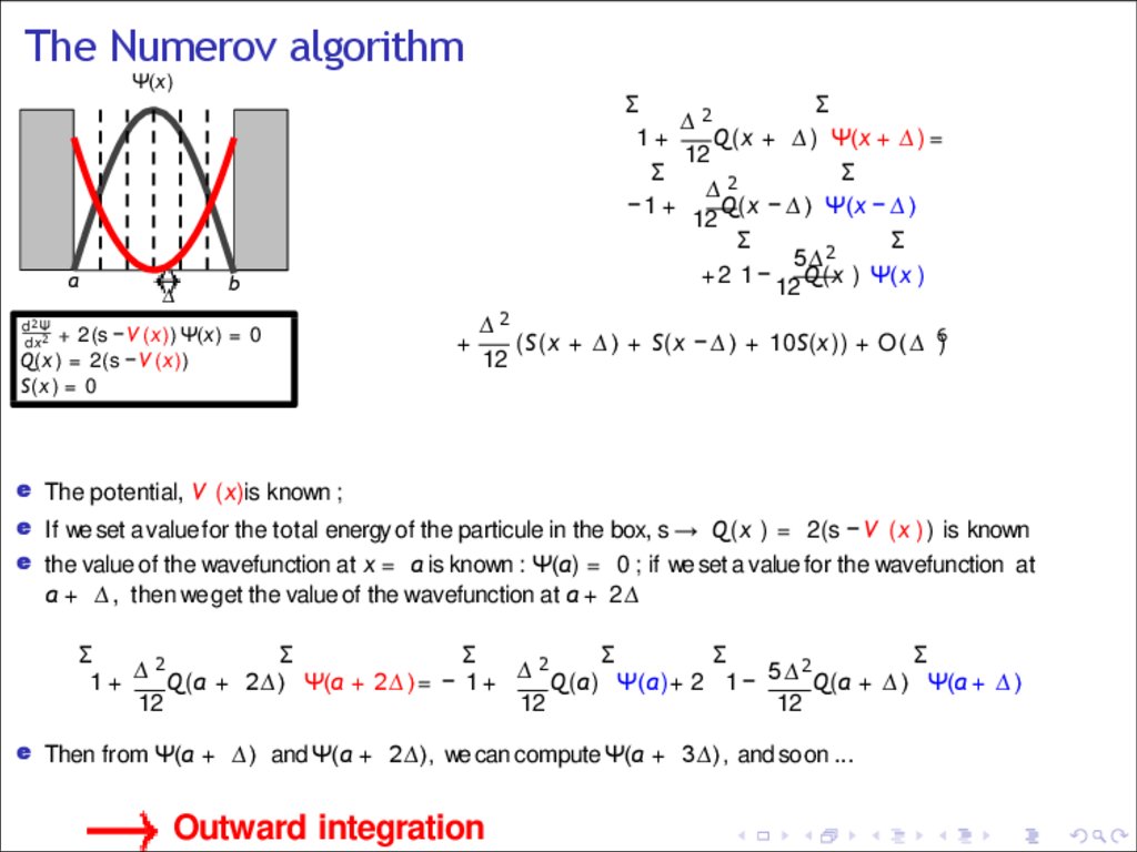
The Numerov algorithme Now from Ψ(x + ∆ ) + Ψ(x − ∆ ) − 2Ψ(x) =
∆2
12
.
d 2Ψ(x+∆)
dx 2
+
d 2Ψ(x − ∆)
dx 2
e Since ddxΨ2 = −Q(x)Ψ(x) + S(x ), we get
e we get
2
Σ
Σ
∆2
1+
Q(x + ∆ ) Ψ(x + ∆ ) =
12
Σ
Σ
∆2
−1+
Q(x − ∆ ) Ψ(x − ∆ )
12
Σ
Σ
5∆ 2
+2 1 − Q(x ) Ψ(x )
12
Ψ(x)
a
d 2Ψ
dx 2
∆
b
∆2
6
+
(S(x + ∆ ) + S(x − ∆ ) + 10S(x )) + O ( ∆ )
12
+ 2 (s − V (x )) Ψ(x) = 0
Q(x ) = 2 (s − V (x))
S(x ) = 0
2
Ψ(x)
+ 10 d dx
2
Σ
+ O ( ∆ 6)
23.
The Numerov algorithmΨ(x)
a
d 2Ψ
dx 2
∆
Σ
Σ
∆2
1+
Q(x + ∆ ) Ψ(x + ∆ ) =
12
Σ
Σ
∆2
−1+
Q(x − ∆ ) Ψ(x − ∆ )
12
Σ
Σ
5∆ 2
+2 1 − Q(x ) Ψ(x )
12
b
+ 2 (s −V (x )) Ψ(x) = 0
Q(x ) = 2(s −V (x))
S(x ) = 0
+
∆2
(S(x + ∆ ) + S(x − ∆ ) + 10S(x )) + O ( ∆ 6)
12
e The potential, V (x)is known ;
e If we set a value for the total energy of the particule in the box, s → Q(x ) = 2(s − V (x )) is known
e the value of the wavefunction at x = a is known : Ψ(a) = 0 ; if we set a value for the wavefunction at
a + ∆ , then we get the value of the wavefunction at a + 2∆
Σ
Σ
Σ
Σ
Σ
Σ
2
2
2
1 + ∆ Q(a + 2∆) Ψ(a + 2 ∆ ) = − 1 + ∆ Q(a) Ψ(a)+ 2 1 − 5∆ Q(a + ∆ ) Ψ(a + ∆ )
12
12
12
e Then from Ψ(a + ∆ ) and Ψ(a + 2∆), we can compute Ψ(a + 3∆), and so on ...
Outward integration
24.
The Numerov algorithmΨ(x)
a
∆
Σ
Σ
∆2
1+
Q(x + ∆ ) Ψ(x + ∆ ) =
12
Σ
Σ
∆2
−1+
Q(x − ∆ ) Ψ(x − ∆ )
12
Σ
Σ
5∆ 2
+2 1 − Q(x ) Ψ(x )
12
b
d 2Ψ
dx 2
+ 2 (s −V (x )) Ψ(x) = 0
Q(x ) = 2(s −V (x))
S(x ) = 0
+
∆2
(S(x + ∆ ) + S(x − ∆ ) + 10S(x )) + O ( ∆ 6)
12
e The potential, V (x)is known ;
e If we set a value for the total energy of the particule in the box, s → Q(x ) = 2(s − V (x )) is known
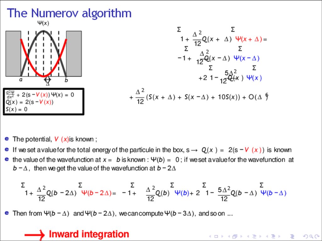
e the value of the wavefunction at x = b is known : Ψ(b) = 0 ; if we set a value for the wavefunction at
b − ∆ , then we get the value of the wavefunction at b − 2∆
Σ
Σ
Σ
2
1 + ∆ Q(b − 2∆) Ψ(b − 2 ∆ ) = − 1 +
12
Σ
Σ
Σ
∆ 2 Q(b) Ψ(b)+ 2 1 − 5∆ 2 Q(b − ∆ ) Ψ(b − ∆ )
12
12
e Then from Ψ(b − ∆ ) and Ψ(b − 2∆), we can compute Ψ(b − 3∆), and so on ...
Inward integration
25.
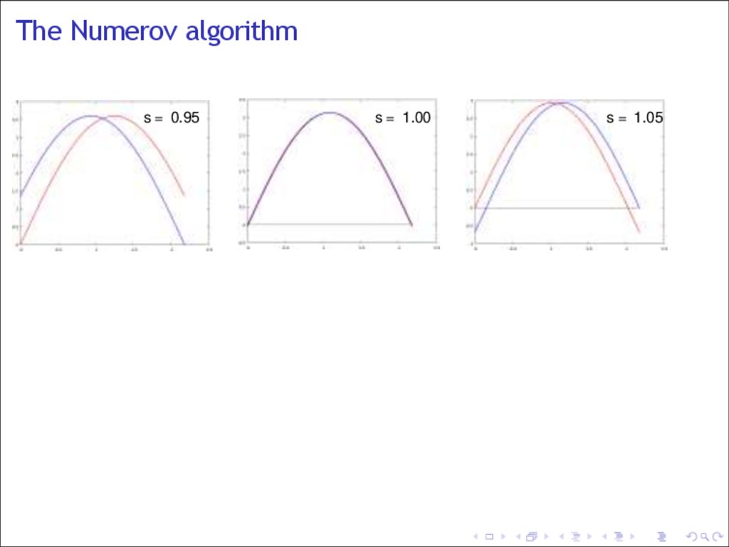
The Numerov algorithmΨ(x)
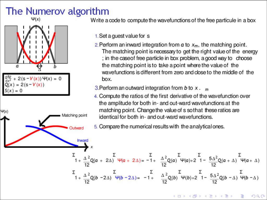
Write a code to compute the wavefunctions of the free particule in a box
1. Set a guest value for s
2. Perform an inward integration from a to xm, the matching point.
a
∆
The matching point is necessary to get the right value of the energy
; in the case of free particle in box problem, a good way to choose
the matching point is to take a point where the value of the
wavefunctions is different from zero and close to the middle of the
box.
b
d 2Ψ
dx 2
+ 2 (s −V (x )) Ψ(x) = 0
Q(x ) = 2(s −V (x))
S(x ) = 0
3.Perform an outward integration from b to x .
m
4. Compute the ratios of the first derivative of the wavefunction over
Ψ(x)
the amplitude for both in- and out-ward wavefunctions at the
matching point. Change the value of s so that these ratios are
identical for both in- and out-ward wavefunctions.
Matching point
5. Compare the numerical results with the analyticalones.
Outward
Inward
x
Σ
Σ
Σ
Σ
Σ
Σ
2
2
2
1 + ∆ Q(a + 2∆) Ψ(a + 2 ∆ ) = − 1 + ∆ Q(a) Ψ(a)+2 1 − 5∆ Q(a + ∆ ) Ψ(a + ∆ )
12
12
12
Σ
Σ
Σ
2
1 + ∆ Q(b − 2∆) Ψ(b − 2 ∆ ) = − 1 +
12
Σ
Σ
Σ
∆ 2 Q(b) Ψ(b)+2 1 − 5∆ 2 Q(b − ∆ ) Ψ(b − ∆ )
12
12
26.
The Numerov algorithms = 0.95
s = 1.00
s = 1.05
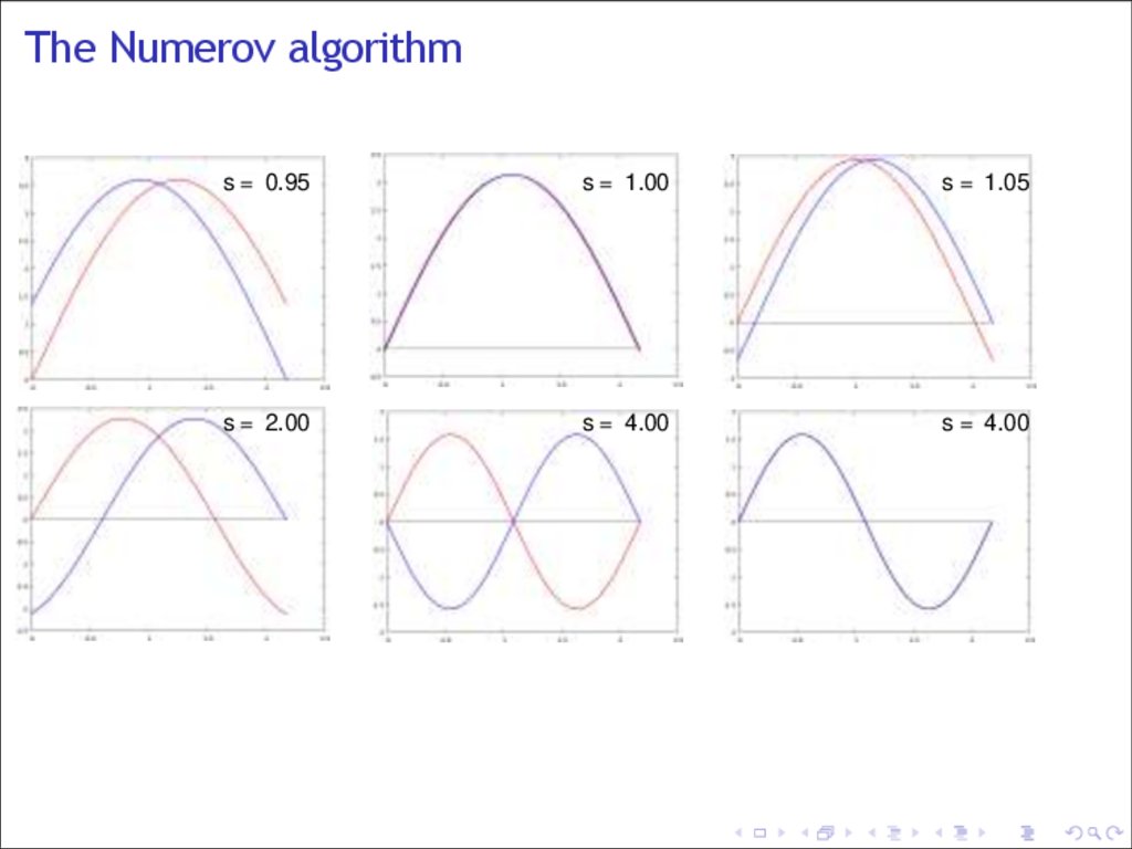
27.
The Numerov algorithms = 0.95
s = 1.00
s = 1.05
s = 2.00
s = 4.00
s = 4.00
28.
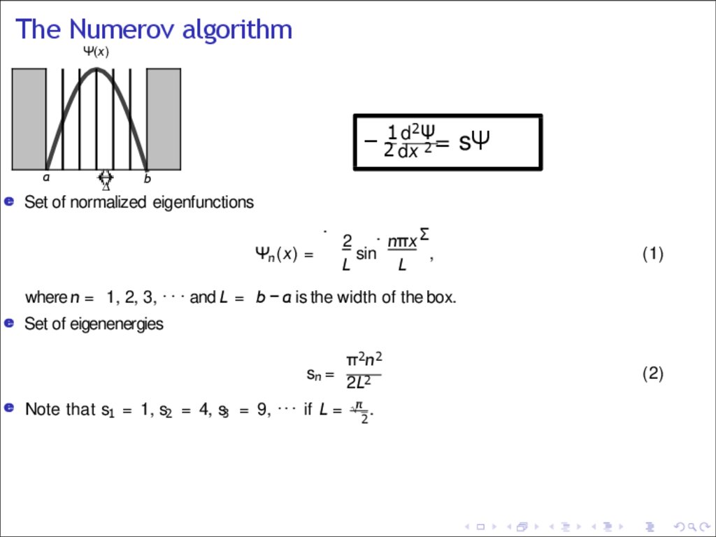
The Numerov algorithmΨ(x)
2
d Ψ
− 21dx
2 = sΨ
a
∆
b
e Set of normalized eigenfunctions
.
Ψn (x) =
2 . nπx Σ
sin
,
L
L
(1)
where n = 1, 2, 3, · · · and L = b − a is the width of the box.
e Set of eigenenergies
sn =
e Note that s1 = 1, s2 = 4, s3 = 9, · · · if L =
π2n2
2L2
√π .
2
(2)