Adomian decomposition method for solving twodimensional nonlinear Volterra fuzzy integral equations

1.

RESEARCH ARTICLE | DECEMBER 10 2018
Adomian decomposition method for solving twodimensional nonlinear Volterra fuzzy integral equations
Artan Alidema; Atanaska Georgieva 
AIP Conf. Proc. 2048, 050009 (2018)
https://doi.org/10.1063/1.5082108
 
View
Online
CrossMark
Export
Citation
09 March 2024 19:34:42

2.

Adomian decomposition method for solving two-dimensional
nonlinear Volterra fuzzy integral equations
Artan Alidema1,b) and Atanaska Georgieva2,a)
2
1
FMNS, University of Prishtina ”Hasan Prishtina”, str. Nena Tereze 1000, Prishtina, Kosovo
Faculty of Mathematics and Informatics, University of Plovdiv ”Paisii Hilendarski”, 24 Tzar Asen, 4000 Plovdiv,
Bulgaria
a)
Corresponding author: [email protected]
b)
[email protected]
Abstract. A numerical method for solving two-dimensional nonlinear Volterra fuzzy integral equation (2D-NVFIE) of the second
kind will is introduced. We convert a nonlinear Volterra fuzzy integral equation to a nonlinear system of Volterra integral equation
in crisp case. We use Adomian Decomposition Method (ADM) to find the approximate solution of this system and hence obtain
an approximation for fuzzy solution of the nonlinear Volterra fuzzy integral equation. Also, the existence and uniqueness of the
solution and convergence of the proposed method are proved. Some numerical examples are included to demonstrate the validity
and applicability of the proposed technique.
The fuzzy differential and integral equations are one of the important part of the fuzzy analysis theory that play major
role in numerical analysis. The concept of integration of fuzzy functions has been introduced by Dubois and Prade
[8], Goetschel and Voxman [16], Kaleva [18] and others. The first applications of fuzzy integration was given by Wu
and Ma who investigated the fuzzy Fredholm integral equation of the second kind.
The study of fuzzy integral equations begins in Kaleva [18], Seikkala [24] and Mordeson and Newman [19],
such integral equations being applied in control mathematical models. The problems posed in the study of fuzzy
integral equations are: existence and uniqueness, boundedness of the solutions [10, 11, 14] and the construction of
numerical methods for the approximate solution.
The existing numerical methods for fuzzy integral equations are based on various techniques: successive approximations and iterative methods [7, 12, 15], analytic-numeric methods like Adomian decomposition, homotopy
analysis and homotopy perturbation [3, 6, 13], quadrature rules and Nystrom techniques [23], Bernstein polynomials
[20], Chebyshev polynomials [5], fuzzy differential transforms [22], expansion methods such as fuzzy collocation,
Galerkin techniques and Taylor series [17].
Adomian decomposition method (ADM) has been recently intensively studied by scientists and engineers and
used for solving nonlinear differential and integral problems. The ADM intruduced by Adomian [1, 2] for solving
different kind of functional equations and has been subject of extensive numerical and analytical studies. ADM consist
of decomposing un-knwon function od any equations into a sum of an infinite number of components define by the
decompositon series. The method essentially is a power series method similar to the perturbation technique. Babolian,
Goghary and Abbasbandy [4] used ADM to solve fuzzy Fredholm integral equations, respectively Allahviranloo,
Abbasbandy [3], solved fuzzy system of Fredholm integral equations. Also, Behzadi [6] solving nonlinear fuzzy
Volterra-Fredholm integral equations with ADM.
In this paper we propose ADM for solving two-dimensional nonlinear Volterra fuzzy integral equation (2DZ t
Z s
NVFIE)
u(s, t) = g(s, t) ⊕ (FR)
(FR)
k(s, t, x, y) G(u(x, y)))dxdy,
(1)
c
a
where g, u : A = [a, b]×[c, d] → E are continuous fuzzy-number valued functions and k : A× A → E 1 , G : E 1 → E 1
are continuous functions on E 1 . The set E 1 is the set of all fuzzy numbers.
1
Proceedings of the 44th International Conference on Applications of Mathematics in Engineering and Economics
AIP Conf. Proc. 2048, 050009-1–050009-8; https://doi.org/10.1063/1.5082108
Published by AIP Publishing. 978-0-7354-1774-8/$30.00
050009-1
09 March 2024 19:34:42
INTRODUCTION

3.

The remainder of this paper is organized as follows: in Section 2, we present the basic notations of fuzzy numbers,
fuzzy functions and fuzzy integrals. In Section 3, the parametric from of 2D-NVFIE is introduced and then ADM is
applied for solving this equation. We aim existence and uniqueness of the solution and convergence of the proposed
method in Section 4. Finally, in Section 5, we illustrate the accuracy of method by solving numerical example.
PRELIMINARIES
In this section, we briefly state some definition and results related to fuzzy numbers and fuzzy-number-valued functions, which will be referred throughout this paper.
Definition 1
[16] A fuzzy number is a function u : R → [0, 1] satisfying the following properties:
(i) u is upper semi-continuous on R,
(ii) u(x) = 0 outside of some interval [c, d],
(iii) there are the real numbers a and b with c ≤ a ≤ b ≤ d, such that u is increasing on [c, a], decreasing on [b, d]
and u(x) = 1 for each x ∈ [a, b],
(iv) u is fuzzy convex set i. e. that is u(λx + (1 − λ)y) ≥ min{u(x), u(y)} for all x, y ∈ R and λ ∈ [0, 1].
r∈[0,1]
Lemma 1
[25] The Hausdorff metric has the following properties:
(i) (E 1 , D) is a complete metric space,
(ii) D(u ⊕ w, v ⊕ w) = D(u, v) for all u, v, w ∈ E 1 ,
(iii) D(u ⊕ v, w ⊕ e) ≤ D(u, w) + D(v, e) for all u, v, w, e ∈ E 1 ,
(iv) D(u ⊕ v, 0̃) ≤ D(u, 0̃) + D(v, 0̃) for all u, v ∈ E 1 ,
(v) D(k u, k v) = |k|D(u, v) for all u, v ∈ E 1 , for allk ∈ R.
(vi) D(k1 u, k2 u) = |k1 − k2 |D(u, 0̃) for all k1 , k2 ∈ E 1 , with k1 k2 ≥ 0 and for allu ∈ E 1 .
For any fuzzy-number-valued function f : A → E 1 we can define the functions f (., ., r), f (., ., r) : A → R, by
f (s, t, r) = ( f (s, t))r− , f (s, t, r) = ( f (s, t))r+ for each (s, t) ∈ A, for each r ∈ [0, 1]. These functions are called the left
and right r−level functions of f.
Definition 2
[26] A fuzzy-number-valued function f : A → E 1 is said to be continuous at (s0 , t0 ) ∈ A if for
1
each ε > 0 there is δ > 0 such that D( f (s, t), f (s0 , t0 )) < ε whenever ((s − s0 )2 + (t − t0 )2 ) 2 < δ. If f be continuous for
each (s, t) ∈ A then we say that f is continuous on A. A fuzzy number u ∈ E 1 is upper bound for a fuzzy-number-valued
function f : A → E 1 if f (s, t, r)r ≤ ur− and f (s, t, r) ≤ ur+ for all (s, t) ∈ A, r ∈ [0, 1]. A fuzzy number u ∈ E 1 is lower
bound for a fuzzy number-valued function f : A → E 1 if ur+ ≤ f (s, t, r) and ur− ≤ f (s, t, r) for all (s, t) ∈ A, r ∈ [0, 1].
A fuzzy-number-valued function f : A → E 1 is said to be bounded it has a lower bound and an upper bound.
Lemma 2
[26] If f : A → E 1 is continuous then it is bounded and its supremum sup f (s, t) must exist and
(s,t)∈A
is determined by u ∈ E 1 with ur− = sup f (s, t, r) and ur+ = sup f (s, t, r). A similar conclusion for the infinum is also
(s,t)∈A
(s,t)∈A
true.
On the set C(A, E 1 ) = { f : A → E 1 ; f is continuous} there is defined the metric
D ( f, g) = max D( f (s, t), g(s, t)), for all f, g ∈ C(A, E 1 ). We see that (C(A, E 1 ), D∗ ) is a complete metric space.
∗
(s,t)∈A
050009-2
09 March 2024 19:34:42
The set of all fuzzy numbers is denoted by E 1 . Any real number a ∈ R can be interpreted as a fuzzy number
ã = χ[a] and therefore R ⊂ E 1 .
According to [25] for any 0 < r ≤ 1 we denote the r−level set [u]r = {x ∈ R : u(x) ≥ r} that is a closed
interval and [u]r = [ur− , ur+ ] for all r ∈ [0, 1]. These lead to the usual parametric representation of a fuzzy number,
by an ordered pair of functions (ur− , ur+ ), which satisfies the following properties: ur− is bounded left continuous nondecreasing function over [0, 1], ur+ is bounded left continuous non-increasing function over [0, 1] and ur− < ur+ .
For u, v ∈ E 1 , k ∈ R, the addition and the scalar multiplication
by
( are defined
[kur− , kur+ ], if k ≥ 0
r
r
r
r
r
r
r
r
r
[u ⊕ v] = [u] + [v] = [u− + v− , u+ + v+ ] and [k u] = k.[u] =
for all r ∈ [0, 1].
[kur+ , kur− ], if k < 0
The neutral element respect to ⊕ in E 1 , denoted by 0̃ = χ[0] . The algebraic properties of addition and scalar
multiplication of fuzzy numbers are given in [25].
As a distance between fuzzy numbers we use the Hausdorff metric [25] defined by D(u, v) =
sup max{|ur− − vr− |, |ur+ − vr+ |} for any u, v ∈ E 1 .

4.

Definition 3
[25] Let f : A → E 1 , for ∆nx : a = x0 < x1 < ... < xn = b and ∆ny : c = y0 < y1 < ... <
yn = d, be two partitions of the intervals [a, b] and [c, d], respectively. Let one consider the intermediates points
ξi ∈ [xi−1 , xi ] and η j ∈ [y j−1 , y j ], i = 1, ..., n; j = 1, ..., n, and δ : [a, b] → R+ and σ : [c, d] → R+ . The divisions
P x = ([xi−1 , xi ]; ξi ), i = 1, ..., n, and Py = ([y j−1 , yi ]; η j ), j = 1, ..., n are said to be δ-fine and σ-fine, respectively, if
[xi−1 , xi ] ⊆ (ξi − δ(ξi ), ξi + δ(ξi )) and [y j−1 , y j ] ⊆ (η j − σ(η j ), η j + σ(η j )).
The function f is said to be two-dimensional Henstock integrable to I ∈ E 1 if for every ε > 0 there are functions
n P
n
P
δ : [a, b] → R+ and σ : [c, d] → R+ such that for any δ-fine and σ-fine divisions we have D(
(xi − xi−1 )(y j −y j−1 )
j=1 i=1
P
f (ξi , η j ), I) < ε, where denotes the fuzzy summation. Then, I is called the two-dimensional Henstock integral of f
Rd
Rb
and is denoted by I( f ) = (FH) (FH) f (s, t)dsdt. If the above δ and σ are constant functions, then one recaptures
c
a
the concept of Riemann integral. In this case, I ∈ E 1 will be called two-dimensional integral of f on A and will be
Rd
Rb
denoted by (FR) (FR) f (s, t)dsdt.
c
a
Lemma 3
[21] Let f : A → E 1 , then f is (FH)-integrable if and only if f and f are Henstock integrable for
any r ∈ [0, 1]. Moreover
r
Zb
Zd
Zb
Zd
Zb
Zd
f
(H)
f
(s,
t)dsdt
=
(H)
(FH)
(FH)
(H)
(s,
t,
r)dsdt,
(H)
f
(s,
t,
r)dsdt
.
a
c
a
c
a
c
Also, if f is continuous then f (., ., r) and f (., ., r) are continuous for any r ∈ [0, 1] and consequently, they are Henstock
integrable. Using Lemma 2. we deduce that f is (FH)-integrable.
c
a
c
a
c
a
Lemma 5
[21] If f : A → E 1 is an integrable bounded function then for any fixed (u, v) ∈ A, the function
ϕu,v : A → R+ defined by ϕu,v (s, t) = D( f (u, v), f (s, t)) is Lebesgue integrable on A.
ADM FOR SOLVING 2D-NVFIE
In this section we introduce the parametric form of integral equation (1) and then apply ADM for solving this
equation. For solving in parametric form of equation (1), consider u(s, t, r) = (u(s, t, r), u(s, t, r)) and u(s, t, r) =
(g(s, t, r), g(s, t, r)), 0 ≤ r ≤ 1 and (s, t) ∈ A are parametric form of u(s, t) and g(s, t), respectively. So the parametric
form of equation (1) is as follows:
Z t Zs
u(s, t, r) = g(s, t, r) +
k(s, t, x, y)G(u(x, y, r))dxdy,
u(s, t, r) = g(s, t, r) +
c
a
c
a
Z t Zs
k(s, t, x, y)G(u(x, y, r))dxdy.
Let for (x, y) ∈ A, we have
H(u(x, y, r), u(x, y, r)) = min{G(β) : u(x, y, r) ≤ β ≤ u(x, y, r)},
Then,
F(u(x, y, r), u(x, y, r)) = max{G(β) : u(x, y, r) ≤ β ≤ u(x, y, r)}.
(
k(s, t, x, y)F(u(x, y, r), u(x, y, r)), if k(s, t, x, y) ≥ 0
k(s, t, x, y)G(u(x, y, r)) =
k(s, t, x, y)H(u(x, y, r), u(x, y, r)), if k(s, t, x, y) < 0
(
k(s, t, x, y)H(u(x, y, r), u(x, y, r)), if k(s, t, x, y) ≥ 0
k(s, t, x, y)G(u(x, y, r)) =
k(s, t, x, y)F(u(x, y, r), u(x, y, r)), if k(s, t, x, y) < 0
050009-3
09 March 2024 19:34:42
Lemma 4
[21] If f and g are fuzzy Henstock integrable functions on A and if the function given by
D( f (s, t), g(s, t)) is Lebesgue integrable, then
Zd
Zb
Zd
Zb
Zd
Zb
D (FH) (FH)
f (s, t)dsdt, (FH) (FH) g(s, t)dsdt ≤ (L) (L) D( f (s, t), g(s, t))dsdt.

5.

for a ≤ x ≤ s ≤ b, c ≤ y ≤ t ≤ d and 0 ≤ r ≤ 1. The ADM method is applied to solve 2D-NVFIE. Let for all
a ≤ x ≤ s ≤ b, c ≤ y ≤ t ≤ d and 0 ≤ r ≤ 1 the function G(β) is increasing for β ∈ [u(x, y, r), u(x, y, r)] and
k(s, t, x, y) ≥ 0 . Then the parametric form of the equation (1) is,
Rt Rs
u(s, t, r) = g(s, t, r) +
k(s, t, x, y)G(u(x, y, r))dxdy
c a
(2)
t
s
R R
u(s, t, r) = g(s, t, r) +
k(s, t, x, y)G(u(x, y, r))dxdy.
c a
Now, we explain ADM as a numerical algorithm for approximating solution of this system of nonlinear integral
equations in crisp case. Then, we find approximate solution for u(s, t, r)
The ADM assume an infinite series solution for the unknowns functions (u(s, t, r), u(s, t, r)), given by
∞
∞
X
X
ui (s, t, r), u(s, t, r) =
u(s, t, r) =
ui (s, t, r)
(3)
i=0
i=0
The nonlinear operator G(u(x, y, r)) and G(u(x, y, r)) into an infinite series of polynomials given by
G(u(x, y, r)) =
∞
X
An (u0 (x, y, r), u1 (x, y, r), ..., un (x, y, r)), G(u(x, y, r)) =
n=0
∞
X
An (u0 (x, y, r), u1 (x, y, r), ..., un (x, y, r)),
n=0
where the An = (An , An ), n ≥ 0 are the so-called Adomian polynomial defined by
∞
∞
1 dn X i
1 dn X i
An (u0 , u1 , ..., un ) =
G λ ui , An (u0 , u1 , ..., un ) =
G λ ui
n! dλn i=0
n! dλn i=0
(4)
,
(5)
λ=0
λ=0
09 March 2024 19:34:42
where λ is formal parameter.
Substituting equations (3) and (4) into equation (2) to get
Z t Zs
∞
∞
X
X
un (s, t, r) = g(s, t, r) +
An (u0 (x, y, r), u1 (x, y, r), ..., un (x, y, r))dxdy,
k(s, t, x, y)
n=0
c
∞
X
Z t Zs
un (s, t, r) = g(s, t, r) +
n=0
n=0
a
k(s, t, x, y)
c
a
∞
X
An (u0 (x, y, r), u1 (x, y, r), ..., un (x, y, r))dxdy
n=0
The components un (s, t, r) and un (s, t, r), n ≥ 0 are computed using the following recursive relations
u0 (s, t, r) = g(s, t, r)
Rt Rs
u1 (s, t, r) =
k(s, t, x, y)A0 (u0 (x, y, r))dxdy
c a
...
un+1 (s, t, r) =
Rt Rs
(6)
k(s, t, x, y)An (u0 (x, y, r), u1 (x, y, r), ..., un (x, y, r))dxdy
c a
and
u0 (s, t, r) = g(s, t, r)
Rt Rs
k(s, t, x, y)A0 (u0 (x, y, r))dxdy
u1 (s, t, r) =
un+1 (s, t, r) =
Rt Rs
k(s, t, x, y)An (u0 (x, y, r), u1 (x, y, r), ..., un (x, y, r))dxdy
c a
We approximate u(s, t, r) = (u(s, t, r), u(s, t, r)) by φ (s, t, r) =
n
lim φ (s, t, r) = u(s, t, r) and lim φn (s, t, r) = u(s, t, r)
n→∞
n
(7)
c a
...
n→∞
050009-4
n−1
P
i=0
ui (s, t, r),
φn (s, t, r) =
n−1
P
i=0
ui (s, t, r), where

6.

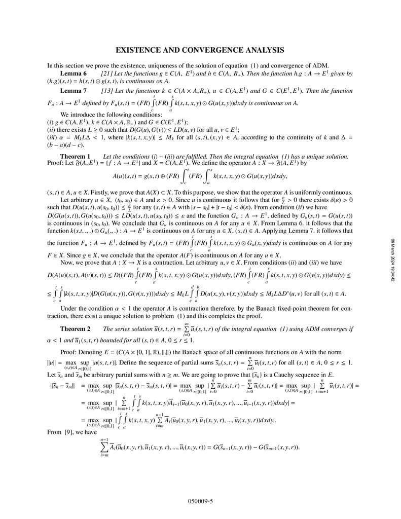
EXISTENCE AND CONVERGENCE ANALYSIS
In this section we prove the existence, uniqueness of the solution of equation (1) and convergence of ADM.
Lemma 6
[21] Let the functions g ∈ C(A, E 1 ) and h ∈ C(A, R+ ). Then the function h.g : A → E 1 given by
(h.g)(s, t) = h(s, t) g(s, t), is continuous on A.
Lemma 7
[13] Let the functions k ∈ C(A × A, R+ ), u ∈ C(A, E 1 ) and G ∈ C(E 1 , E 1 ). Then the function
Rt
Rs
Fu : A → E 1 defined by Fu (s, t) = (FR) (FR) k(s, t, x, y) G(u(x, y))dxdy is continuous on A.
c
a
We introduce the following conditions:
(i) g ∈ C(A, E 1 ), k ∈ C(A × A, R+ ) and G ∈ C(E 1 , E 1 );
(ii) there exists L ≥ 0 such that D(G(u), G(v)) ≤ LD(u, v) for all u, v ∈ E 1 ;
(iii) α = Mk L∆ < 1, where |k(s, t, x, y)| ≤ Mk for all (s, t), (x, y) ∈ A, according to the continuity of k and ∆ =
(b − a)(d − c).
Theorem 1
Let the conditions (i) − (iii) are fulfilled. Then the integral equation (1) has a unique solution.
Proof: Let F(A, E 1 ) = { f : A → E 1 } and X = C(A, E 1 ). We define the operator A : X → F(A, E 1 ) by
Z t
Z s
A(u)(s, t) = g(s, t) ⊕ (FR)
(FR)
k(s, t, x, y) G(u(x, y))dxdy,
c
a
c
a
F ∈ X. Since g ∈ X, we conclude that the operator A(F) is continuous on A for any u ∈ X.
Now, we prove that A : X → X is a contraction. Let arbitrary u, v ∈ X. From conditions (ii) and (iii) we have
Rt
Rs
Rt
Rs
D(A(u)(s, t), A(v)(s, t)) ≤ D((FR) (FR) k(s, t, x, y) G(u(x, y))dxdy, (FR) (FR) k(s, t, x, y) G(v(x, y))dxdy) ≤
c
≤
Rt Rs
a
c
|k(s, t, x, y)|D(G(u(x, y)), G(v(x, y)))dxdy ≤ Mk L
c a
Rd Rb
a
D(u(x, y), v(x, y))dxdy ≤ Mk L∆D∗ (u, v) for all (s, t) ∈ A.
c a
Under the condition α < 1 the operator A is contraction therefore, by the Banach fixed-point theorem for contraction, there exist a unique solution to problem (1) and this completes the proof.
∞
P
Theorem 2
The series solution u(s, t, r) = ui (s, t, r) of the integral equation (1) using ADM converges if
i=0
α < 1 and u1 (s, t, r) bounded for all (s, t) ∈ A, 0 ≤ r ≤ 1.
Proof: Denoting E = (C(A × [0, 1], R), k.k) the Banach space of all continuous functions on A with the norm
n
P
kuk = max sup |u(s, t, r)|. Define the sequence of partial sums sn (s, t, r) =
ui (s, t, r) for all (s, t) ∈ A, 0 ≤ r ≤ 1.
(s,t)∈A r∈[0,1]
i=0
Let sn and sm be arbitrary partial sums with n ≥ m. We are going to prove that {sn } is a Cauchy sequence in E.
n
m
n
P
P
P
ksn − sm k = max sup |sn (s, t, r) − sm (s, t, r)| = max sup | ui (s, t, r) − ui (s, t, r)| = max sup |
ui (s, t, r)| =
(s,t)∈A r∈[0,1]
= max sup |
(s,t)∈A r∈[0,1] i=0
n Rt Rs
P
(s,t)∈A r∈[0,1] i=m+1 c a
Rt Rs
= max sup |
(s,t)∈A r∈[0,1] c a
i=0
(s,t)∈A r∈[0,1] i=m+1
k(s, t, x, y)Ai−1 (u0 (x, y, r), u1 (x, y, r), ..., ui−1 (x, y, r))dxdy| =
k(s, t, x, y)
n−1
P
Ai (u0 (x, y, r), u1 (x, y, r), ..., ui (x, y, r))dxdy|.
i=m
From [9], we have
n−1
X
Ai (u0 (x, y, r), u1 (x, y, r), ..., ui (x, y, r)) = G(sn−1 (x, y, r)) − G(sm−1 (x, y, r)).
i=m
050009-5
09 March 2024 19:34:42
(s, t) ∈ A, u ∈ X. Firstly, we prove that A(X) ⊂ X. To this purpose, we show that the operator A is uniformly continuous.
Let arbitrary u ∈ X, (t0 , s0 ) ∈ A and ε > 0. Since u is continuous it follows that for Lε > 0 there exists δ(ε) > 0
such that D(u(s, t), u(s0 , t0 )) ≤ Lε for any (s, t) ∈ A with |s − s0 | + |t − t0 | < δ(ε). From condition (ii) we have
D(G(u(s, t)), G(u(s0 , t0 ))) ≤ LD(u(s, t), u(s0 , t0 )) ≤ ε and the function Gu : A → E 1 , defined by Gu (s, t) = G(u(s, t))
is continuous in (s0 , t0 ). We conclude that Gu is continuous on A for any u ∈ X. From Lemma 6. it follows that the
function k(s.t, ., .) Gu (., .) : A → E 1 is continuous on A for any u ∈ X, (s, t) ∈ A. Applying Lemma 7. it follows that
Rt
Rs
the function Fu : A → E 1 , defined by Fu (s, t) = (FR) (FR) k(s, t, x, y) Gu (x, y)dxdy is continuous on A for any

7.

So,
Rt Rs
ksn − sm k = max sup |
k(s, t, x, y)[G(sn−1 (x, y, r)) − G(sm−1 (x, y, r))]dxdy| ≤
(s,t)∈A r∈[0,1] c a
Rd Rb
≤ Mk
max sup |G(sn−1 (x, y, r)) − G(sm−1 (x, y, r))|dxdy ≤
c a (x,y)∈A r∈[0,1]
Rd Rb
≤ Mk L
Let, n = m + 1 then
max sup |sn−1 (x, y, r) − sm−1 (x, y, r)|dxdy ≤ Mk L∆ksn−1 − sm−1 k = αksn−1 − sm−1 k
c a (x,y)∈A r∈[0,1]
ksm+1 − sm k ≤ αksm − sm−1 k ≤ α2 ksm−1 − sm−2 k ≤ ... ≤ αm ks1 − s0 k.
Using the triangle inequality we have,
ksn − sm k ≤ hksm+1 − sm k + ksm+2 − sim+1 k + ... + ksn −h sn−1 k ≤
i
n−m
ku1 k.
≤ αm + αm+1 + ... + αn−1 ks1 − s0 k ≤ αm 1 + α + α2 + ... + αn−m−1 ks1 − s0 k ≤ αm 1−α
1−α
n−m
Since 0 < α < 1 so, 1 − α
≤ 1 then
αm
max sup |u1 (s, t, r)|
ksn − sm k ≤
1 − α (s,t)∈A r∈[0,1]
(8)
But |u1 (s, t, r)| ≤ ∞ (since g(s, t, r) is bounded) then ksn − sm k → 0 as m → ∞, from which we conclude that {sn } is a
Cauchy sequence in E. Therefore
u(s, t, r) = lim sn (s, t, r).
(9)
n→∞
Similarly, we have sn is a Cauchy sequence in E, then we can write
u(s, t, r) = lim sn (s, t, r).
(10)
n→∞
u(s, t, r) = (u(s, t, r), u(s, t, r)) = ( lim sn (s, t, r), lim sn (s, t, r)).
n→∞
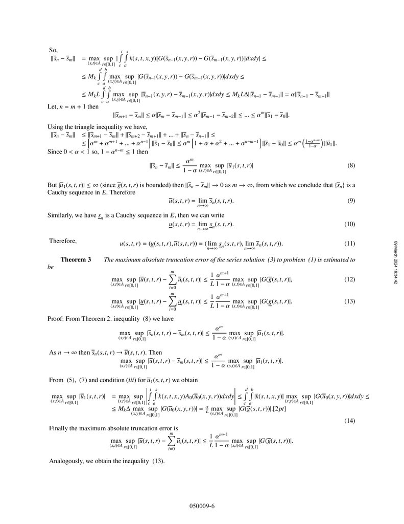
Theorem 3
(11)
n→∞
The maximum absolute truncation error of the series solution (3) to problem (1) is estimated to
be
max sup |u(s, t, r) −
(s,t)∈A r∈[0,1]
max sup |u(s, t, r) −
(s,t)∈A r∈[0,1]
m
X
i=0
m
X
ui (s, t, r)| ≤
1 αm+1
max sup |G(g(s, t, r)|,
L 1 − α (s,t)∈A r∈[0,1]
(12)
ui (s, t, r)| ≤
1 αm+1
max sup |G(g(s, t, r)|.
L 1 − α (s,t)∈A r∈[0,1]
(13)
i=0
Proof: From Theorem 2. inequality (8) we have
max sup |sn (s, t, r) − sm (s, t, r)| ≤
(s,t)∈A r∈[0,1]
αm
max sup |u1 (s, t, r)|.
1 − α (s,t)∈A r∈[0,1]
As n → ∞ then sn (s, t, r) → u(s, t, r). Then
αm
max sup |u(s, t, r) − sm (s, t, r)| ≤
max sup |u1 (s, t, r)|.
(s,t)∈A r∈[0,1]
1 − α (s,t)∈A r∈[0,1]
From (5), (7) and condition (iii) for u1 (s, t, r) we obtain
max sup |u1 (s, t, r)| = max sup
(s,t)∈A r∈[0,1]
Rt Rs
(s,t)∈A r∈[0,1] c a
k(s, t, x, y)A0 (u0 (x, y, r))dxdy ≤
Rd Rb
c a
|k(s, t, x, y)| max sup |G(u0 (x, y, r))|dxdy ≤
(x,y)∈A r∈[0,1]
≤ Mk ∆ max sup |G(u0 (x, y, r))| = αL max sup |G(g(s, t, r))|.[2pt]
(x,y)∈A r∈[0,1]
(s,t)∈A r∈[0,1]
(14)
Finally the maximum absolute truncation error is
m
X
1 αm+1
max sup |u(s, t, r) −
ui (s, t, r)| ≤
max sup |G(g(s, t, r))|.
(s,t)∈A r∈[0,1]
L 1 − α (s,t)∈A r∈[0,1]
i=0
Analogously, we obtain the inequality (13).
050009-6
09 March 2024 19:34:42
Therefore,

8.

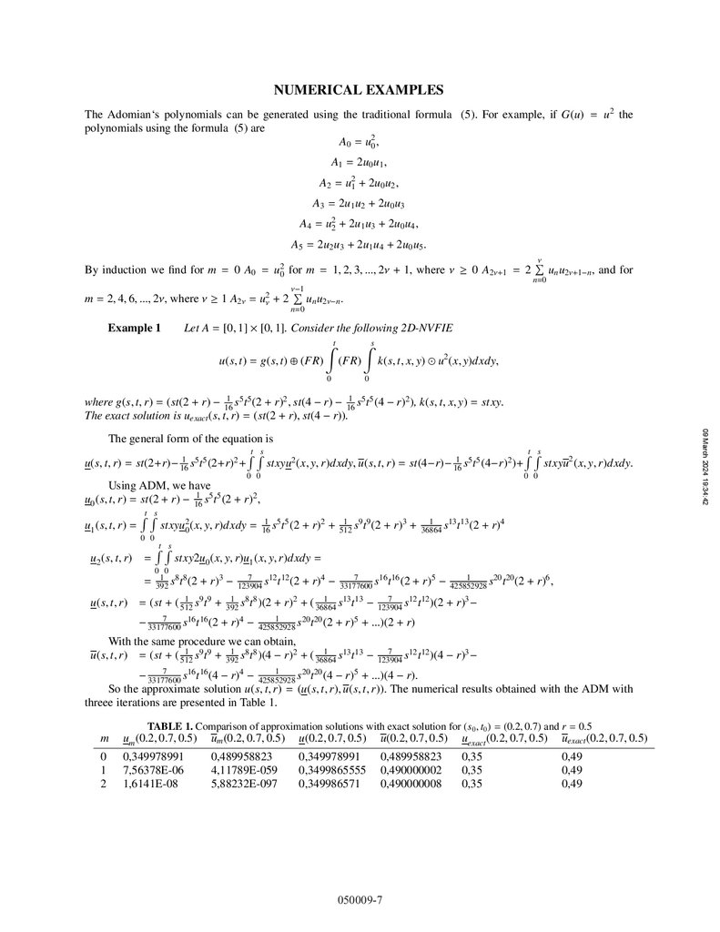
NUMERICAL EXAMPLES
The Adomian‘s polynomials can be generated using the traditional formula (5). For example, if G(u) = u2 the
polynomials using the formula (5) are
A0 = u20 ,
A1 = 2u0 u1 ,
A2 = u21 + 2u0 u2 ,
A3 = 2u1 u2 + 2u0 u3
A4 = u22 + 2u1 u3 + 2u0 u4 ,
A5 = 2u2 u3 + 2u1 u4 + 2u0 u5 .
By induction we find for m = 0 A0 = u20 for m = 1, 2, 3, ..., 2ν + 1, where ν ≥ 0 A2ν+1 = 2
m = 2, 4, 6, ..., 2ν, where ν ≥ 1 A2ν = u2ν + 2
Example 1
ν−1
P
ν
P
un u2ν+1−n , and for
n=0
un u2ν−n .
n=0
Let A = [0, 1] × [0, 1]. Consider the following 2D-NVFIE
Zt
Zs
u(s, t) = g(s, t) ⊕ (FR) (FR) k(s, t, x, y) u2 (x, y)dxdy,
0
0
1 5 5
1 5 5
s t (2 + r)2 , st(4 − r) − 16
s t (4 − r)2 ), k(s, t, x, y) = stxy.
where g(s, t, r) = (st(2 + r) − 16
The exact solution is uexact (s, t, r) = (st(2 + r), st(4 − r)).
0 0
0 0
Using ADM, we have
1 5 5
u0 (s, t, r) = st(2 + r) − 16
s t (2 + r)2 ,
Rt Rs
1 9 9
1
1 5 5
s t (2 + r)2 + 512
s t (2 + r)3 + 36864
s13 t13 (2 + r)4
u1 (s, t, r) =
stxyu20 (x, y, r)dxdy = 16
0 0
u2 (s, t, r) =
Rt Rs
stxy2u0 (x, y, r)u1 (x, y, r)dxdy =
0 0
1 8 8
7
7
1
= 392
s t (2 + r)3 − 123904
s12 t12 (2 + r)4 − 33177600
s16 t16 (2 + r)5 − 425852928
s20 t20 (2 + r)6 ,
u(s, t, r)
1 9 9
1 8 8
1
7
= (st + ( 512
s t + 392
s t )(2 + r)2 + ( 36864
s13 t13 − 123904
s12 t12 )(2 + r)3 −
7
1
− 33177600
s16 t16 (2 + r)4 − 425852928
s20 t20 (2 + r)5 + ...)(2 + r)
With the same procedure we can obtain,
1 9 9
1 8 8
1
7
u(s, t, r) = (st + ( 512
s t + 392
s t )(4 − r)2 + ( 36864
s13 t13 − 123904
s12 t12 )(4 − r)3 −
7
1
− 33177600
s16 t16 (4 − r)4 − 425852928
s20 t20 (4 − r)5 + ...)(4 − r).
So the approximate solution u(s, t, r) = (u(s, t, r), u(s, t, r)). The numerical results obtained with the ADM with
threee iterations are presented in Table 1.
TABLE 1. Comparison of approximation solutions with exact solution for (s0 , t0 ) = (0.2, 0.7) and r = 0.5
m
um (0.2, 0.7, 0.5)
um (0.2, 0.7, 0.5)
u(0.2, 0.7, 0.5)
u(0.2, 0.7, 0.5)
uexact (0.2, 0.7, 0.5)
uexact (0.2, 0.7, 0.5)
0
1
2
0,349978991
7,56378E-06
1,6141E-08
0,489958823
4,11789E-059
5,88232E-097
0,349978991
0,3499865555
0,349986571
0,489958823
0,490000002
0,490000008
0,35
0,35
0,35
0,49
0,49
0,49
050009-7
09 March 2024 19:34:42
The general form of the equation is
Rt Rs
Rt Rs
1 5 5
1 5 5
u(s, t, r) = st(2+r)− 16
s t (2+r)2 +
stxyu2 (x, y, r)dxdy, u(s, t, r) = st(4−r)− 16
s t (4−r)2 )+
stxyu2 (x, y, r)dxdy.

9.

REFERENCES
[1]
[2]
[3]
[4]
[5]
[6]
[7]
[8]
[9]
[10]
[11]
[13]
[14]
[15]
[16]
[17]
[18]
[19]
[20]
[21]
[22]
[23]
[24]
[25]
[26]
050009-8
09 March 2024 19:34:42
[12]
G. Adomian. A review of the decomposition method in applied mathematics. Journal Mathematics Anal App.,
135:501–544, 1988.
G. Adomian. Solving Frontier Problems of Physics. The Decompositon Method. Kluver Academic Publishers, Boston, 12, 1994.
T. Allahvirnaloo, S. Abbasbandy. The Adomian decompositon method applied to fuzzy system of Fredholm
integral equations of the second kind. Int. J. Uncertainty Fuzziness Knowl-Based Systems, 10:101-110, 2006.
E. Babolian, H. S. Goghary ans S. Abbasbandy. Numerical solution of linear Fredholm fuzzy integral equations of the second kind by Adomain method. Applied Math.Comput., 161:733-744, 2005.
A. M. Barkhordari, M. Khezerloo. Fuzzy bivariate Chebyshev method for solving fuzzy Volterra-Fredholm
integral equations. International Journal of Industrial Mathematics, 3:67-77, 2011.
S.S. Behzadi. Solving Fuzzy Nonlinear Volterra-Fredholm Integral Equations by Using Homotopy Analysis
and Adomian Decomposition Methods. International of Fuzzy Set Valued Analysis, 35:13 pages, 2011.
S. S. Behzadi, T. Allahviranloo, S. Abbasbandy. Solving fuzzy second-order nonlinear Volterra-Fredholm
integro-differential equations by using Picard method. Neural Computing and Applications, 21:337-346,
2012.
D. Dubois , and H. Prade. Towards fuzzy differential calculus I,II,III. Fuzzy Sets and Systems, 8:105-116,
225–233, 1982.
I. L. El-Kalla. Convergence of the Adomian method applied to a class of nonlinear integral equations. Journal
Applied Mathematics and Computating, 21:327–376, 2008.
S. Enkov, A. Georgieva, R. Nikolla. Numerical solution of nonlinear Hammerstein fuzzy functional integral
equations. AIP Conference Proceedings, 1789:030006-1-030006-8, 2016.
S. Enkov, A. Georgieva. Numerical solution of two-dimensional nonlinear Hammerstein fuzzy functional
integral equations based on fuzzy Haar wavelets. AIP Conference Proceedings, 1910:050004-1-050004-8,
2017.
S. Enkov, A. Georgieva, A. Pavlova. Quadrature rules and iterative numerical method for two-dimensional
nonlinear Fredholm fuzzy integral equations. Communications in Applied Analysis, 21:479–498, 2017.
A. Georgieva, A. Alidema. Convergence of homotopy perturbation method for solving of two-dimensional
fuzzy Volterra functional integral equations, Advanced Computing in Industrial Mathematics, Studies in
Computational Intelligence, 793, 2019.
A. Georgieva, I. Naydenova. Numerical solution of nonlinear Urisohn-Volterra fuzzy functional integral
equations. AIP Conference Proceedings, 1910:050010-1-050010-8, 2017.
A. Georgieva, A. Pavlova, I. Naydenova. Error estimate in the iterative numerical method for twodimensional nonlinear Hammerstein-Fredholm fuzzy functional integral equations. Advanced Computing
in Industrial Mathematics, Studies in Computational Intelligence, 728:41–45, 2018.
R. Goetschel, W. Voxman. Elementary fuzzy calculus, Fuzzy Sets and Systems, 18:31-43, 1986.
A. Jafarian, N. S. Measoomy, S. Tavan. A numerical scheme to solve fuzzy linear Volterra integral equations
system. J. Appl. Math.: article ID 216923, (2012)
O. Kaleva, Fuzzy differential equations, Fuzzy Sets and Systems, 24:301–317, 1987.
J. Mordeson, W. Newman. Fuzzy integral equations. Information Sciences, 87:215-229, 1995.
M. Mosleh, M. Otadi. Solution of fuzzy Volterra integral equations in a Bernstein polynomial basis, Journal
of Advances in Information Technology, 4:148-155, 2013.
S. Sadatrasoul, R. Ezzati. Numerical solution of two-dimensional nonlinear Hammerstein fuzzy integral
equations based on optimal fuzzy quadrature formula, Journal of Computational and Applied Mathematics, 292:430–446, 2016.
S. Salahshour, T. Allahviranloo. Applicationm of fuzzy differential transform method for solving fuzzyVolterra
integral equations. Applied Mathematical Modelling, 37:1016-1027, 2013.
P. Salehi, M. Nejatiyan. Numerical method for nonlinear fuzzy Volterra integral equations of the second kind.
International Journal of Industrial Mathematics, 3:169-179, 2011.
S. Seikkala On the fuzzy initial value problem, Fuzzy Sets and Systems, 24:319–330, 1987.
C. Wu, Z. Gong. On Henstock integral of fuzzy-number-valued functions(I). Fuzzy Sets and Systems,
120:523–532, 2001.
C. Wu, C. Wu. The supremum and infimum of these to fuzzy-numbers and its applications, J. Math. Anal.
Appl., 210:499–511, 1997.