


 biology
 english
Similar presentations:


. Recent developments of biotechnology in veterinary medicine and animal husbandry")


Quantitative flow cytometry. Advancing the ability of flow cytometry to serve clinical and research purposes
1.
Quantitative Flow Cytometry: advancing the ability of flow cytometryto serve clinical and research purposes
Darya Orlova
28 June, 2016
2.
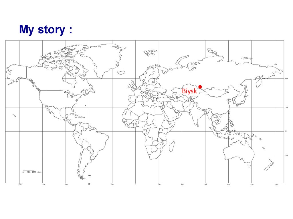
My story :Biysk
3.
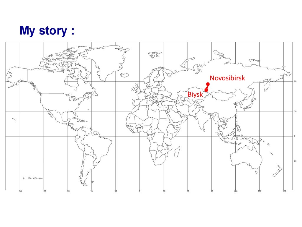
My story :Novosibirsk
Biysk
4.
My story :Novosibirsk
B.S. and M.S. in Physics
5.
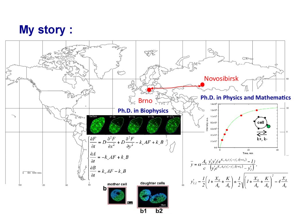
My story :Novosibirsk
Ph.D. in Physics and Mathematics
cell
k+, k-
6.
My story :Novosibirsk
Brno
Ph.D. in Physics and Mathematics
Ph.D. in Biophysics
cell
k+, k-
7.
My story :Novosibirsk
Brno
Stanford, CA
8.
What is the problem?Flow cytometry is an essential tool for basic immunological research,
clinical discovery of potential therapeutics, development and approval of
drugs and devices, disease diagnosis, and therapeutic treatment and
monitoring.
However, the measurements made on different instrument platforms
at different times and places often cannot be compared. Such
discrepancies between and among measurements accompanied by
discrepancies in data analysis procedures introduce uncertainty in
diagnostic decisions, and impedes advances in basic science.
http://www.nist.gov/mml/bbd/bioassay/quantitative_flow_cytometry.cfm
9.
The objective :To develop methods and procedures to enable quantitative
measurements of biological substances such as cells, proteins, etc.
By providing quantitative flow cytometry measurement solutions, we
ensure that researchers can produce better data, better drugs are
developed, and patients get better treatment in a clinical setting.
10.
Accurate classification and enumeration of cells with specificphenotypic characteristics.
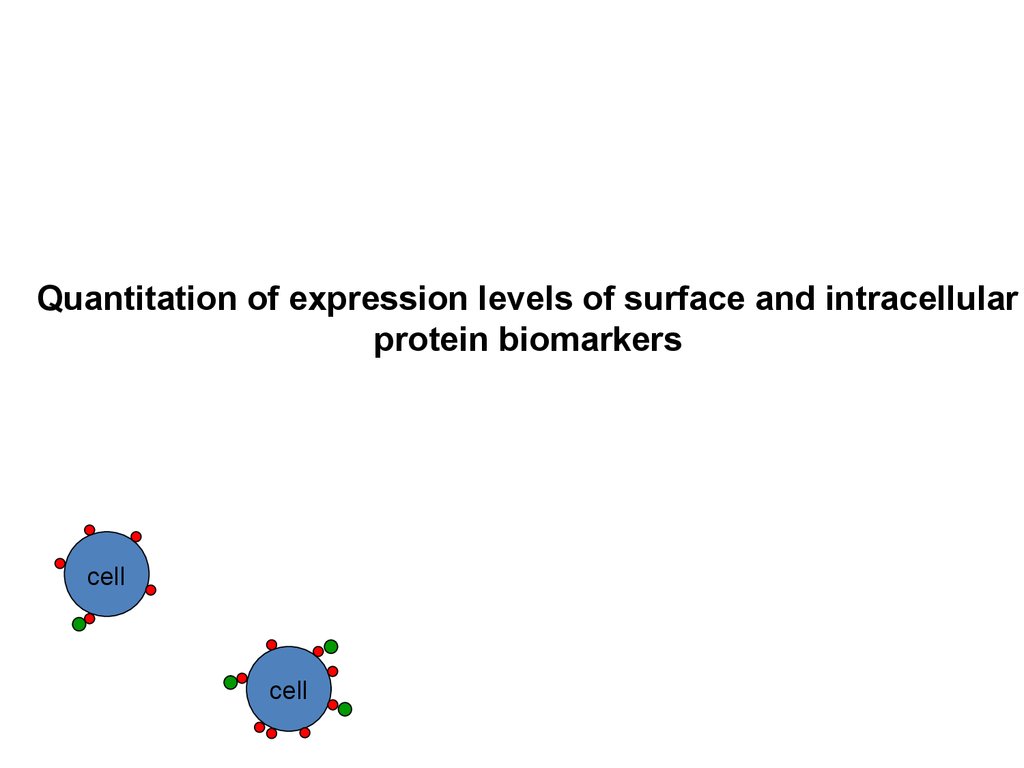
Quantitation of expression levels of surface and intracellular
protein biomarkers.
11.
Classification and enumeration of cells withspecific phenotypic characteristics
Marginal Zone B cells
Follicular
B cells
Immature B + B-1 a cells
12.
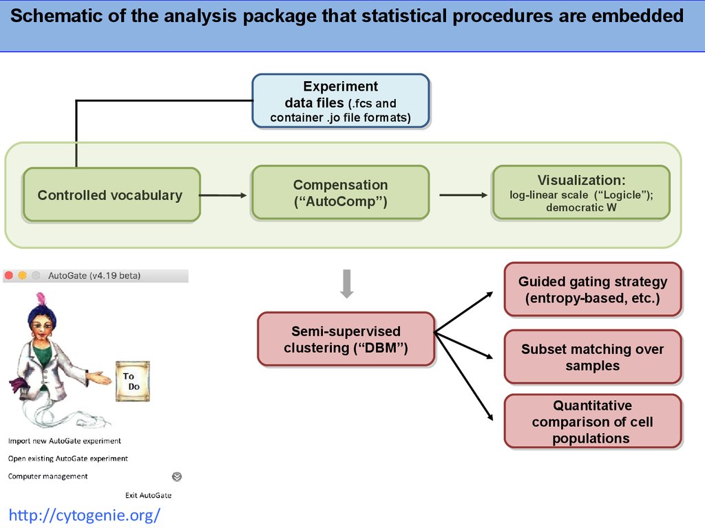
Schematic of the analysis package that statistical procedures are embeddedExperiment
Experiment
data
data files
files (.fcs
(.fcs and
and
container
container .jo
.jo file
file formats)
formats)
Controlled vocabulary
vocabulary
Controlled
Compensation
Compensation
(“AutoComp”)
(“AutoComp”)
Visualization:
Visualization:
log-linear scale
scale (“Logicle”);
(“Logicle”);
log-linear
democratic W
W
democratic
Guided
Guided gating
gating strategy
strategy
(entropy-based,
(entropy-based, etc.)
etc.)
Semi-supervised
Semi-supervised
clustering
clustering (“DBM”)
(“DBM”)
Subset
Subset matching
matching over
over
samples
samples
Quantitative
Quantitative
comparison
comparison of
of cell
cell
populations
populations
http://cytogenie.org/
13.
Projection PursuitHigh Dimensional Data
Dimension Reduction
Visualisation
Classification
Analysis
http://www.few.vu.nl/~tvpham/images/ppde.jpg
Projection pursuit seeks one projection at a time
http://slideplayer.com/slide/4970323/#
14.
Projection Pursuit1-D: 42% of data captured
3-D: 7% of data captured
2-D: 14% of data captured
4-D: 3% of data captured
t=0
http://www.newsnshit.com/curse-of-dimensionalityinteractive-demo/
15.
User-Guided Projection Pursuit16.
Finding clusters by density based merging (DBM)Cluster C
Cluster D
Backg
Cluster
B roundCluster A
Walther G. et al, Adv Bioinformatics, 2009
Cluster E
17.
Myeloid and GranulocytesNeutrophils
Monocytes
Live
Singlets
Eosinophils
Lymphoid cells
Alpha Beta
T cells
Macrophages+DC
T cells
Marginal Zone B cells
Follicular
B cells
Gamma Delta
T cells
B cells
Immature B + B-1 a cells
NK+NKT+DC
NK cells
CD43+NK cells
B-1 a cells
Immature
B cells
18. How different are these two samples?
pSTAT5 kineticsIL2 (stim) 0 min
IL2 (stim) 36 min
19.
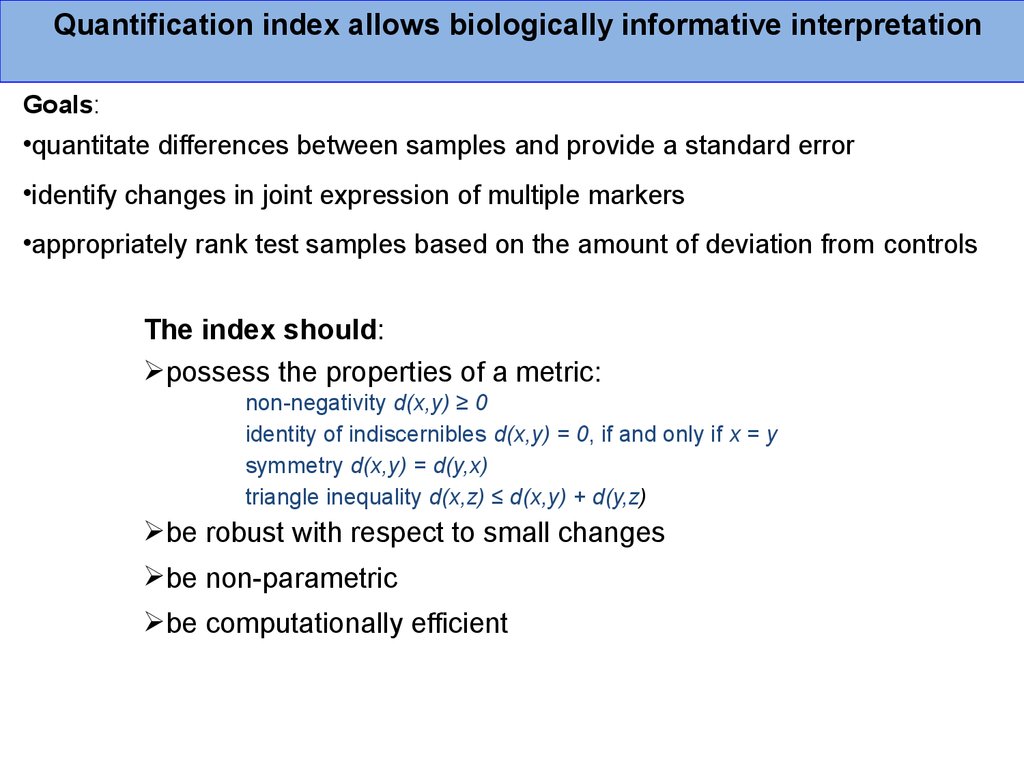
Quantification index allows biologically informative interpretationGoals:
•quantitate differences between samples and provide a standard error
•identify changes in joint expression of multiple markers
•appropriately rank test samples based on the amount of deviation from controls
The index should:
possess the properties of a metric:
non-negativity d(x,y) ≥ 0
identity of indiscernibles d(x,y) = 0, if and only if x = y
symmetry d(x,y) = d(y,x)
triangle inequality d(x,z) ≤ d(x,y) + d(y,z)
be robust with respect to small changes
be non-parametric
be computationally efficient
20.
Most of the current methods ask “Do samples differ?”Some test statistics are limited to univariate data, e.g., KolmogorovSmirnoff statistic and Overton Subtraction (Sheskin, 2000)
Recent methods can be applied to multivariate flow cytometry
• Probability Binning (Roederer et al., 2001)
• Frequency Difference Gating (Roederer and Hardy, 2001)
• Cytometric Fingerprinting (Rogers et al., 2008)
• Quadratic Form Metric (Bernas et al., 2008)
How different are samples?
With respect to both the proportion of cells whose marker expression has
changed and the magnitude of the change
21.
Probability binning plateaus but EMD increases monotonicallyas one population moves further from the center of the other
22.
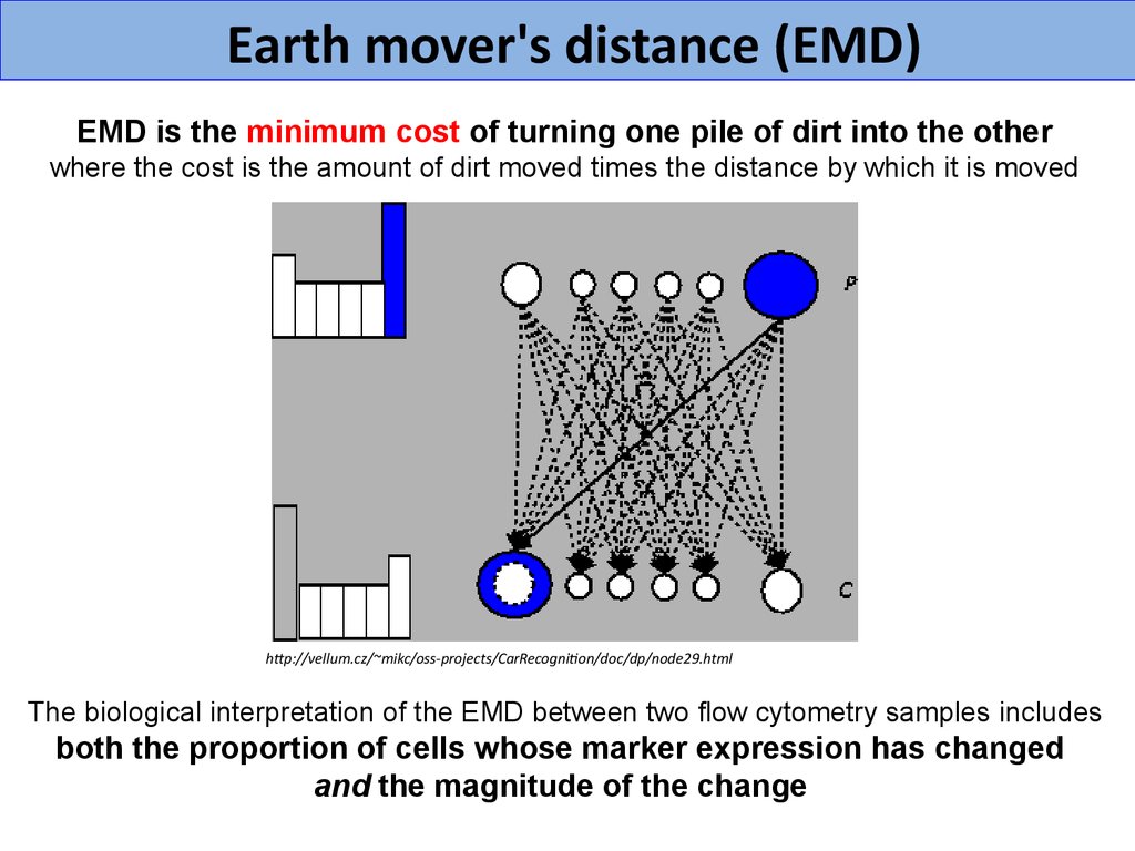
Earth mover's distance (EMD)EMD is the minimum cost of turning one pile of dirt into the other
where the cost is the amount of dirt moved times the distance by which it is moved
http://vellum.cz/~mikc/oss-projects/CarRecognition/doc/dp/node29.html
The biological interpretation of the EMD between two flow cytometry samples includes
both the proportion of cells whose marker expression has changed
and the magnitude of the change
23.
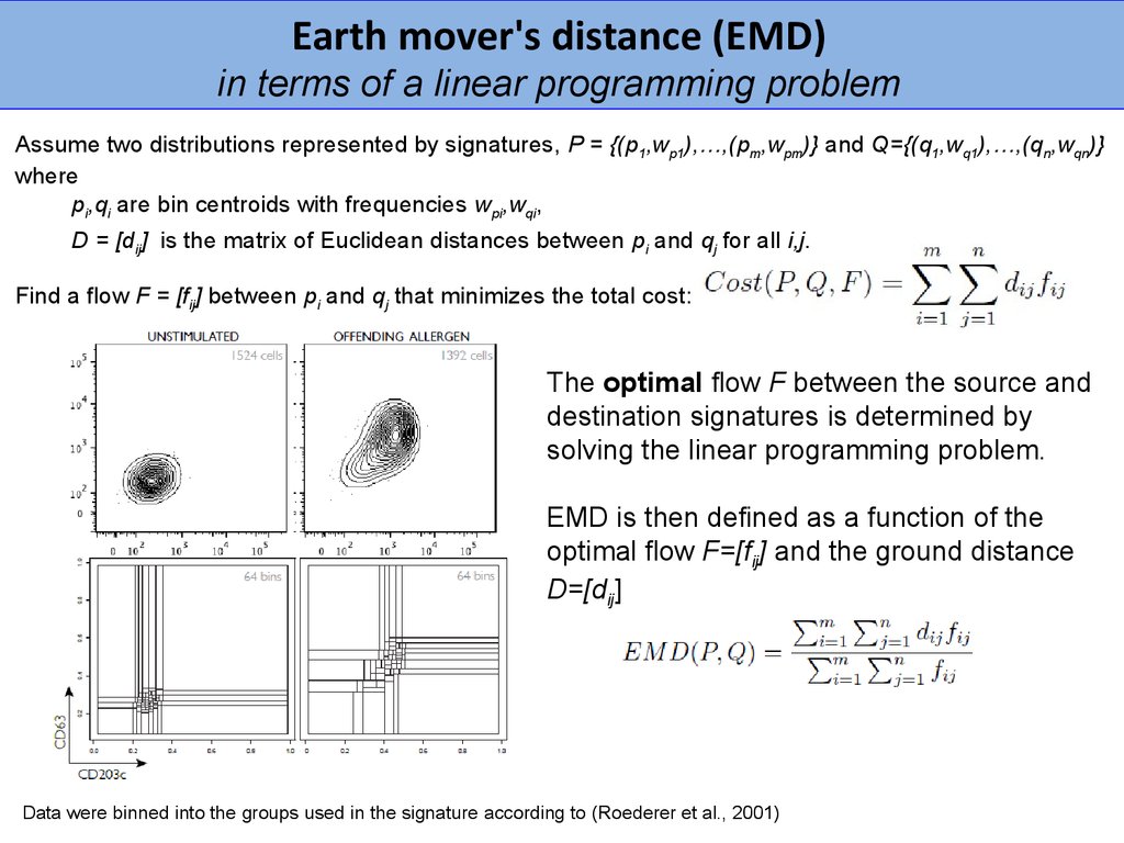
Earth mover's distance (EMD)in terms of a linear programming problem
Assume two distributions represented by signatures, P = {(p1,wp1),…,(pm,wpm)} and Q={(q1,wq1),…,(qn,wqn)}
where
pi,qi are bin centroids with frequencies wpi,wqi,
D = [dij] is the matrix of Euclidean distances between pi and qj for all i,j.
Find a flow F = [fij] between pi and qj that minimizes the total cost:
The optimal flow F between the source and
destination signatures is determined by
solving the linear programming problem.
EMD is then defined as a function of the
optimal flow F=[fij] and the ground distance
D=[dij]
Data were binned into the groups used in the signature according to (Roederer et al., 2001)
24.
Diagnostic tool for distinguishing cystic fibrosis (CF)from allergic bronchopulmonary aspergillosis (ABPA) in CF
Antibiotics
Corticosteroids
Anti-fungal
medicines
Blood basophils from patients with ABPA are
hyper-responsive to stimulation by Af allergen
Surface CD203c in blood basophils after ex vivo stimulation with A. fumigatus (Af) allergen/extract (offending)
or peanut (non offending) allergen. Gernez et al. J Cyst Fibros 11:502-10, 2012
25.
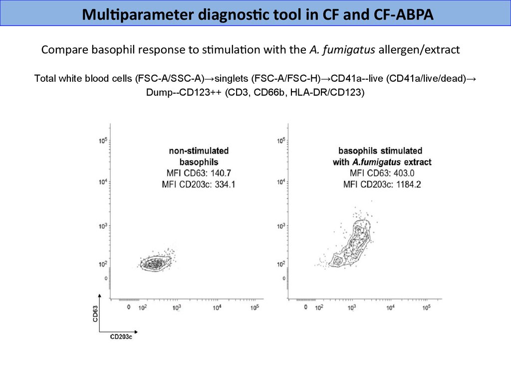
Multiparameter diagnostic tool in CF and CF-ABPACompare basophil response to stimulation with the A. fumigatus allergen/extract
Total white blood cells (FSС-A/SSC-A)→singlets (FSС-A/FSC-H)→CD41a--live (CD41a/live/dead)→
Dump--CD123++ (CD3, CD66b, HLA-DR/CD123)
26.
EMD scores based on expression of two independent flow cytometrymarkers more accurately distinguish allergic (CF-ABPA) from non-allergic
(CF) patients
27.
Cluster matching28.
Quantitation of expression levels of surface and intracellularprotein biomarkers
cell
cell
29.
Antigen-antibody interactions on the surface of cellsWe previously suggested an antigen concentration quantification approach which
utilizes the value of the binding rate constant for each particular monoclonal
antibody-antigen reaction measured with flow cytometry
cell
cell
cell
30.
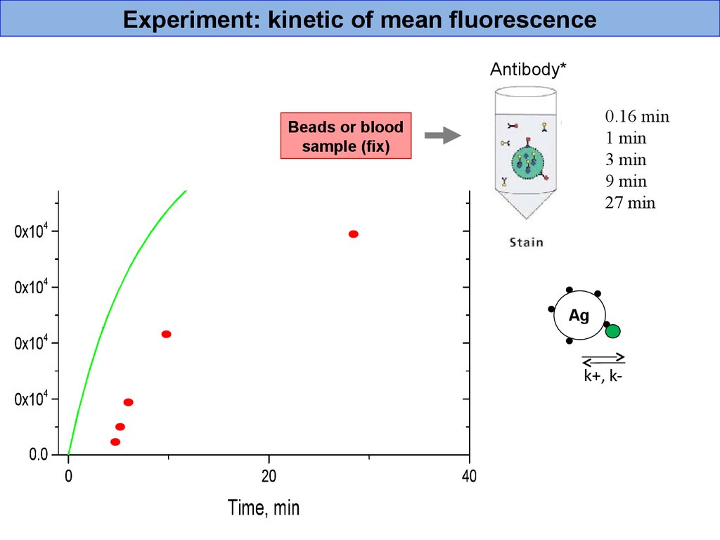
Experiment: kinetic of mean fluorescenceAntibody*
0.16 min
1 min
3 min
9 min
27 min
Beads or blood
sample (fix)
Ag
k+, k-
31.
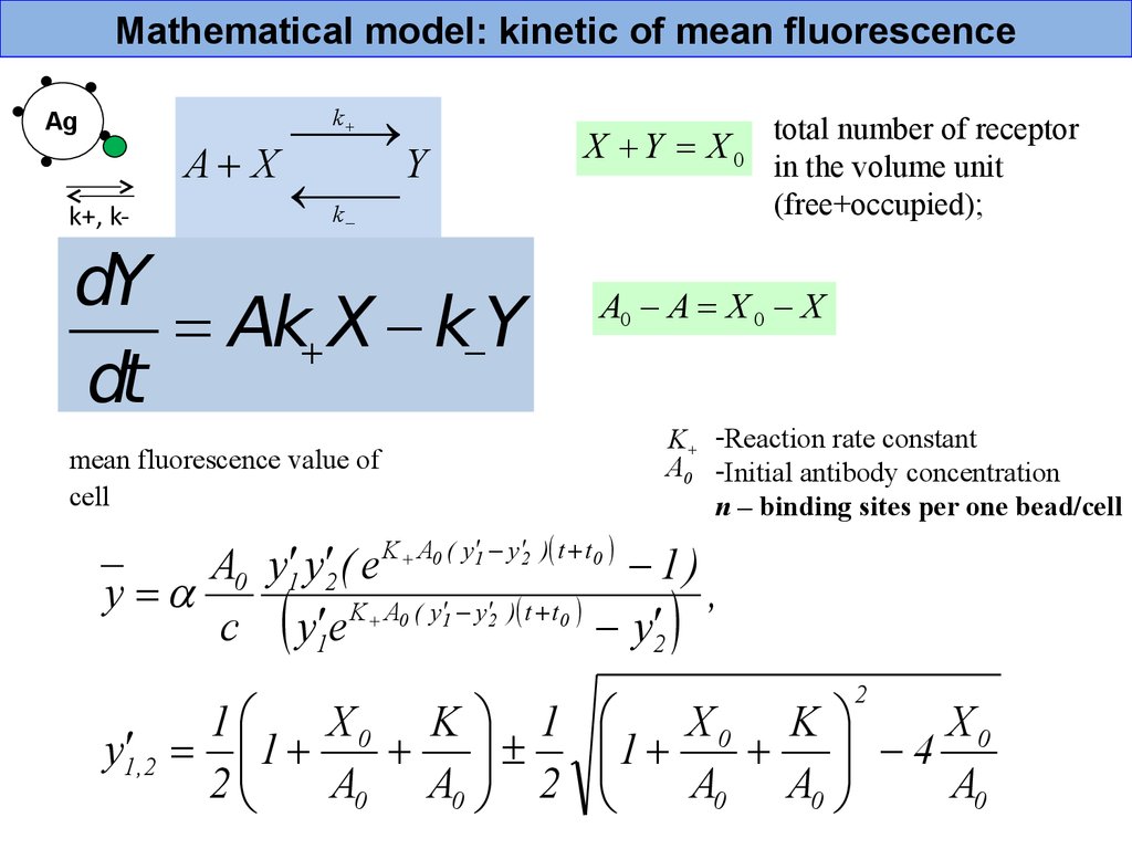
Mathematical model: kinetic of mean fluorescenceA X
Y
k
k
Ag
k+, k-
dY
= Ak X k Y
dt
mean fluorescence value of
cell
X Y = X0
total number of receptor
in the volume unit
(free+occupied);
A0 A = X 0 X
K+ -Reaction rate constant
A0 -Initial antibody concentration
n – binding sites per one bead/cell
K A0 ( y 1 y 2 ) t t 0
A0 y1 y2 ( e
1)
y =
,
K A0 ( y 1 y 2 ) t t 0
c y1 e
y2
1
X0 K 1
y1 ,2 = 1
2
A0 A0 2
2
X0 K
X0
1
4
A0 A0
A0
32.
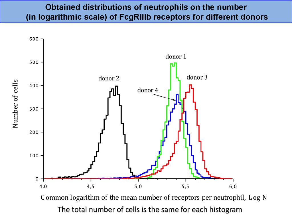
Obtained distributions of neutrophils on the number(in logarithmic scale) of FcgRIIIb receptors for different donors
The total number of cells is the same for each histogram
33.
However, application of such rate constant approach is currently limitedby the lack of measured binding rate constant values for most antigenantibody pairs of interest and changes in experimental conditions
k+, k- (temperature, viscosity, fluorescent labels, etc.)
Ag
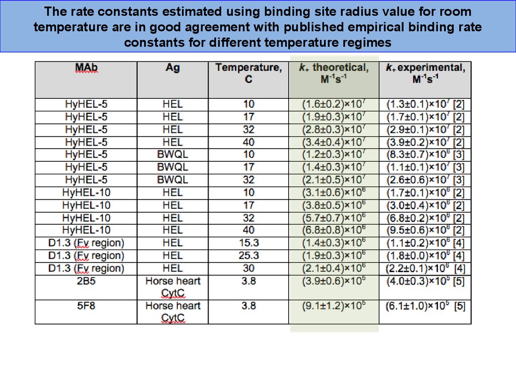
As a solution to this problem we introduce a theoretical approach allowing
predicting the binding rate constant for changes in experimental conditions.
We verify our theoretical approach comparing the results to experimentally
measured binding rate constants for classical examples of monoclonal
antibody-antigen interactions under different temperature regimes.
34.
Agk+, k-
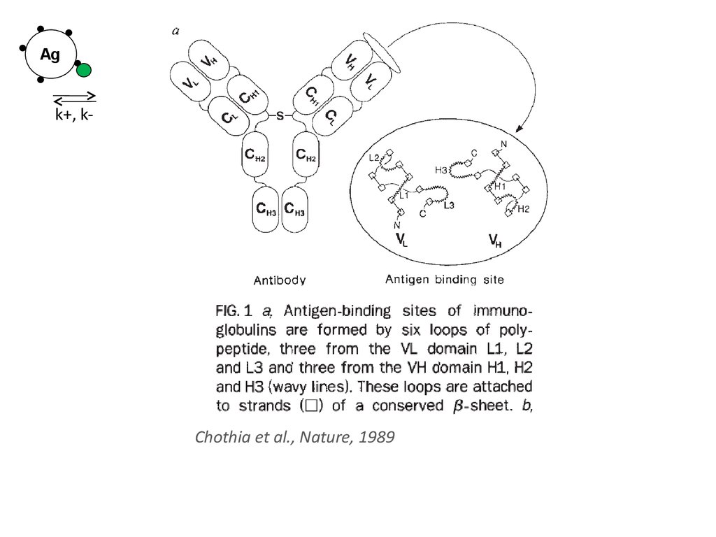
Chothia et al., Nature, 1989
35.
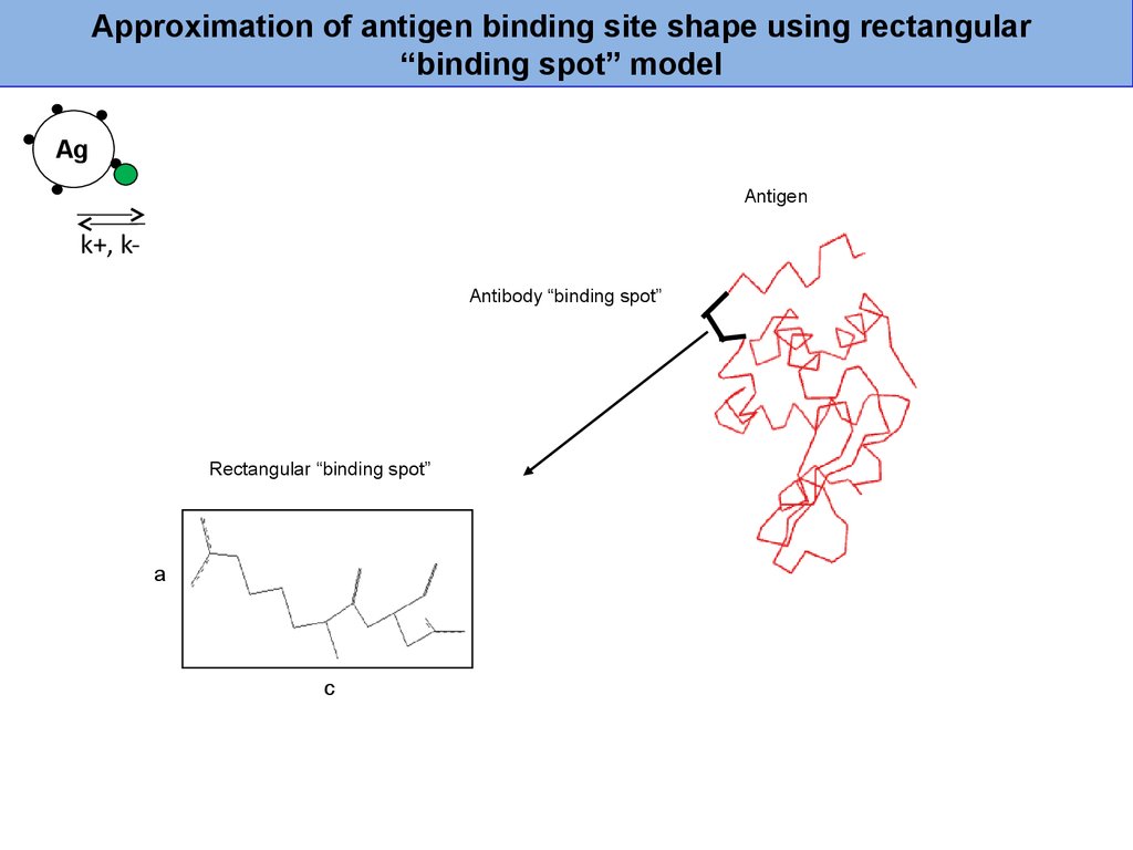
Approximation of antigen binding site shape using rectangular“binding spot” model
Ag
Antigen
k+, kAntibody “binding spot”
Rectangular “binding spot”
a
c
36.
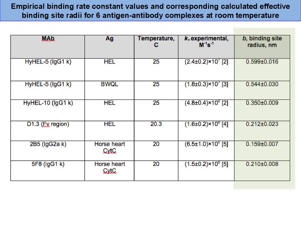
From the binding rate constant k+, it was possible to estimate the radius b ofthe binding site (a circular approximation of the shape of the site placed on a
spherical reagent) using following expression
k BT b
k = N1 N 2
12
3
1
1
R1 R2
3
where is the viscosity of the media, kB is the Boltzmann constant, T is the
temperature; R1 and R2 are radii, N1 and N2 are valences of the first and
second reactants, correspondingly.
The radius of antibody molecules can be estimated from the diffusion
coefficient using Stokes–Einstein equation : D = k B T
6 R
On the other hand, the diffusion coefficient of the molecule can be estimated
using the known relationship between the diffusion coefficient (in cm 2 s-1) and
the molar mass (in Da), M, of a protein (in water at room temperature)
LogM = 16.88 3.51 LogD
37.
Empirical binding rate constant values and corresponding calculated effectivebinding site radii for 6 antigen-antibody complexes at room temperature
38.
The rate constants estimated using binding site radius value for roomtemperature are in good agreement with published empirical binding rate
constants for different temperature regimes
39.
Electrical analogueAg
k+, k-
Physics of chemoreception. HC Berg & EM Purcell, Biophys J 20, 93-219 (1977).
40.
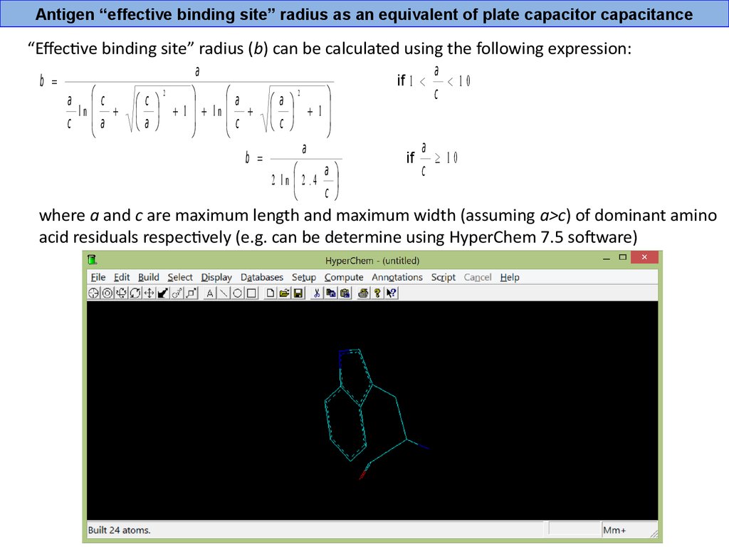
Antigen “effective binding site” radius as an equivalent of plate capacitor capacitance“Effective binding site” radius (b) can be calculated using the following expression:
b =
a с
ln
с a
a
2
a
с
1 ln
c
a
2
a
1
c
a
b =
a
2 ln 2 .4
c
if 1 <
if
a
< 10
c
a
³ 10
c
where a and c are maximum length and maximum width (assuming a>c) of dominant amino
acid residuals respectively (e.g. can be determine using HyperChem 7.5 software)
41.
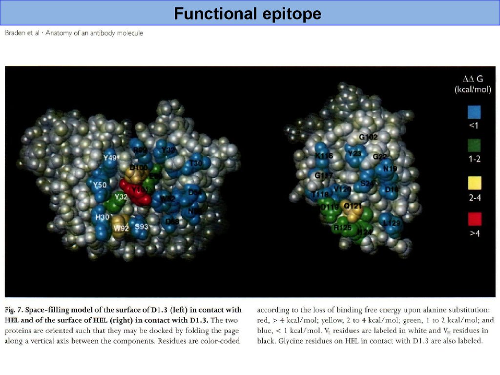
Functional epitope42.
Comparison of estimates for binding site radius electrostatic analogues witheffective binding site radii calculated using empirical rate constant values
43.
The rate constants estimated using binding site radius value for roomtemperature are in good agreement with published empirical binding rate
constants for different temperature regimes
*
44.
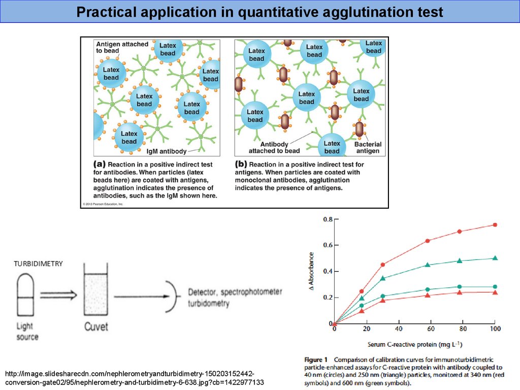
Practical application in quantitative agglutination testhttp://image.slidesharecdn.com/nephlerometryandturbidimetry-150203152442conversion-gate02/95/nephlerometry-and-turbidimetry-6-638.jpg?cb=1422977133
45.
Thank you!Darya Orlova, Ph.D.
Stanford University School of Medicine
Genetics Department
Beckman Building, Room B013
279 Campus Drive, Stanford, CA 94305
orlova@stanford.edu
46.
[2] Moskalensky et al., 2015[3] Xavier et al., 1998
[4] Xavier et al., 1999
I5] Ito et al., 1995
[6] Raman et al., 1992
[7] Nekrasov VM et al., 2014
[8] Ibrahim, M., et al., 1998.
[9] Wibbenmeyer et al., 1999
[10] Sheriff et al., 1987
[11] Chacko et al., 1996
[12] Kam-Morgan et al., 1993
[13] Novotny, 1991
[14] Padlan et al., 1989
[15] Dall’Acqua et al., 1998
[16] Pierce et al., 1999
47.
101 CD8102 103 104
C
D
3
>
CD3
101 102 103 104
C
D
8->
C
D
4->
C
D
4->
101 CD4
102 103 104
101 CD4
102 103 104
A 3-color antibody cocktail (CD4, CD3, CD8) has three 2-D viewing possibilities
C
D
8
>
CD8
101 102 103 104
Number of possible 2-D combinations in n dimensional space:
C
D
3
>
CD3
101 102 103 104
48.
BALB/c PerCB cells (44k/165k events)
49.
BALB/c PerCB cells (44k/165k events)
Shannon entropy score
1.6
1.2
0.8
0.4
0.0
5
10
15
20
25
Dimension pair rank
30
35
40
50.
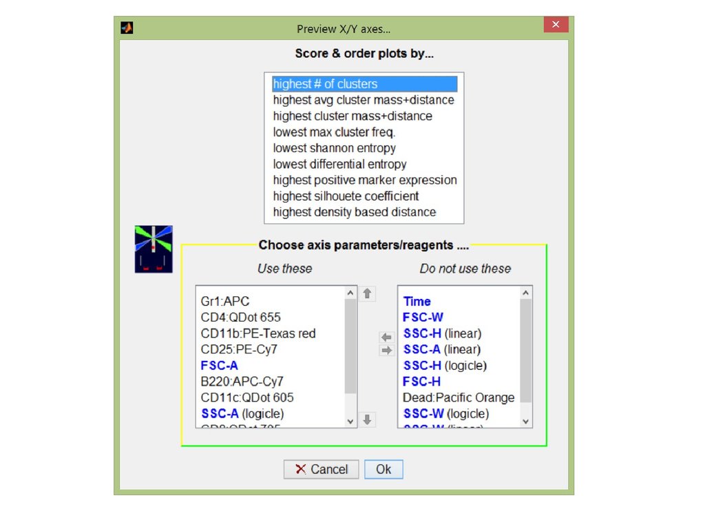
51.
Silhouette coefficient52.
Bb
A
a
1. Calculate silhouette coef. (SC)
For each pair of clusters+their
noise. Calculate % frequency for
each cluster. Find the most
separated (based on SC) pair of
clusters with highest %
frequency (cluster a and b).
2. Assign all other clusters on
this 2D plot either to cluster a
or cluster b based on SC.
3. Now you have only two
clusters A and B (for each
possible 2D plot).
B
A
5. Pick A or B from most highly
ranked 2D plot, project A(or B)
to all possible 2D plots and
proceed recursively with the
same procedure (1-5).
4. Calculate SC between A and B. Calculate %
frequency for A and B. Now you can rank all possible
2D plots based on then SC and % frequency
distribution between A and B. On the first place
should be 2D plot with SC closest to 1 and %
frequency distribution closest to 50/50 between A
and B.
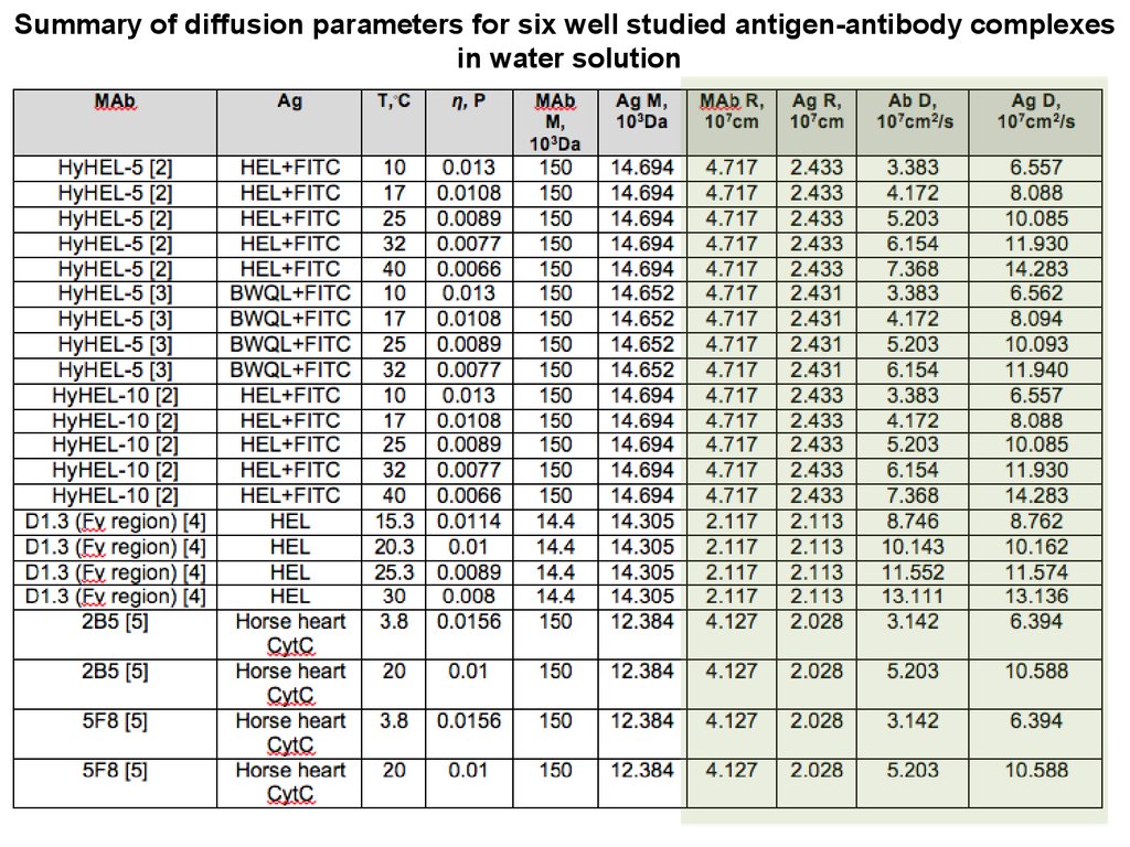
53.
Summary of diffusion parameters for six well studied antigen-antibody complexesin water solution
54.
Agk+, k-
Physics of chemoreception. HC Berg & EM Purcell, Biophys J 20, 93-219 (1977).