Independent Component Analysis

1. Independent Component Analysis

CMPUT 466/551
Nilanjan Ray

2. The Origin of ICA: Factor Analysis

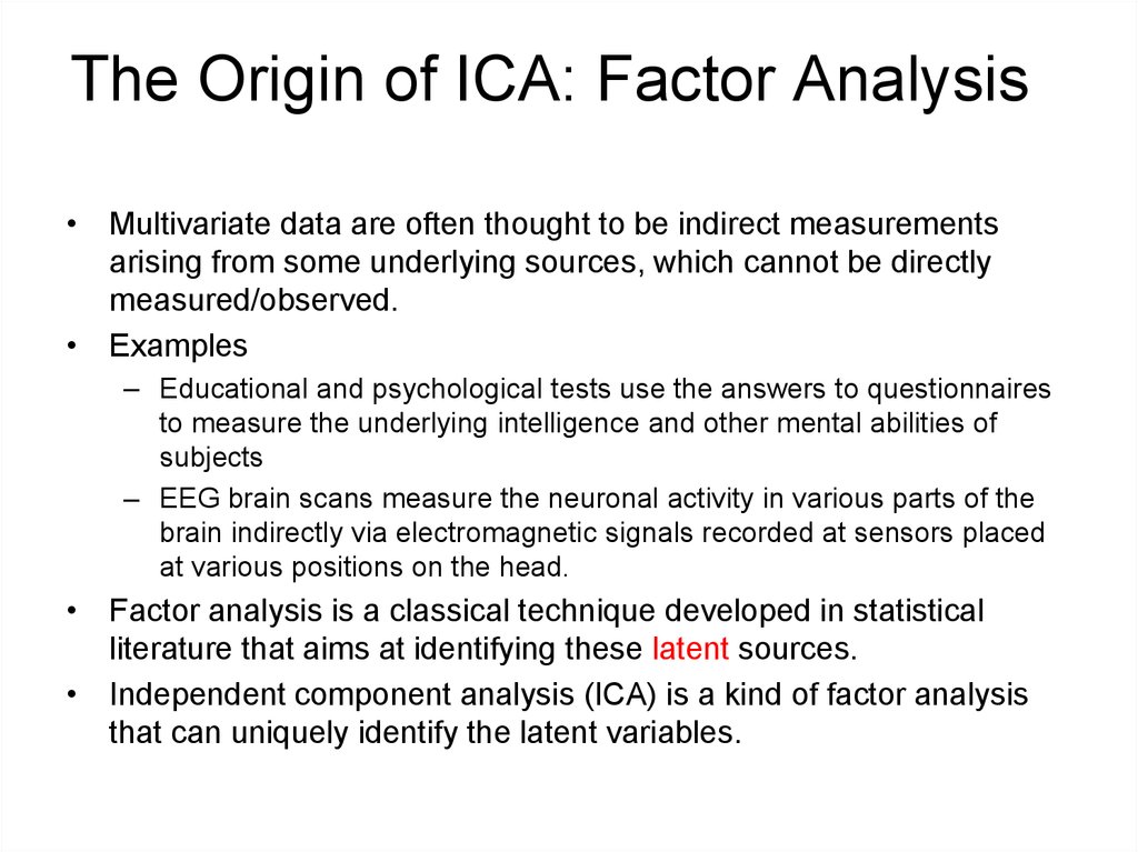
• Multivariate data are often thought to be indirect measurements
arising from some underlying sources, which cannot be directly
measured/observed.
• Examples
– Educational and psychological tests use the answers to questionnaires
to measure the underlying intelligence and other mental abilities of
subjects
– EEG brain scans measure the neuronal activity in various parts of the
brain indirectly via electromagnetic signals recorded at sensors placed
at various positions on the head.
• Factor analysis is a classical technique developed in statistical
literature that aims at identifying these latent sources.
• Independent component analysis (ICA) is a kind of factor analysis
that can uniquely identify the latent variables.

3. Latent Variables and Factor Analysis

X 1 a11S1 a12 S 2 a1 p S p
Latent variable model:
X 2 a21S1 a22 S 2 a2 p S p
or,
X AS
X p a p1S1 a p 2 S 2 a pp S p
Observed variable
Latent components
Mixing matrix
Factor analysis attempts to find out both the mixing coefficients and the
latent components given some instances of observed variables

4. Latent Variables and Factor Analysis…

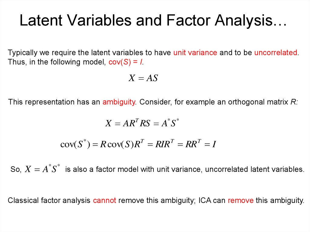
Typically we require the latent variables to have unit variance and to be uncorrelated.
Thus, in the following model, cov(S) = I.
X AS
This representation has an ambiguity. Consider, for example an orthogonal matrix R:
X ART RS A* S *
cov( S * ) R cov( S ) RT RIR T RR T I
So,
X A* S * is also a factor model with unit variance, uncorrelated latent variables.
Classical factor analysis cannot remove this ambiguity; ICA can remove this ambiguity.

5. Classical Factor Analysis

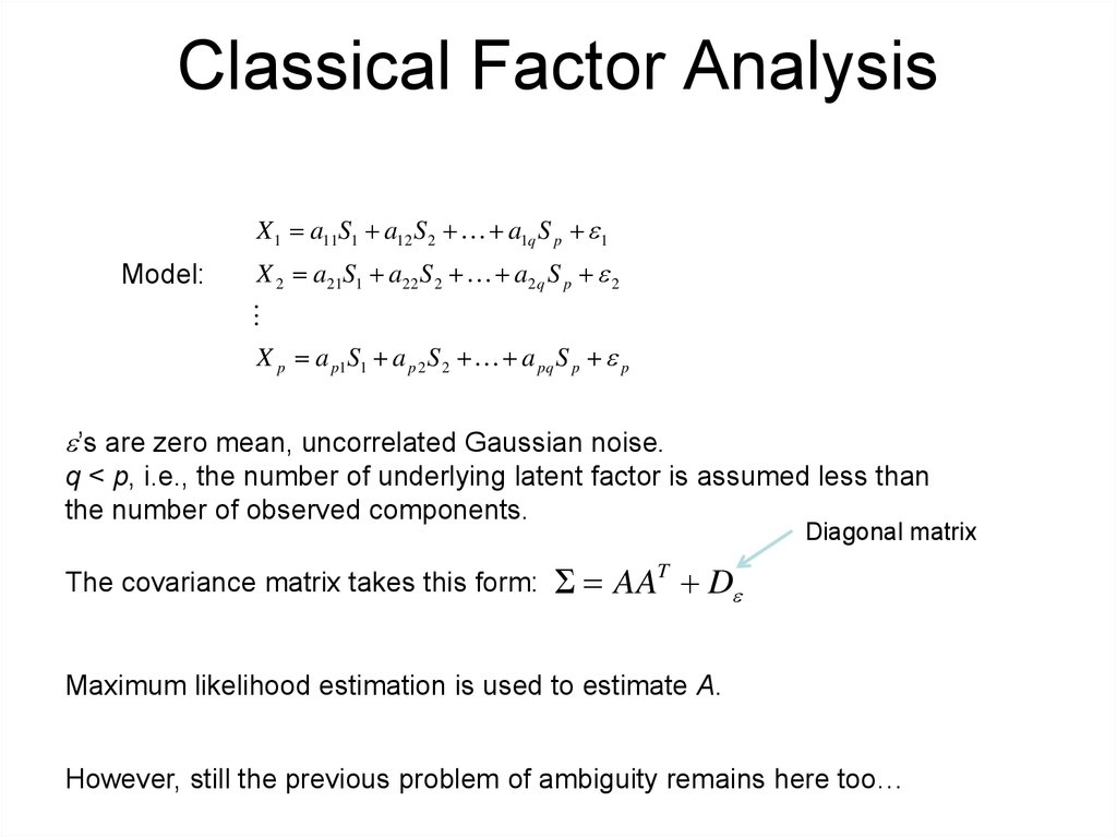
X 1 a11S1 a12 S 2 a1q S p 1
Model:
X 2 a21S1 a22 S 2 a2 q S p 2
X p a p1S1 a p 2 S 2 a pq S p p
’s are zero mean, uncorrelated Gaussian noise.
q < p, i.e., the number of underlying latent factor is assumed less than
the number of observed components.
Diagonal matrix
The covariance matrix takes this form:
AAT D
Maximum likelihood estimation is used to estimate A.
However, still the previous problem of ambiguity remains here too…

6. Independent Component Analysis

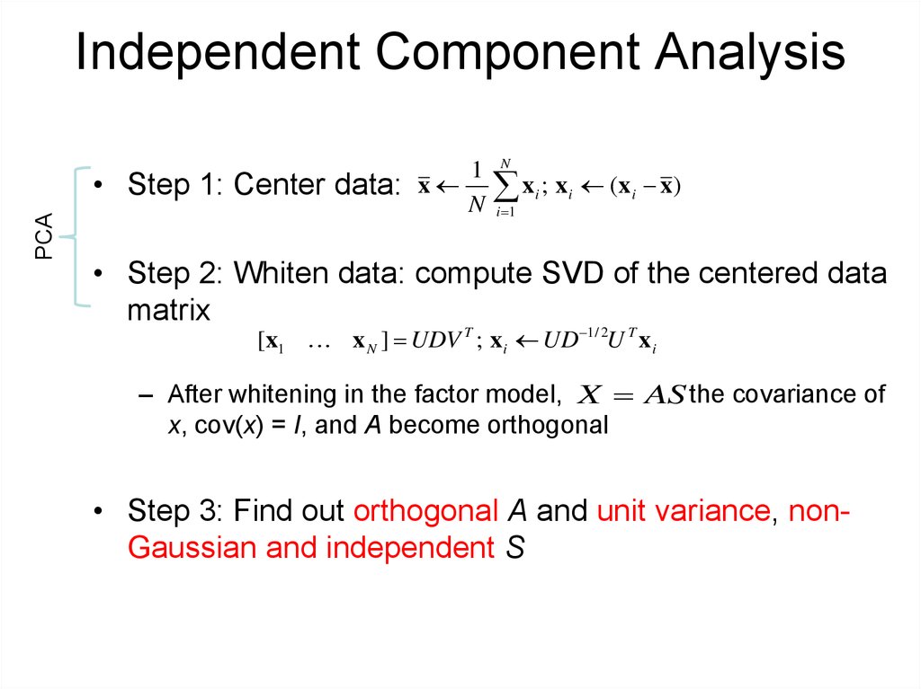
PCA
• Step 1: Center data:
1
x
N
N
x ; x
i 1
i
i
(x i x)
• Step 2: Whiten data: compute SVD of the centered data
matrix
[x1 x N ] UDV T ; x i UD 1/ 2U T x i
– After whitening in the factor model, X AS the covariance of
x, cov(x) = I, and A become orthogonal
• Step 3: Find out orthogonal A and unit variance, nonGaussian and independent S

7. Example: PCA and ICA

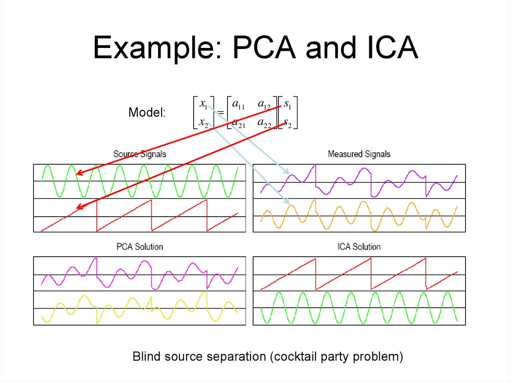
Model:
x1 a11 a12 s1
x a
2 21 a22 s2
Blind source separation (cocktail party problem)

8. PCA vs. ICA

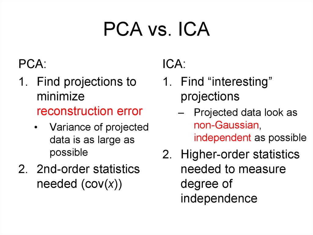
PCA:
1. Find projections to
minimize
reconstruction error
Variance of projected
data is as large as
possible
2. 2nd-order statistics
needed (cov(x))
ICA:
1. Find “interesting”
projections
– Projected data look as
non-Gaussian,
independent as possible
2. Higher-order statistics
needed to measure
degree of
independence

9. Computing ICA

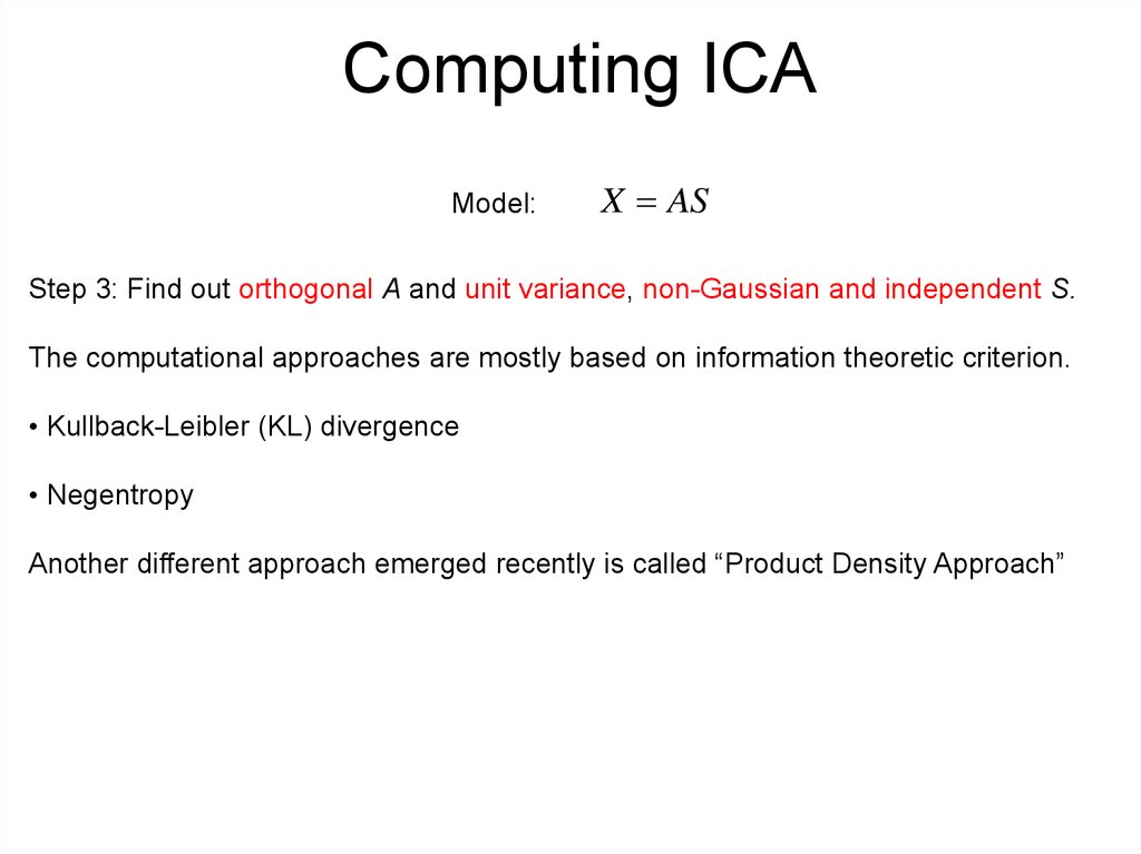
Model:
X AS
Step 3: Find out orthogonal A and unit variance, non-Gaussian and independent S.
The computational approaches are mostly based on information theoretic criterion.
• Kullback-Leibler (KL) divergence
• Negentropy
Another different approach emerged recently is called “Product Density Approach”

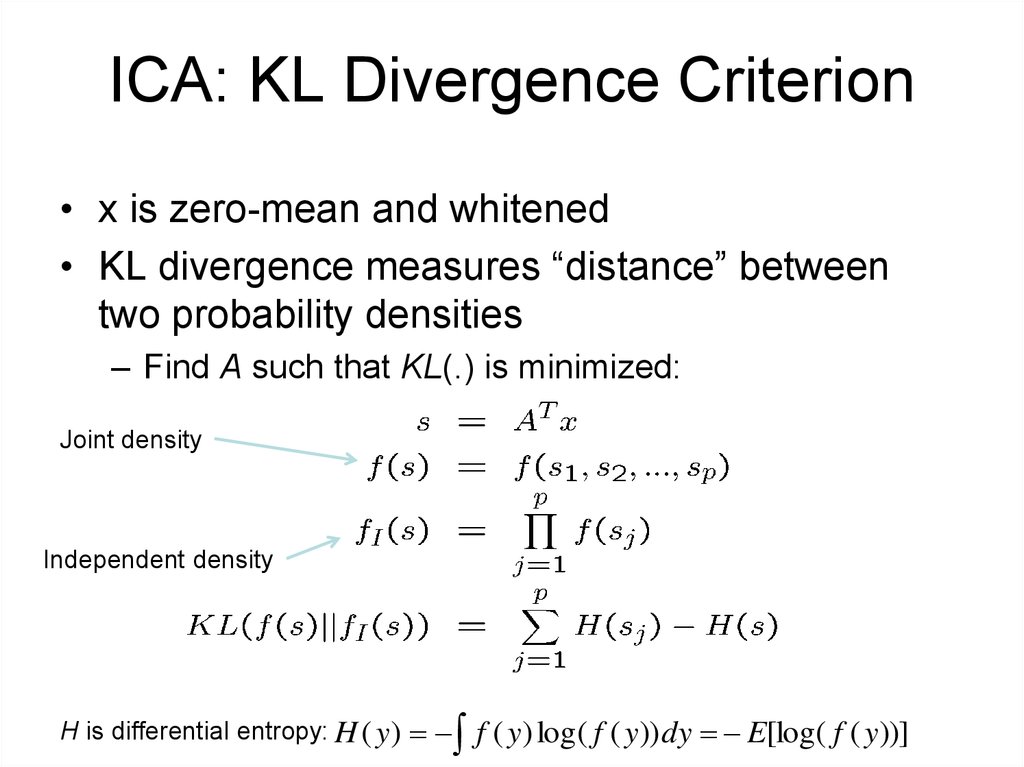
10. ICA: KL Divergence Criterion

• x is zero-mean and whitened
• KL divergence measures “distance” between
two probability densities
– Find A such that KL(.) is minimized:
Joint density
Independent density
H is differential entropy: H ( y )
f ( y ) log( f ( y )) dy E[log( f ( y ))]

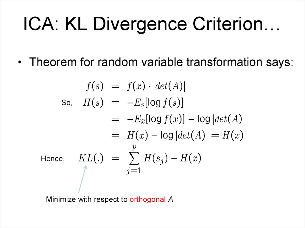
11. ICA: KL Divergence Criterion…

• Theorem for random variable transformation says:
So,
Hence,
Minimize with respect to orthogonal A

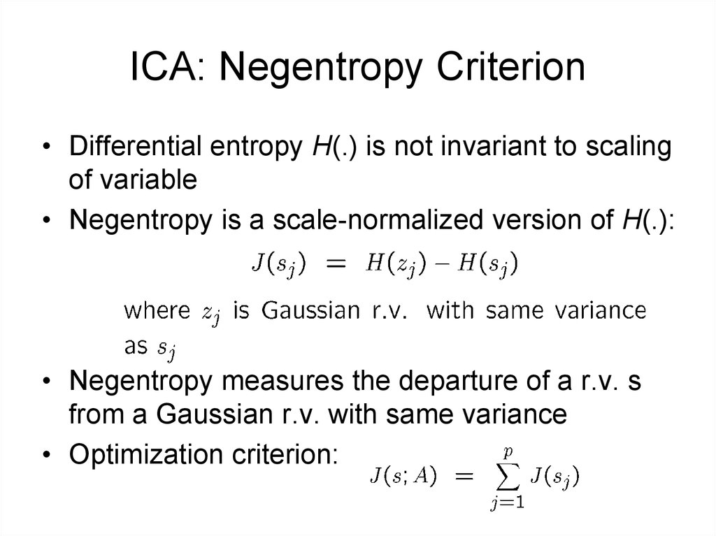
12. ICA: Negentropy Criterion

• Differential entropy H(.) is not invariant to scaling
of variable
• Negentropy is a scale-normalized version of H(.):
• Negentropy measures the departure of a r.v. s
from a Gaussian r.v. with same variance
• Optimization criterion:

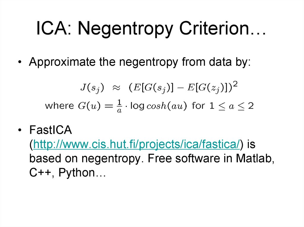
13. ICA: Negentropy Criterion…

• Approximate the negentropy from data by:
• FastICA
(http://www.cis.hut.fi/projects/ica/fastica/) is
based on negentropy. Free software in Matlab,
C++, Python…

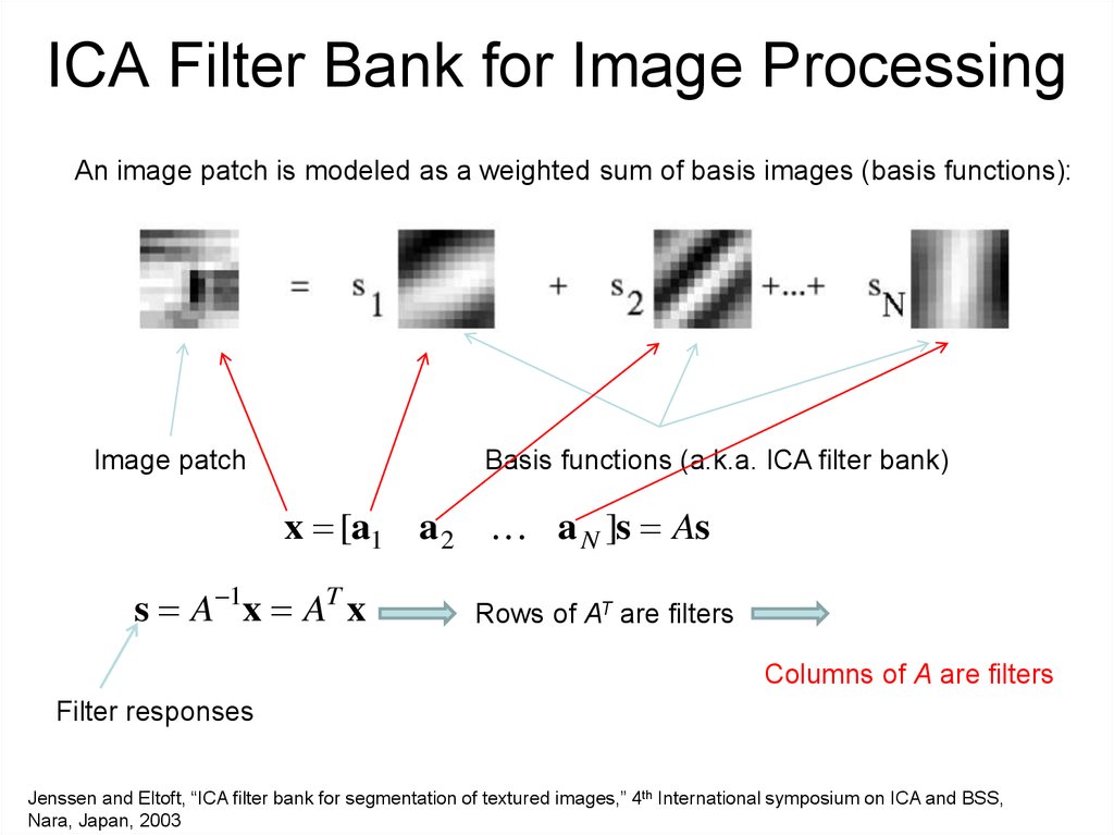
14. ICA Filter Bank for Image Processing

An image patch is modeled as a weighted sum of basis images (basis functions):
Image patch
Basis functions (a.k.a. ICA filter bank)
x [a1 a 2 a N ]s As
s A 1x AT x
Rows of AT are filters
Columns of A are filters
Filter responses
Jenssen and Eltoft, “ICA filter bank for segmentation of textured images,” 4th International symposium on ICA and BSS,
Nara, Japan, 2003

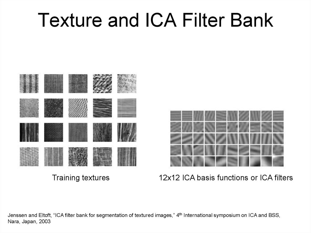
15. Texture and ICA Filter Bank

Training textures
12x12 ICA basis functions or ICA filters
Jenssen and Eltoft, “ICA filter bank for segmentation of textured images,” 4th International symposium on ICA and BSS,
Nara, Japan, 2003

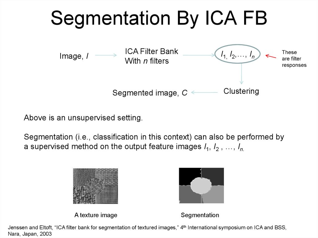
16. Segmentation By ICA FB

ICA Filter Bank
With n filters
Image, I
I1, I2,…, In
Segmented image, C
These
are filter
responses
Clustering
Above is an unsupervised setting.
Segmentation (i.e., classification in this context) can also be performed by
a supervised method on the output feature images I1, I2 , …, In.
A texture image
Segmentation
Jenssen and Eltoft, “ICA filter bank for segmentation of textured images,” 4th International symposium on ICA and BSS,
Nara, Japan, 2003

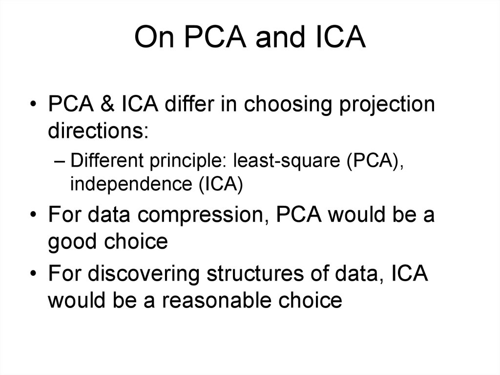
17. On PCA and ICA

• PCA & ICA differ in choosing projection
directions:
– Different principle: least-square (PCA),
independence (ICA)
• For data compression, PCA would be a
good choice
• For discovering structures of data, ICA
would be a reasonable choice