


")


")
")


")


")


 software
Similar presentations:

")


 to create analysis algorithms (open source)")


M/EEG source analysis
1.
M/EEG source analysisRik Henson
MRC CBU, Cambridge
(with thanks to Christophe Phillips, Jeremie Mattout, Gareth
Barnes, Jean Daunizeau, Stefan Kiebel and Karl Friston)
2. Overview
1. Forward Models for M/EEG2. Variational Bayesian Dipole Estimation (ECD)
3. Empirical Bayesian Distributed Estimation
4. Multimodal integration
3. Overview
1. Forward Models for M/EEG2. Variational Bayesian Dipole Estimation (ECD)
3. Empirical Bayesian Distributed Estimation
4. Multimodal integration
4. Bayesian Perspective
Forward Problemm Model
p (Y | , m)
Likelihood
Posterior
Parameters
p ( | Y , m)
p ( | m)
Prior
Evidence
p(Y | m)
Inverse Problem
Y
Data
5. Forward Problem: Physics
Current density:j Orientation
r Location
Likelihood
Y f ( j,r )
Quasi-static
Maxwell’s Equations:
Kirkoff’s law:
j 0
Electrical potential
E
E
E 0
B 0
B j
Y
Y B
(EEG)
(MEG)
6. Forward Problem: Physics
j OrientationLikelihood
Y f ( j,r )
r Location
f
depends on:
location (orientation) of sensors
geometry of head
conductivity of head
(source space)
Can have analytic or numerical form…
7. Forward Problem: Head Models
Concentric Spheres:Pros:
Analytic; Fast to compute
Cons: Head not spherical;
Conductivity not homogeneous
Boundary (or Finite) Element Models:
Pros:
Realistic geometry
Homogeneous conductivity
within boundaries
Cons: Numeric; Slow
Approximation Errors
Other approaches (for MEG): Fit local spheres to each sensor;
Single shell, spherical approx (Nolte)
8. Forward Problem: Meshes
3 important surfaces for BEMs are those with large changes in conductivity:Scalp (skin-air boundary)
Outer Skull (bone-skin boundary)
Inner Skull (CSF-bone boundary)
(Represented as tessellated triangular meshes)
Extracting these surfaces from an MRI is difficult, eg,
because CSF-bone T1-contrast is poor (use PD?)…
A fourth important surface (for some solutions) is:
Cortex (WM-GM boundary)
Extracting this surface from an MRI is very difficult
because so convoluted (though FreeSurfer)…
9. Forward Problem: Canonical Meshes
Rather than extract surfaces from individuals MRIs, why not warp Templatesurfaces from an MNI brain based on spatial (inverse) normalisation?
Henson et al (2009), Neuroimage
10. Recap: (Spatial Normalisation)
fMRI time-seriesAnatomical MRI
Template
Smoothed
Estimate
Spatial Norm
Motion Correct
Smooth
Coregister
m11
m21
m31
0
m12
m22
m32
0
m13
m23
m33
0
Spatially
normalised
m14
m24
m34
1
Deformation
11. Forward Problem: Canonical Meshes
Rather than extract surfaces from individuals MRIs, why not warp Templatesurfaces from an MNI brain based on spatial (inverse) normalisation?
Mattout et al (2007), Comp Int & Neuro
Individual
Canonical
(Inverse-Normalised)
Template
“Canonical”
(Also provides a 1-to-1 mapping across subjects, so source solutions can
be written directly to MNI space, and group-inversion applied; see later)
Given that surfaces are part of the forward model (m), can use the model
evidence p (Y | m) to determine whether Canonical Meshes are sufficient
Henson et al (2009), Neuroimage
12. Forward Problem: ECD vs Distributed
j Orientationr Location
Likelihood
Y f ( j,r )
For small number of Equivalent
Current Dipoles (ECD) anywhere in brain:
f is linear in j but non-linear in r
Y f r j
For (large) number of (Distributed)
dipoles with fixed orientation and location:
f is linear in r
Y F r1 r2 rN J
13. Overview
1. Forward Models for M/EEG2. Variational Bayesian Dipole Estimation (ECD)
3. Empirical Bayesian Distributed Estimation
4. Multimodal integration
14. Inverse Problem: VB-ECD
Standard ECD approaches iterate location/orientation (within a brain volume)until fit to sensor data is maximised (i.e, error minimised). But:
1. Local Minima (particularly when multiple dipoles)
2. Question of how many dipoles?
With a Variational Bayesian (VB) framework, priors can be put on the locations
and orientations (and strengths) of dipoles (e.g, symmetry constraints)
j
r
j
Y f r j e
r
Y
p(r , j , r , j , e | m) p(Y | r , j , e , m) p( e | m) p(r | r , m) p( r | m) p( j | j , m) p( j | m)
Kiebel et al (2008), Neuroimage
15. Inverse Problem: VB-ECD
Maximising the (free-energy approximation to the) model evidence p (Y | m)offers a natural answer to question of the number of dipoles
Kiebel et al (2008), Neuroimage
16. Inverse Problem: DCM
Dynamic Causal Modelling (DCM) can be seen as a source localisation(inverse) method that includes temporal constraints on the source activities
David et al (2011), Journal of Neuroscience
17. Overview
1. Forward Models for M/EEG2. Variational Bayesian Dipole Estimation (ECD)
3. Empirical Bayesian Distributed Estimation
4. Multimodal integration
18.
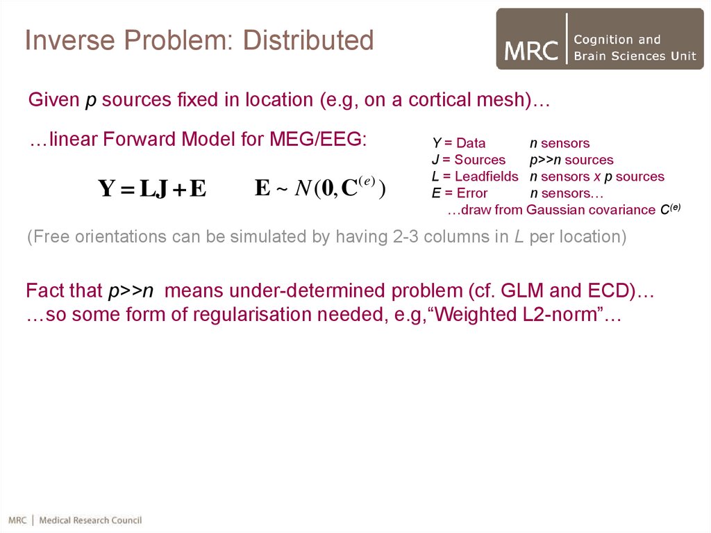
Inverse Problem: DistributedGiven p sources fixed in location (e.g, on a cortical mesh)…
…linear Forward Model for MEG/EEG:
Y = LJ + E
E ~ N (0, C(e ) )
Y = Data
n sensors
J = Sources
p>>n sources
L = Leadfields n sensors x p sources
E = Error
n sensors…
…draw from Gaussian covariance C(e)
(Free orientations can be simulated by having 2-3 columns in L per location)
Fact that p>>n means under-determined problem (cf. GLM and ECD)…
…so some form of regularisation needed, e.g,“Weighted L2-norm”…
19.
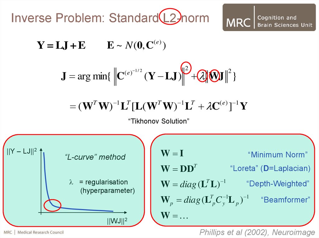
Inverse Problem: Standard L2-normY = LJ + E
E ~ N (0, C(e ) )
J arg min{ C
( e ) 1 / 2
2
(Y LJ ) WJ }
2
( WT W) 1 LT [L( WT W) 1 LT C( e) ] 1 Y
“Tikhonov Solution”
||Y – LJ||2
“L-curve” method
W I
“Minimum Norm”
W DDT
= regularisation
(hyperparameter)
||WJ||2
“Loreta” (D=Laplacian)
W diag (LT L) 1
“Depth-Weighted”
Wp diag (LTp C y 1L p ) 1
“Beamformer”
W
Phillips et al (2002), Neuroimage
20.
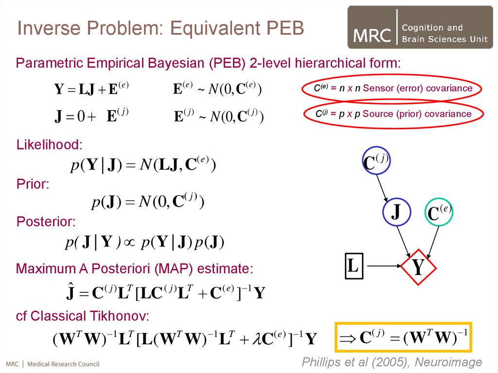
Inverse Problem: Equivalent PEBParametric Empirical Bayesian (PEB) 2-level hierarchical form:
Y LJ Ε(e )
E(e) ~ N (0, C(e) )
C(e) = n x n Sensor (error) covariance
J 0 E( j )
E( j ) ~ N (0, C( j ) )
C(j) = p x p Source (prior) covariance
Likelihood:
p(Y | J ) N (LJ, C( e ) )
Prior:
C( j )
p(J ) N (0, C( j ) )
C (e )
J
Posterior:
p( J | Y ) p(Y | J ) p(J )
L
Maximum A Posteriori (MAP) estimate:
Jˆ C( j ) LT [LC ( j ) LT C( e ) ] 1 Y
Y
cf Classical Tikhonov:
( WT W) 1 LT [L( WT W) 1 LT C(e ) ] 1 Y
C( j ) ( WT W) 1
Phillips et al (2005), Neuroimage
21.
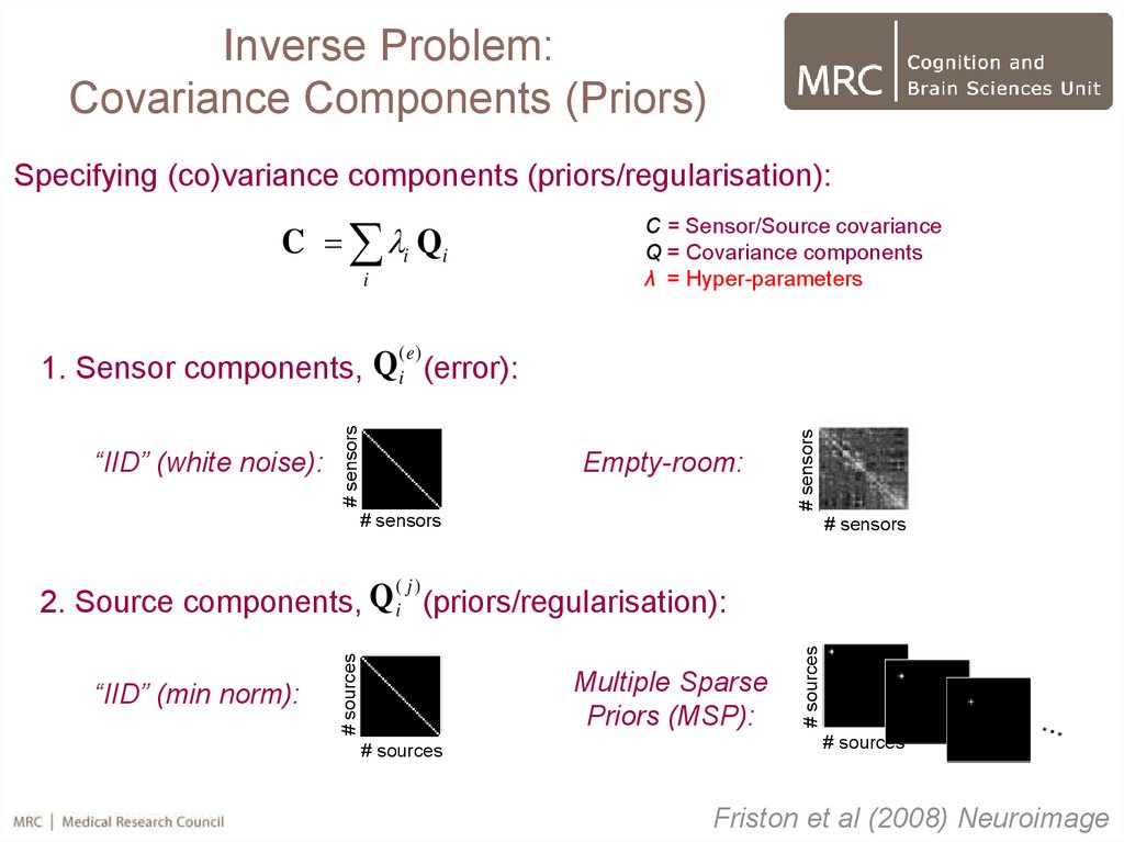
Inverse Problem:Covariance Components (Priors)
Specifying (co)variance components (priors/regularisation):
C i Qi
i
C = Sensor/Source covariance
Q = Covariance components
λ = Hyper-parameters
Empty-room:
# sensors
“IID” (white noise):
# sensors
(e)
1. Sensor components, Qi (error):
# sensors
# sensors
Multiple Sparse
Priors (MSP):
# sources
# sources
“IID” (min norm):
# sources
( j)
Q
2. Source components, i (priors/regularisation):
# sources
Friston et al (2008) Neuroimage
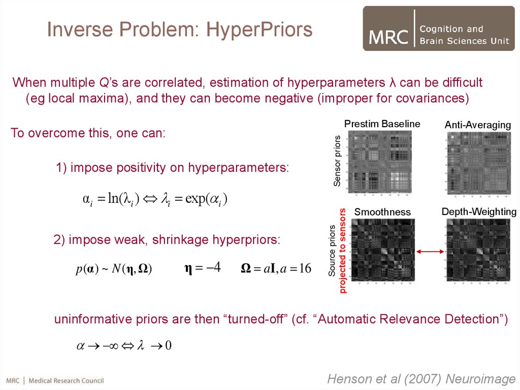
22.
Inverse Problem: HyperPriorsWhen multiple Q’s are correlated, estimation of hyperparameters λ can be difficult
(eg local maxima), and they can become negative (improper for covariances)
αi ln(λi ) i exp( i )
2) impose weak, shrinkage hyperpriors:
p(α ) ~ N ( η, Ω)
η 4
Ω aI, a 16
Anti-Averaging
Smoothness
Depth-Weighting
Sensor priors
1) impose positivity on hyperparameters:
Prestim Baseline
Source priors
projected to sensors
To overcome this, one can:
uninformative priors are then “turned-off” (cf. “Automatic Relevance Detection”)
0
Henson et al (2007) Neuroimage
23.
Inverse Problem: HyperPriorsWhen multiple Q’s are correlated, estimation of hyperparameters λ can be difficult
(eg local maxima), and they can become negative (improper for covariances)
To overcome this, one can:
1) impose positivity on hyperparameters:
αi ln(λi ) i exp( i )
2) impose weak, shrinkage hyperpriors:
p(α ) ~ N ( η, Ω)
η 4
Ω aI, a 16
uninformative priors are then “turned-off” (cf. “Automatic Relevance Detection”)
0
Henson et al (2007) Neuroimage
24.
Inverse Problem: Full (DAG) modelSource and sensor space
η, Ω
Q1( j ) Q (2 j )
...
Q1( e ) Q (2e )
i( e )
i( j )
C( j )
Fixed
...
C( e )
Ε
J
Variable
Data
L
Y
Friston et al (2008) Neuroimage
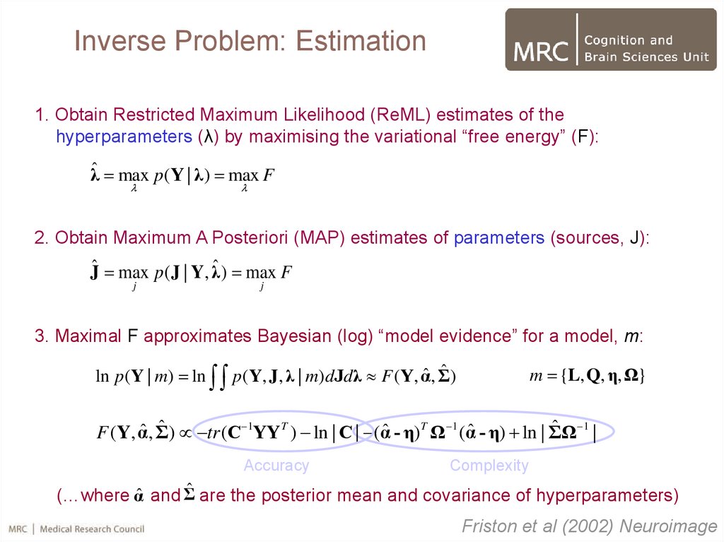
25.
Inverse Problem: Estimation1. Obtain Restricted Maximum Likelihood (ReML) estimates of the
hyperparameters (λ) by maximising the variational “free energy” (F):
λˆ max p(Y | λ ) max F
2. Obtain Maximum A Posteriori (MAP) estimates of parameters (sources, J):
Jˆ max p (J | Y, λˆ ) max F
j
j
3. Maximal F approximates Bayesian (log) “model evidence” for a model, m:
ˆ)
ln p(Y | m) ln p( Y, J, λ | m) dJdλ F ( Y, αˆ , Σ
m {L, Q, η, Ω}
ˆ ) tr (C 1YYT ) ln | C | (αˆ - η)T Ω 1 (αˆ - η) ln | ΣΩ
ˆ 1 |
F (Y, αˆ , Σ
Accuracy
Complexity
(…where α̂ and Σ̂ are the posterior mean and covariance of hyperparameters)
Friston et al (2002) Neuroimage
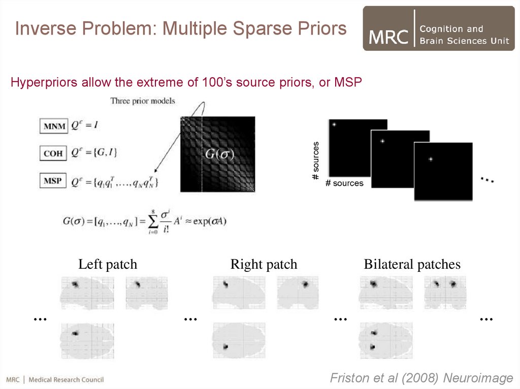
26.
Inverse Problem: Multiple Sparse Priors# sources
Hyperpriors allow the extreme of 100’s source priors, or MSP
# sources
Left patch
…
Right patch
…
Q(2)j
Bilateral patches
…
Q(2)j+1
…
Q(2)j+2
Friston et al (2008) Neuroimage
27.
Inverse Problem: Multiple Sparse PriorsHyperpriors allow the extreme of 100’s source priors, or MSP
Friston et al (2008) Neuroimage
28.
Inverse Problem: PEB SummarySummary:
Automatically “regularises” in principled fashion…
…allows for multiple constraints (priors)…
…to the extent that multiple (100’s) of sparse priors possible (MSP)…
…(or multiple error components or multiple fMRI priors)…
…furnishes estimates of model evidence, so can compare constraints
29. Overview
1. Forward Models for M/EEG2. Variational Bayesian Dipole Estimation (ECD)
3. Empirical Bayesian Distributed Estimation
4. Multi-modal and multi-subject integration
30. Multi-subject Integration (Group Inversion)
Specifying (co)variance components (priors/regularisation):C i Qi
i
C = Sensor/Source covariance
Q = Covariance components
λ = Hyper-parameters
Empty-room:
# sensors
“IID” (white noise):
# sensors
(e)
1. Sensor components, Qi (error):
# sensors
# sensors
Multiple Sparse
Priors (MSP):
# sources
# sources
“IID” (min norm):
# sources
( j)
Q
2. Source components, i (priors/regularisation):
# sources
Friston et al (2008) Neuroimage
31. Multi-subject Integration (Group Inversion)
Specifying (co)variance components (priors/regularisation):C i Qi
i
C = Sensor/Source covariance
Q = Covariance components
λ = Hyper-parameters
Empty-room:
# sensors
# sensors
“IID” (white noise):
# sensors
(e)
1. Sensor components, Qi (error):
# sensors
# sources
( j)
2. Optimise Multiple Sparse Priors by pooling across subjects Qi
# sources
Litvak & Friston (2008) Neuroimage
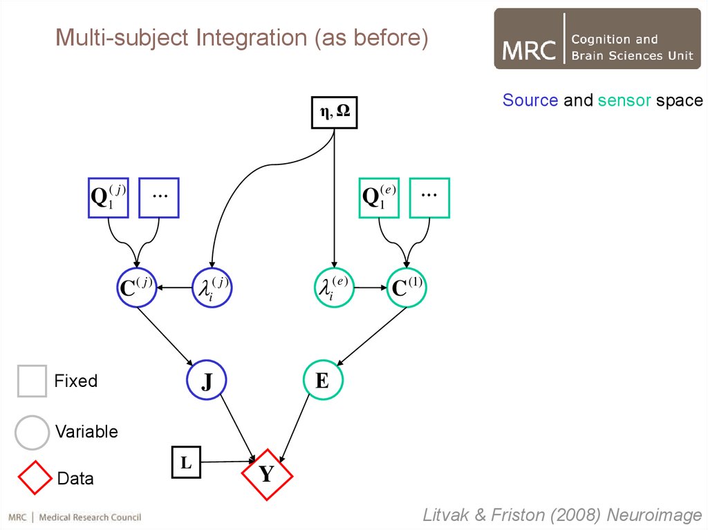
32.
Multi-subject Integration (as before)Source and sensor space
η, Ω
Q1( j )
...
Q1( e )
C( j )
Fixed
i( j )
i( e )
J
Ε
...
C (1)
Variable
Data
L
Y
Litvak & Friston (2008) Neuroimage
33.
Multi-subject IntegrationSource and sensor space
η, Ω
Q1( j )
...
(e)
Q11
λ1( e )
λ ( j)
C( j )
Ε1
J1
Fixed
...
Q (21e )
λ (2e )
C1(1)
...
C (1)
2
Ε2
J2
Variable
Data
L1
Y1
Y2
L2
Litvak & Friston (2008) Neuroimage
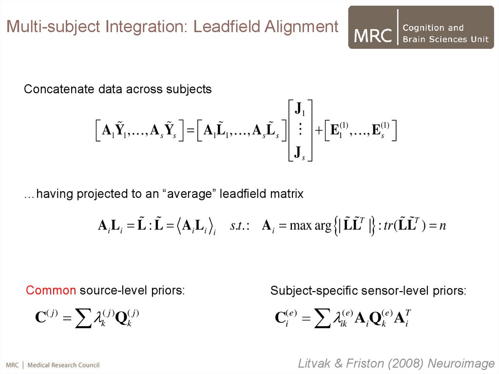
34.
Multi-subject Integration: Leadfield AlignmentConcatenate data across subjects
J1
A1Y1 , , A s Ys A1L1 , , A s L s E1(1) , , E(1)
s
J s
…having projected to an “average” leadfield matrix
A i Li L : L A i Li
Common source-level priors:
C( j ) k( j )Q(k j )
i
s.t.: Ai max arg | LLT | : tr (LLT ) n
Subject-specific sensor-level priors:
Ci(e) ik(e) AiQ(ke) ATi
Litvak & Friston (2008) Neuroimage
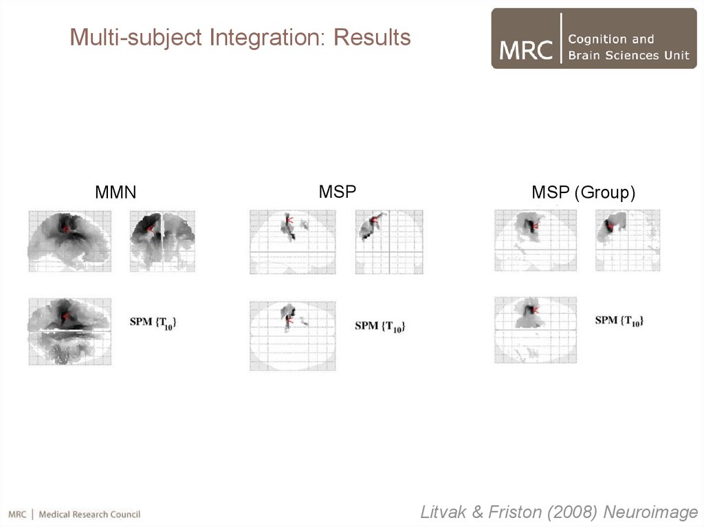
35.
Multi-subject Integration: ResultsMMN
MSP
MSP (Group)
Litvak & Friston (2008) Neuroimage
36. Multi-modal Integration
1. Symmetric integration (fusion) of MEG + EEG2. Asymmetric integration of M/EEG + fMRI
3. Full fusion of M/EEG + fMRI?
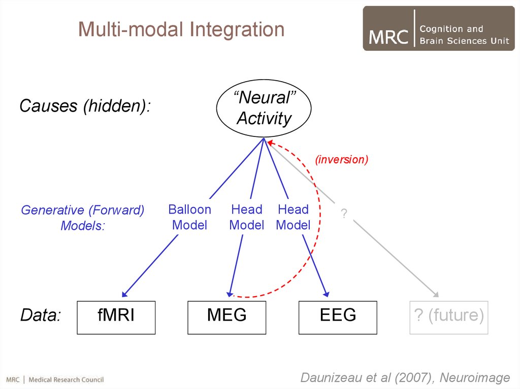
37.
Multi-modal Integration“Neural”
Activity
Causes (hidden):
(inversion)
Generative (Forward)
Models:
Data:
fMRI
Balloon
Model
Head Head
Model Model
MEG
?
EEG
? (future)
Daunizeau et al (2007), Neuroimage
38.
Multi-modal Integration“Neural”
Activity
Causes (hidden):
Generative (Forward)
Models:
Data:
Balloon
Model
fMRI
Head Head
Model Model
MEG
?
EEG
Symmetric
Integration
(Fusion)
? (future)
Asymmetric
Integration
Daunizeau et al (2007), Neuroimage
39. Multi-modal Integration
1. Symmetric integration (fusion) of MEG + EEG2. Asymmetric integration of M/EEG + fMRI
3. Full fusion of M/EEG + fMRI?
40.
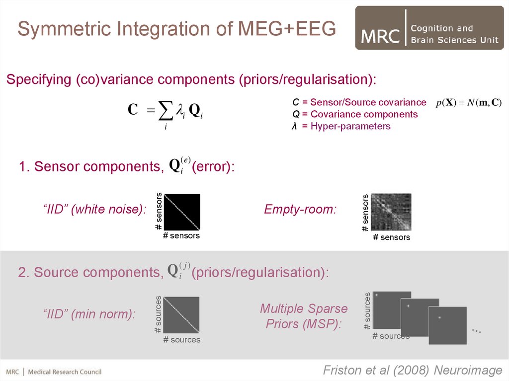
Symmetric Integration of MEG+EEGSpecifying (co)variance components (priors/regularisation):
C i Qi
i
C = Sensor/Source covariance p( X) N (m, C)
Q = Covariance components
λ = Hyper-parameters
Empty-room:
# sensors
“IID” (white noise):
# sensors
(e)
1. Sensor components, Qi (error):
# sensors
# sensors
Multiple Sparse
Priors (MSP):
# sources
# sources
“IID” (min norm):
# sources
( j)
Q
2. Source components, i (priors/regularisation):
# sources
Friston et al (2008) Neuroimage
41.
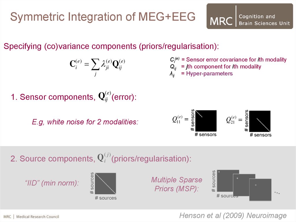
Symmetric Integration of MEG+EEGSpecifying (co)variance components (priors/regularisation):
C Q
(e)
i
(e)
ji
(e)
ij
j
Ci(e) = Sensor error covariance for ith modality
Qij = jth component for ith modality
λij = Hyper-parameters
Q21( e )
# sensors
# sensors
E.g, white noise for 2 modalities:
Q11( e )
# sensors
(e)
1. Sensor components, Qij (error):
# sensors
Multiple Sparse
Priors (MSP):
# sources
# sources
“IID” (min norm):
# sources
( j)
Q
2. Source components, i (priors/regularisation):
# sources
Henson et al (2009) Neuroimage
42.
Single Modality (as before)η, Ω
Qi(2)
...
Q i(1)
i(1)
i(2)
C(2)
...
C (1)
Ε1
J
Fixed
Source and sensor space
Variable
L
Data
Y
Henson et al (2009) Neuroimage
43.
Multiple modalitiesη, Ω
Qi(2)
...
Q1i(1)
λ1(1)
λ ( 2)
C(2)
...
Q (1)
2i
λ (1)
2
...
C (1)
2
Ε2
Ε1
J
Fixed
C1(1)
Source and sensor space
Variable
L1
Data
Y1
Y2
L2
Henson et al (2009) Neuroimage
44.
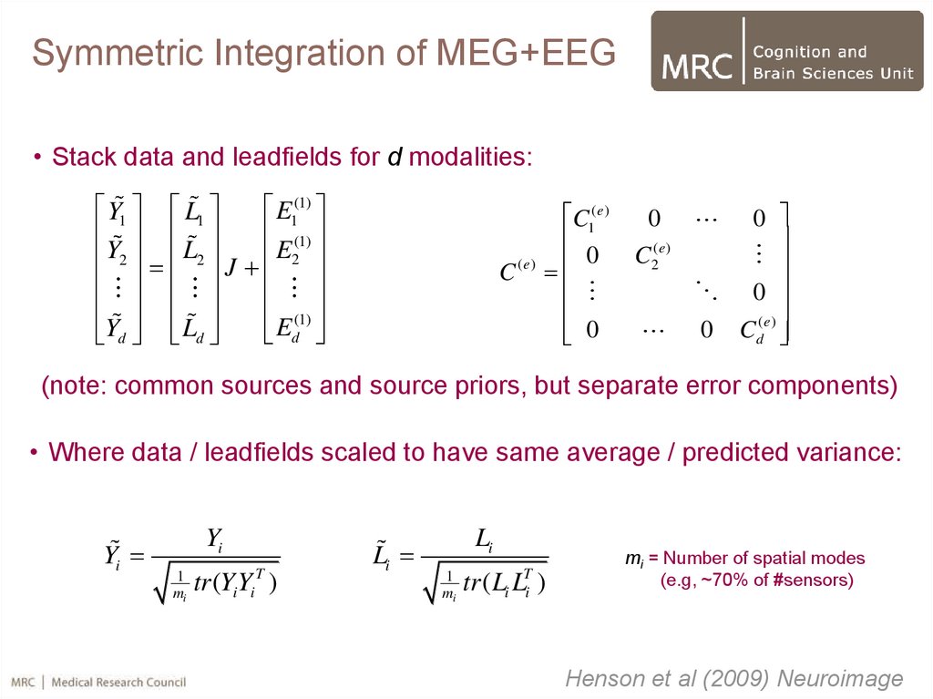
Symmetric Integration of MEG+EEG• Stack data and leadfields for d modalities:
Y1 L1
E1(1)
(1)
Y
L
2 2 J E2
(1)
Y
L
Ed
d d
C (e)
C1( e )
0
0
0 0
C2( e )
0
(e)
0 Cd
(note: common sources and source priors, but separate error components)
• Where data / leadfields scaled to have same average / predicted variance:
Yi
Yi
1
mi
T
tr (YiYi )
Li
Li
1
mi
T
i i
tr ( L L )
mi = Number of spatial modes
(e.g, ~70% of #sensors)
Henson et al (2009) Neuroimage
45.
Symmetric Integration of MEG+EEGERs from 12 subjects for 3 simultaneously-acquired Neuromag sensor-types:
(Planar) Gradiometers
(MEG, 204)
Electrodes
(EEG, 70)
μV
fT
RMS fT/m
Magnetometers
(MEG, 102)
Faces
Scrambled
ms
ms
ms
Faces - Scrambled
150-190ms
Henson et al (2009) Neuroimage
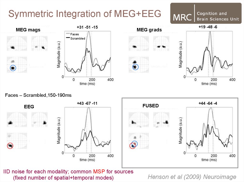
46.
Symmetric Integration of MEG+EEG+31 -51 -15
MEG mags
MEG grads
+19 -48 -6
Faces
Scrambled
Faces – Scrambled,150-190ms
EEG
+43 -67 -11
IID noise for each modality; common MSP for sources
(fixed number of spatial+temporal modes)
FUSED
+44 -64 -4
Henson et al (2009) Neuroimage
47.
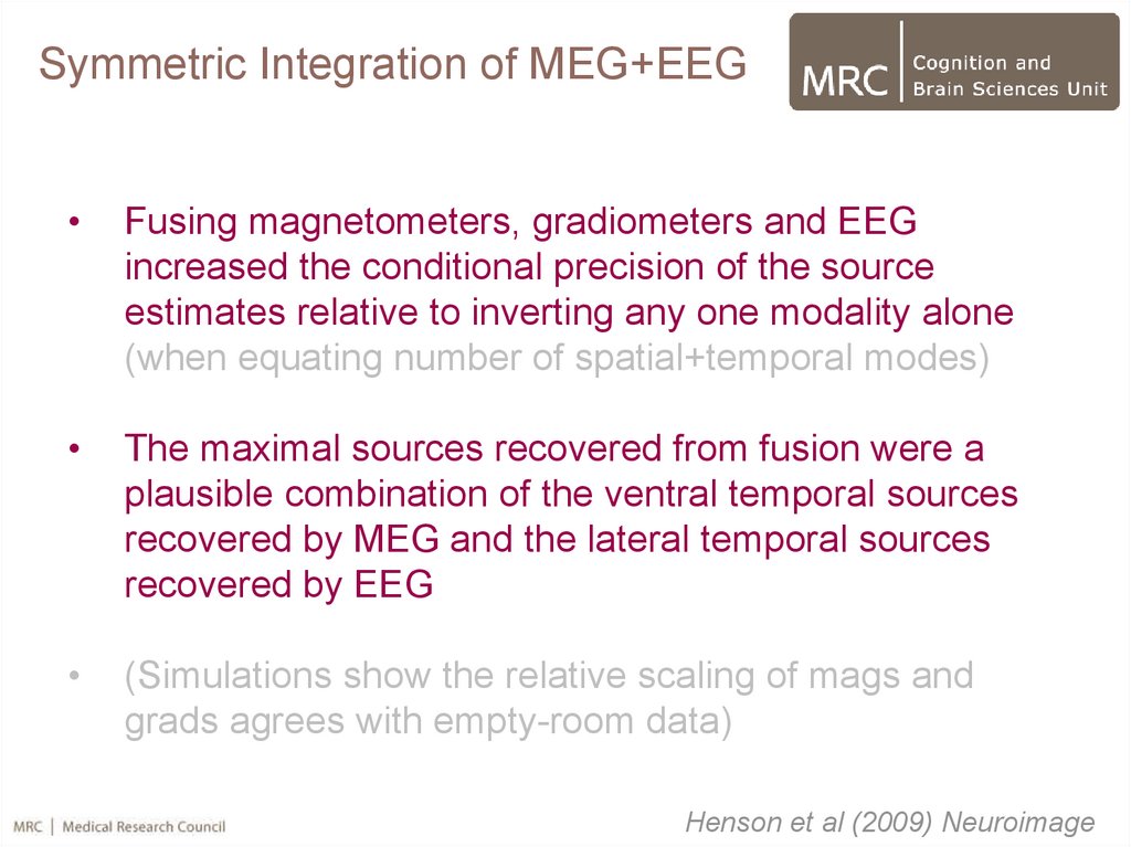
Symmetric Integration of MEG+EEGFusing magnetometers, gradiometers and EEG
increased the conditional precision of the source
estimates relative to inverting any one modality alone
(when equating number of spatial+temporal modes)
The maximal sources recovered from fusion were a
plausible combination of the ventral temporal sources
recovered by MEG and the lateral temporal sources
recovered by EEG
(Simulations show the relative scaling of mags and
grads agrees with empty-room data)
Henson et al (2009) Neuroimage
48. Multi-modal Integration
1. Symmetric integration (fusion) of MEG + EEG2. Asymmetric integration of M/EEG + fMRI
3. Full fusion of M/EEG + fMRI?
49. Asymmetric Integration of M/EEG+fMRI
Specifying (co)variance components (priors/regularisation):C i Qi
i
C = Sensor/Source covariance p( X) N (m, C)
Q = Covariance components
λ = Hyper-parameters
Empty-room:
# sensors
“IID” (white noise):
# sensors
(e)
1. Sensor components, Qi (error):
# sensors
# sensors
Multiple Sparse
Priors (MSP):
# sources
# sources
“IID” (min norm):
# sources
( j)
Q
2. Source components, i (priors/regularisation):
# sources
Friston et al (2008) Neuroimage
50.
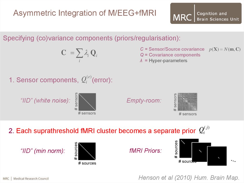
Asymmetric Integration of M/EEG+fMRISpecifying (co)variance components (priors/regularisation):
C i Qi
i
C = Sensor/Source covariance p( X) N (m, C)
Q = Covariance components
λ = Hyper-parameters
Empty-room:
# sensors
“IID” (white noise):
# sensors
(e)
1. Sensor components, Qi (error):
# sensors
# sensors
fMRI Priors:
# sources
# sources
“IID” (min norm):
# sources
( j)
Q
2. Each suprathreshold fMRI cluster becomes a separate prior i
# sources
Henson et al (2010) Hum. Brain Map.
51.
Asymmetric Integration of M/EEG+fMRISource and sensor space
η, Ω
Q1( j ) Q (2 j )
...
Q1( e ) Q (2e )
i( e )
i( j )
C( j )
Fixed
...
C (1)
Ε
J
Variable
Data
L
Y
Friston et al (2008) Neuroimage
52.
Asymmetric Integration of M/EEG+fMRIη, Ω
Y
fMRI
Q1( j ) Q (2 j )
Source and sensor space
...
Q1( e ) Q (2e )
i( e )
i( j )
C( j )
Fixed
...
C (1)
Ε
J
Variable
Data
L
Y
M / EEG
Henson et al (2010) Hum. Brain Map.
53.
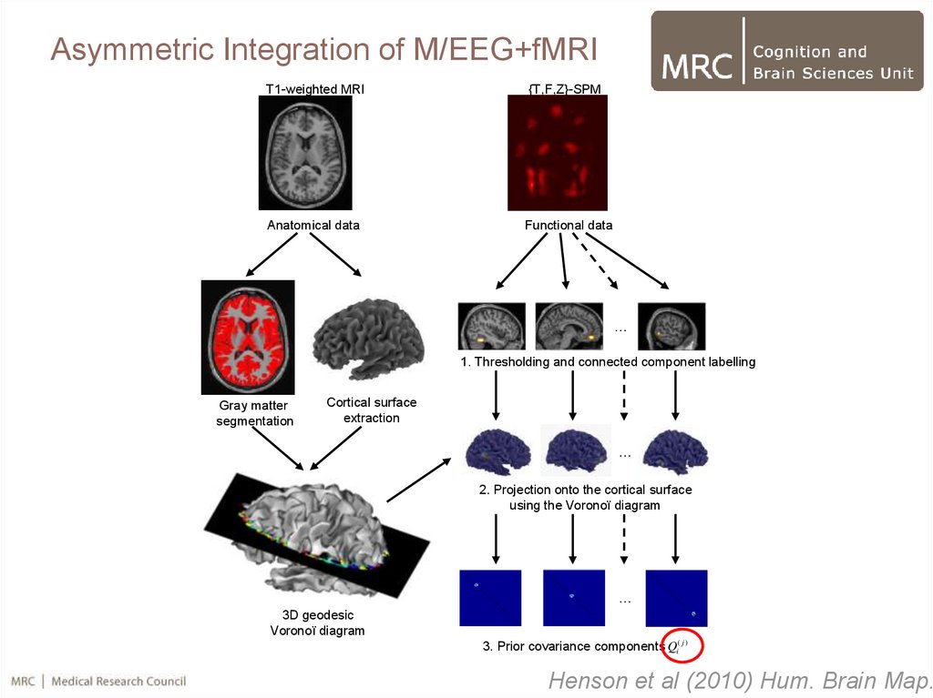
Asymmetric Integration of M/EEG+fMRIT1-weighted MRI
Anatomical data
{T,F,Z}-SPM
Functional data
…
1. Thresholding and connected component labelling
Gray matter
segmentation
Cortical surface
extraction
…
2. Projection onto the cortical surface
using the Voronoï diagram
…
3D geodesic
Voronoï diagram
3. Prior covariance components Qi( j )
Henson et al (2010) Hum. Brain Map.
54.
Asymmetric Integration of M/EEG+fMRI1
2
4
5
SPM{F} for faces versus
scrambled faces,
15 voxels, p<.05 FWE
3
5 clusters from SPM of fMRI data from separate group of (18)
subjects in MNI space
Henson et al (2010) Hum. Brain Map.
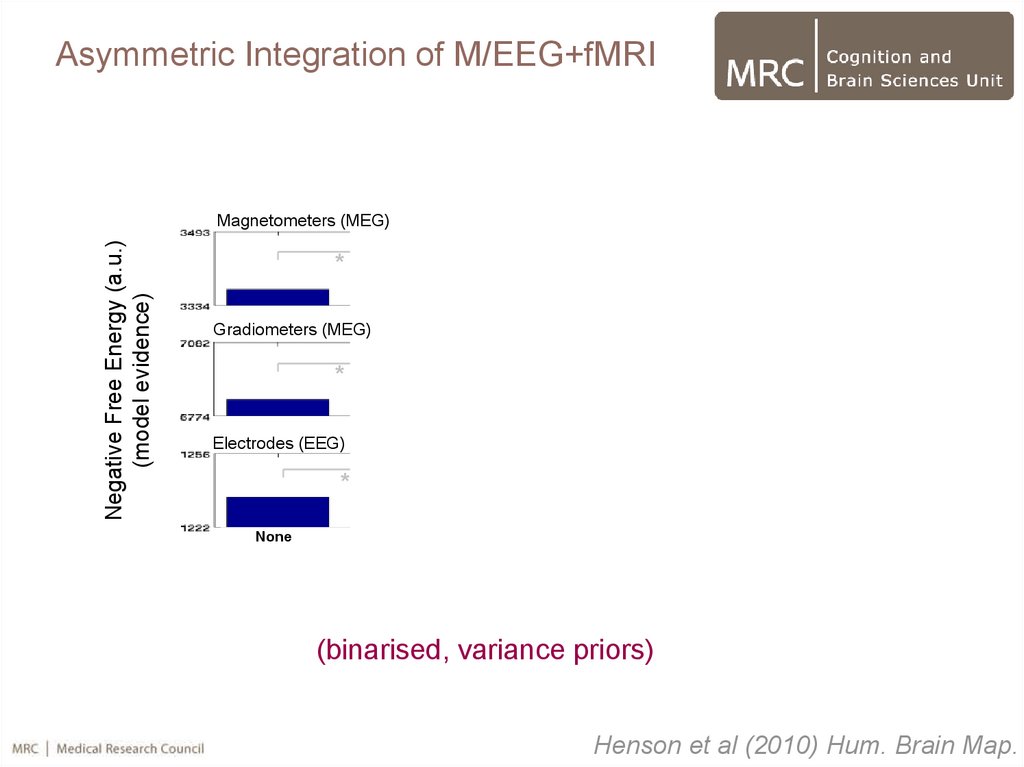
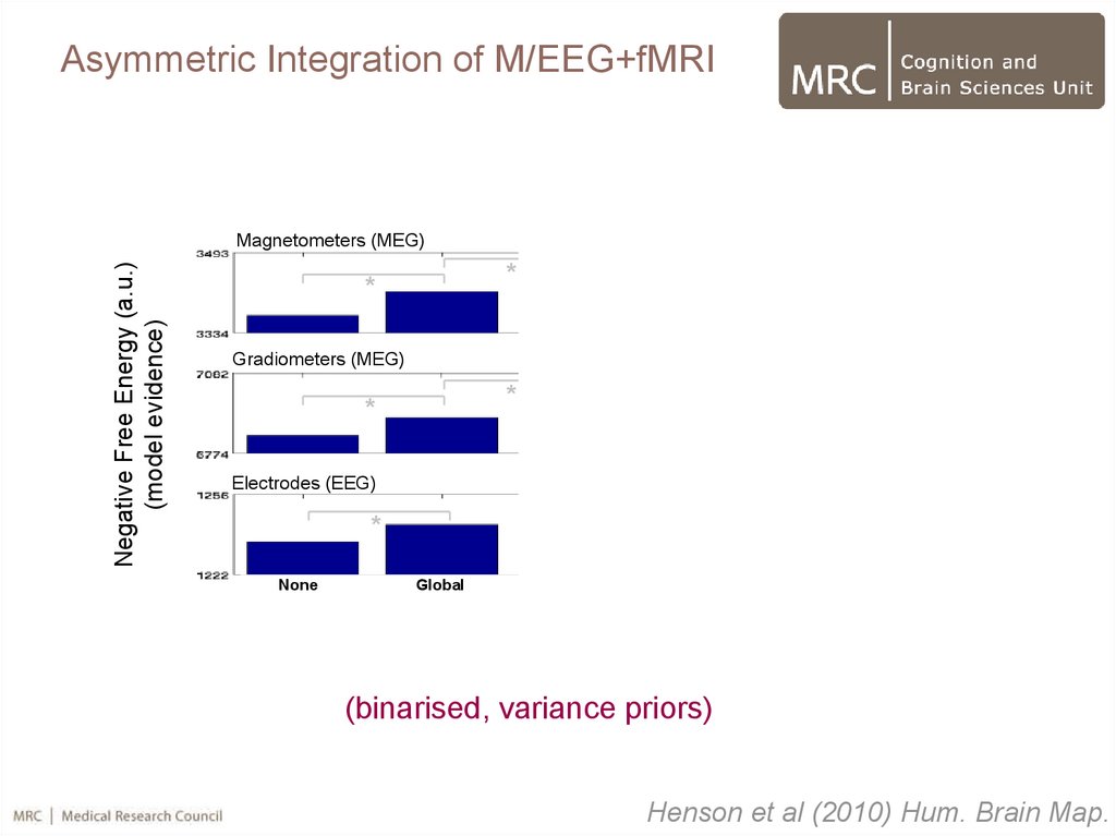
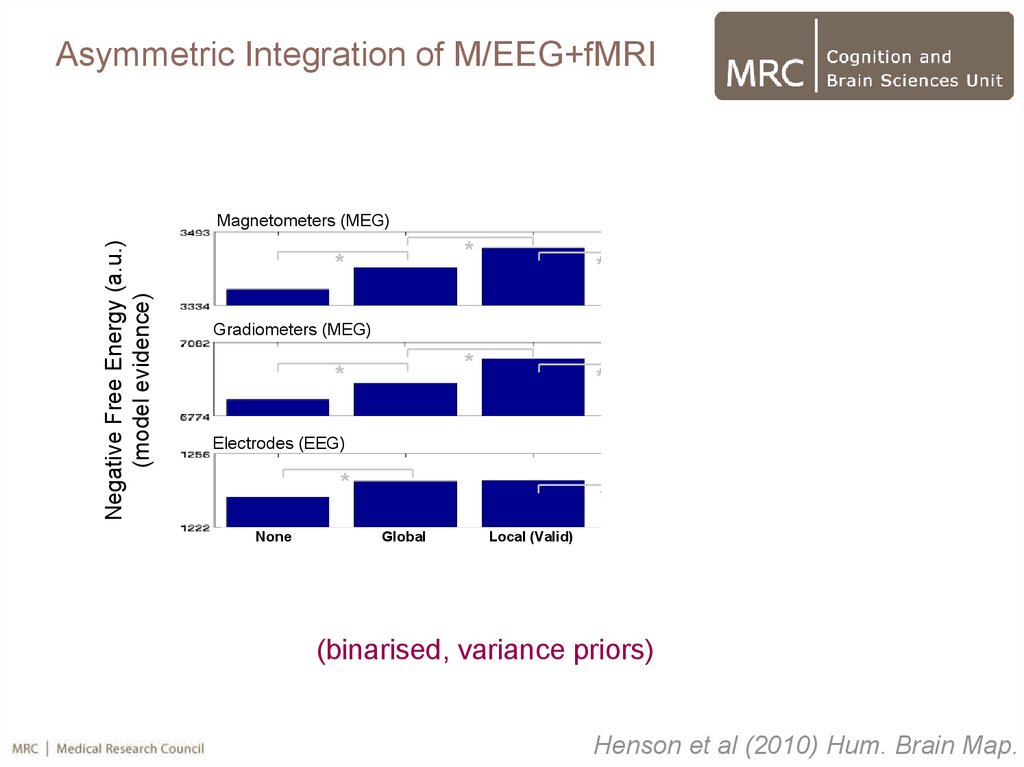
55.
Asymmetric Integration of M/EEG+fMRINegative Free Energy (a.u.)
(model evidence)
Magnetometers (MEG)
*
*
*
*
Gradiometers (MEG)
*
*
*
*
Electrodes (EEG)
*
None
*
*
Global
Local (Valid)
Local (Invalid)
Valid+Invalid
(binarised, variance priors)
Henson et al (2010) Hum. Brain Map.
56.
Asymmetric Integration of M/EEG+fMRINegative Free Energy (a.u.)
(model evidence)
Magnetometers (MEG)
*
*
*
*
Gradiometers (MEG)
*
*
*
*
Electrodes (EEG)
*
None
*
*
Global
Local (Valid)
Local (Invalid)
Valid+Invalid
(binarised, variance priors)
Henson et al (2010) Hum. Brain Map.
57.
Asymmetric Integration of M/EEG+fMRINegative Free Energy (a.u.)
(model evidence)
Magnetometers (MEG)
*
*
*
*
Gradiometers (MEG)
*
*
*
*
Electrodes (EEG)
*
None
*
*
Global
Local (Valid)
Local (Invalid)
Valid+Invalid
(binarised, variance priors)
Henson et al (2010) Hum. Brain Map.
58. 3.2 Fusion of MEG+fMRI (Application)
Negative Free Energy (a.u.)(model evidence)
Magnetometers (MEG)
*
*
*
*
Gradiometers (MEG)
*
*
*
*
Electrodes (EEG)
*
None
*
*
Global
Local (Valid)
Local (Invalid)
Valid+Invalid
(binarised, variance priors)
Henson et al (2010) Hum. Brain Map.
59.
Asymmetric Integration of M/EEG+fMRINegative Free Energy (a.u.)
(model evidence)
Magnetometers (MEG)
*
*
*
*
Gradiometers (MEG)
*
*
*
*
Electrodes (EEG)
*
None
*
*
Global
Local (Valid)
Local (Invalid)
Valid+Invalid
(binarised, variance priors)
Henson et al (2010) Hum. Brain Map.
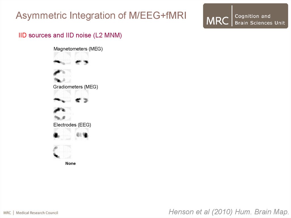
60.
Asymmetric Integration of M/EEG+fMRIIID sources and IID noise (L2 MNM)
Magnetometers (MEG)
Gradiometers (MEG)
Electrodes (EEG)
None
Global
Local (Valid)
Local (Invalid)
Henson et al (2010) Hum. Brain Map.
61.
Asymmetric Integration of M/EEG+fMRIIID sources and IID noise (L2 MNM)
Magnetometers (MEG)
Gradiometers (MEG)
Electrodes (EEG)
None
Global
Local (Valid)
Local (Invalid)
Henson et al (2010) Hum. Brain Map.
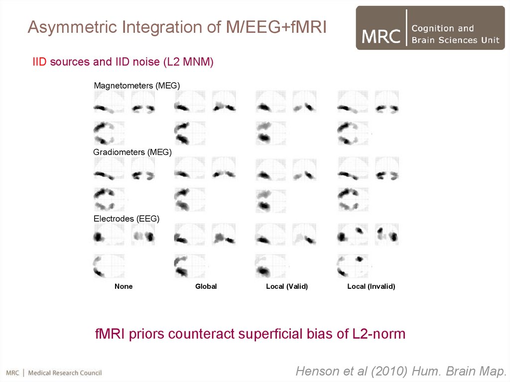
62. 3.2 Fusion of MEG+fMRI (Application)
IID sources and IID noise (L2 MNM)Magnetometers (MEG)
Gradiometers (MEG)
Electrodes (EEG)
None
Global
Local (Valid)
Local (Invalid)
fMRI priors counteract superficial bias of L2-norm
Henson et al (2010) Hum. Brain Map.
63.
Asymmetric Integration of M/EEG+fMRIIID sources and IID noise (L2 MNM)
Magnetometers (MEG)
Gradiometers (MEG)
Electrodes (EEG)
None
Global
Local (Valid)
Local (Invalid)
fMRI priors counteract superficial bias of L2-norm
Henson et al (2010) Hum. Brain Map.
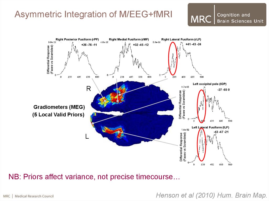
64.
Asymmetric Integration of M/EEG+fMRIDifferential Response
(Faces vs Scrambled)
Right Posterior Fusiform (rPF)
+26 -76 -11
Right Medial Fusiform (rMF)
Right Lateral Fusiform (rLF)
+32 -45 -12
+41 -43 -24
Gradiometers (MEG)
(5 Local Valid Priors)
L
Differential Response
(Faces vs Scrambled)
R
Differential Response
(Faces vs Scrambled)
Left occipital pole (lOP)
-27 -93 0
Left Lateral Fusiform (lLF)
-43 -47 -21
NB: Priors affect variance, not precise timecourse…
Henson et al (2010) Hum. Brain Map.
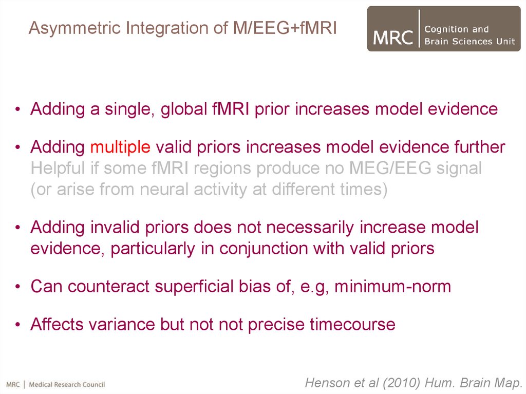
65.
Asymmetric Integration of M/EEG+fMRI• Adding a single, global fMRI prior increases model evidence
• Adding multiple valid priors increases model evidence further
Helpful if some fMRI regions produce no MEG/EEG signal
(or arise from neural activity at different times)
• Adding invalid priors does not necessarily increase model
evidence, particularly in conjunction with valid priors
• Can counteract superficial bias of, e.g, minimum-norm
• Affects variance but not not precise timecourse
Henson et al (2010) Hum. Brain Map.
66. Multi-modal Integration
1. Symmetric integration (fusion) of MEG + EEG2. Asymmetric integration of M/EEG + fMRI
3. Full fusion of M/EEG + fMRI?
67. Fusion of fMRI and MEG/EEG?
“Neural”Activity
Causes (hidden):
Fusion of fMRI +
MEG/EEG?
Data:
fMRI
Balloon
Model
Head Head
Model Model
MEG
?
EEG
? (future)
Henson (2010) Biomag
68.
Fusion of fMRI and MEG/EEG?η, Ω
Qi(2)
...
Q i(1)
i(2)
C(2)
Fixed
Source and sensor space
i(1)
...
C (1)
Ε1
J
Variable
Data
Y
L1
M / EEG
Henson Et Al (2011) Frontiers
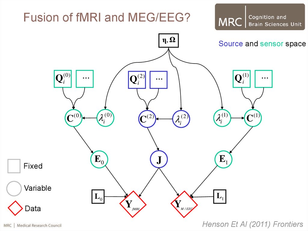
69.
Fusion of fMRI and MEG/EEG?η, Ω
Qi(0)
C(0)
Fixed
...
Qi(2)
i(0)
...
Q i(1)
i(2)
C(2)
Ε0
Source and sensor space
i(1)
...
C (1)
Ε1
J
Variable
L0
Data
Y
fMRI
Y
L1
M / EEG
Henson Et Al (2011) Frontiers
70.
Overall Conclusions1. SPM offers standard forward models (via FieldTrip)…
(though with unique option of Canonical Meshes)
2. …but offers unique Bayesian approaches to inversion:
2.1 Variational Bayesian ECD
2.2 Dynamic Causal Modelling (DCM)
2.3 A PEB approach to Distributed inversion (eg MSP)
3. PEB framework in particular offers multi-subject and
(various types of) multi-modal integration
71.
The End72. Forward Problem: Physics
Current (nA):j Orientation
r Location
Likelihood
Y f ( j,r )
Maxwell’s
Equations:
E
B 0
B
E
t
E
B j
t
Ohm’s law:
j E
Continuity equation:
j
t
73. Inverse Problem: Simulations
Multiple constraints: Smooth sources (Qs), plus valid (Qv) or invalid (Qi) focal priorQs
Qs
Qs,Qv
500 simulations
Qs,Qi
Qs,Qi,Qv
500 simulations
Qv
Qi
Mattout et al (2006)
74. Inverse Problem: Simulations
Multiple constraints: Smooth sources (Qs), plus valid (Qv) or invalid (Qi) focal priorLog-Evidence
Qs
Bayes Factor
Qs
205.2
7047
Qs,Qv
214.1
Qs,Qv,Qi
214.7
(Qs,Qi)
204.9
Qv
1.8
(1/9899)
Qi
Mattout et al (2006)
75. Inverse Problem: Temporal
~Y LJ E
E ~ N (0,V C )
J ~ N (0,V ( j ) C ( j ) )
(e)
(e)
~
C(e) = spatial error covariance over sensors
V(e)= temporal error covariance over sensors
C(j) = spatial error covariance over sources
V(j) = temporal error covariance over sources
In general, temporal correlation of signal (sources) and noise (sensors) will differ,
but can project onto a temporal subspace (via S) such that:
S TVe S S TV j S S TVS
V typically Gaussian autocorrelations…
V KK T
(i j ) 2
K ( ) ij exp
2
2
~ 4ms
then turns out that EM can simply
operate on prewhitened data
(covariance), where Y size n x t:
ˆ EM (
1
YS ( S T VS ) 1 S T Y T , Q)
Nr
Jˆ MYSS T
Friston et al (2006)
76. Inverse Problem: Temporal
Friston et al (2006)77. 3.2. Fusion of MEG+fMRI
Gradiometers (MEG)Electrodes (EEG)
Local
Valid
ln(λ)+32
fMRI hyperparameters
ln(λ)+32
Magnetometers (MEG)
Local
Invalid
Henson et al (2010)
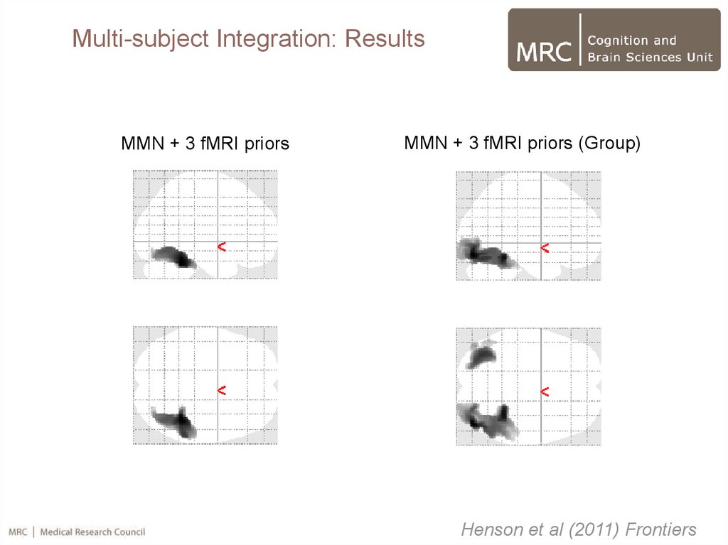
78.
Multi-subject Integration: ResultsMMN + 3 fMRI priors
MMN + 3 fMRI priors (Group)
Henson et al (2011) Frontiers