Assumption of homoscedasticty

1. Assumption of Homoscedasticity

SW388R7
Data Analysis &
Computers II
Assumption of Homoscedasticity
Slide 1
Homoscedasticity
(also referred to as homogeneity of variance)
(also referred to as uniformity of variance)
Transformations
Assumption of normality script
Practice problems

2. Assumption of Homoscedasticity

SW388R7
Data Analysis &
Computers II
Assumption of Homoscedasticity
Slide 2
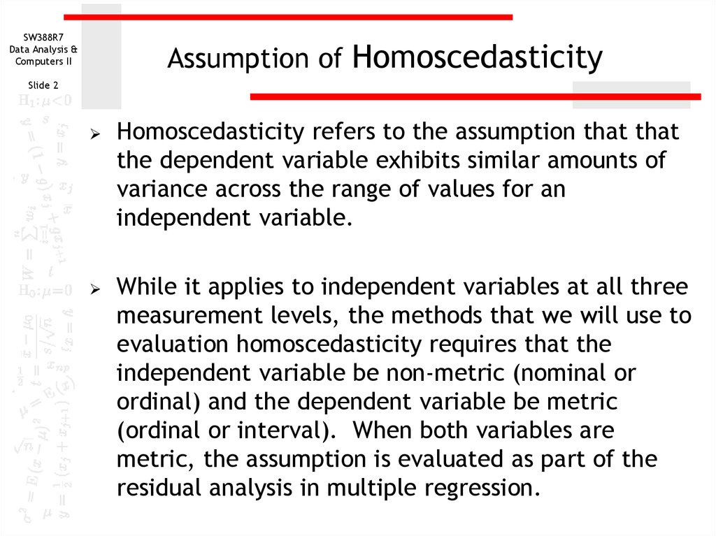
Homoscedasticity refers to the assumption that that
the dependent variable exhibits similar amounts of
variance across the range of values for an
independent variable.
While it applies to independent variables at all three
measurement levels, the methods that we will use to
evaluation homoscedasticity requires that the
independent variable be non-metric (nominal or
ordinal) and the dependent variable be metric
(ordinal or interval). When both variables are
metric, the assumption is evaluated as part of the
residual analysis in multiple regression.

3. Evaluating homoscedasticity

SW388R7
Data Analysis &
Computers II
Evaluating homoscedasticity
Slide 3
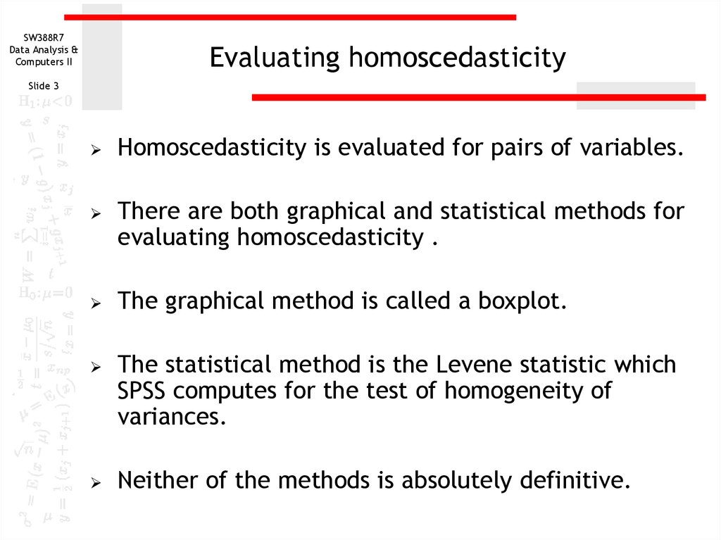
Homoscedasticity is evaluated for pairs of variables.
There are both graphical and statistical methods for
evaluating homoscedasticity .
The graphical method is called a boxplot.
The statistical method is the Levene statistic which
SPSS computes for the test of homogeneity of
variances.
Neither of the methods is absolutely definitive.

4. Transformations

SW388R7
Data Analysis &
Computers II
Transformations
Slide 4
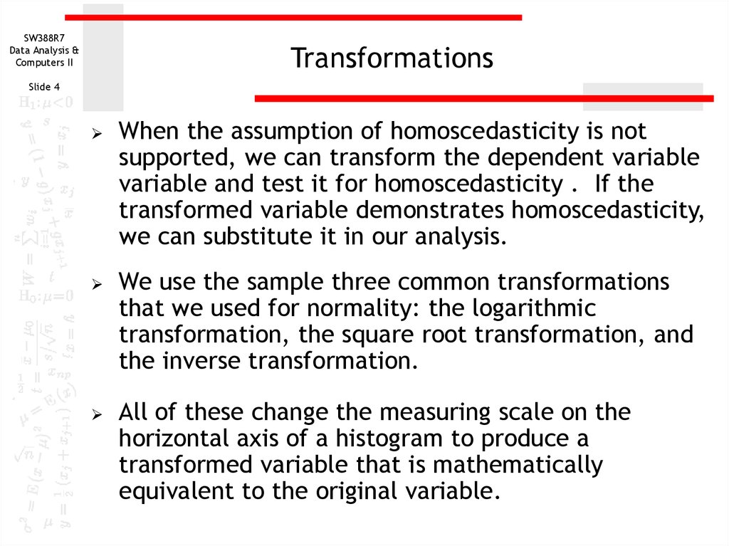
When the assumption of homoscedasticity is not
supported, we can transform the dependent variable
variable and test it for homoscedasticity . If the
transformed variable demonstrates homoscedasticity,
we can substitute it in our analysis.
We use the sample three common transformations
that we used for normality: the logarithmic
transformation, the square root transformation, and
the inverse transformation.
All of these change the measuring scale on the
horizontal axis of a histogram to produce a
transformed variable that is mathematically
equivalent to the original variable.

5. When transformations do not work

SW388R7
Data Analysis &
Computers II
When transformations do not work
Slide 5
When none of the transformations results in
homoscedasticity for the variables in the
relationship, including that variable in the analysis
will reduce our effectiveness at identifying statistical
relationships, i.e. we lose power.

6. Problem 1

SW388R7
Data Analysis &
Computers II
Problem 1
Slide 6
In the dataset GSS2000.sav, is the following
statement true, false, or an incorrect application of
a statistic? Use 0.01 as the level of significance.
Based on a diagnostic hypothesis test for
homogeneity of variance, the variance in "highest
academic degree" is homogeneous for the categories
of "marital status.“
1.
2.
3.
4.
True
True with caution
False
Incorrect application of a statistic

7. Request a boxplot

SW388R7
Data Analysis &
Computers II
Request a boxplot
Slide 7
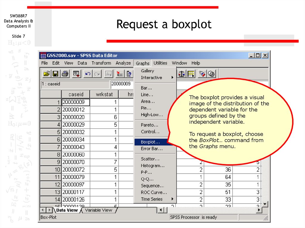
The boxplot provides a visual
image of the distribution of the
dependent variable for the
groups defined by the
independent variable.
To request a boxplot, choose
the BoxPlot… command from
the Graphs menu.

8. Specify the type of boxplot

SW388R7
Data Analysis &
Computers II
Specify the type of boxplot
Slide 8
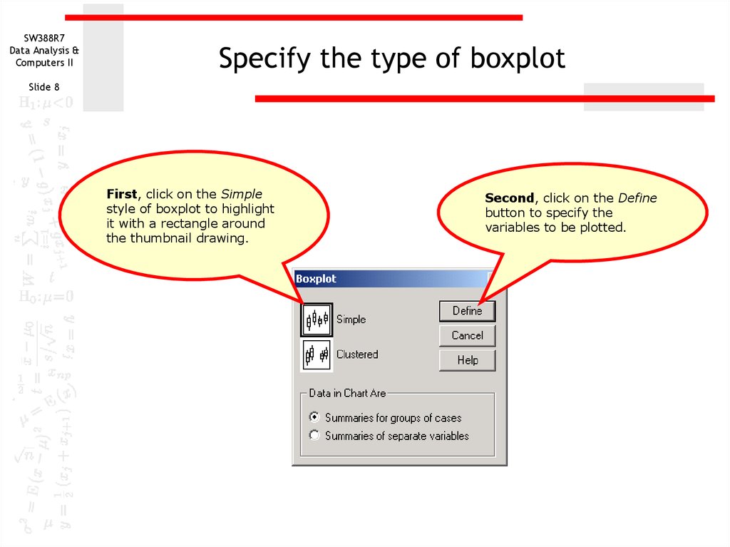
First, click on the Simple
style of boxplot to highlight
it with a rectangle around
the thumbnail drawing.
Second, click on the Define
button to specify the
variables to be plotted.

9. Specify the dependent variable

SW388R7
Data Analysis &
Computers II
Specify the dependent variable
Slide 9
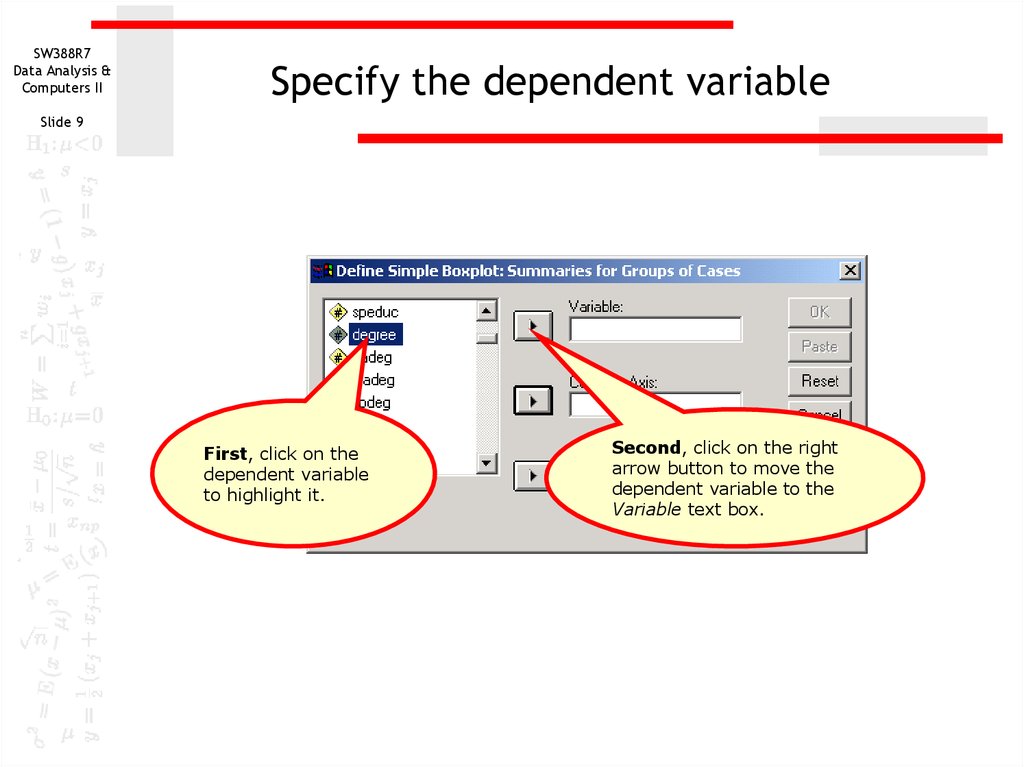
First, click on the
dependent variable
to highlight it.
Second, click on the right
arrow button to move the
dependent variable to the
Variable text box.

10. Specify the independent variable

SW388R7
Data Analysis &
Computers II
Specify the independent variable
Slide 10
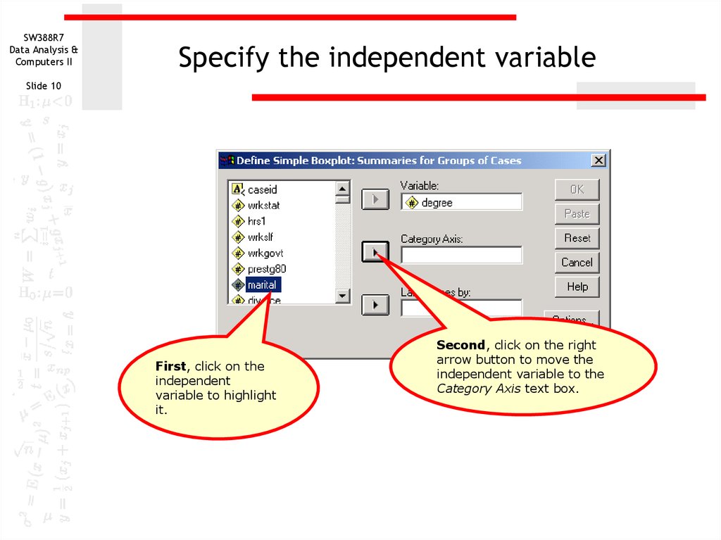
First, click on the
independent
variable to highlight
it.
Second, click on the right
arrow button to move the
independent variable to the
Category Axis text box.

11. Complete the request for the boxplot

SW388R7
Data Analysis &
Computers II
Complete the request for the boxplot
Slide 11
To complete the
request for the
boxplot, click on
the OK button.

12. The boxplot

SW388R7
Data Analysis &
Computers II
The boxplot
Slide 12
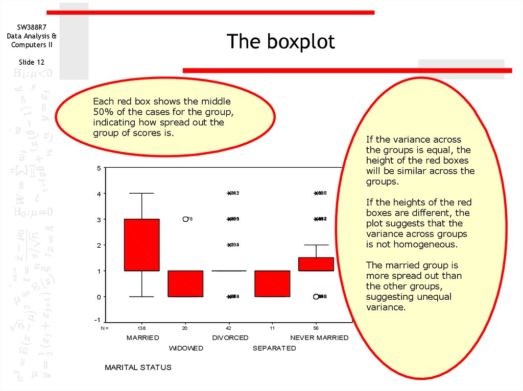
Each red box shows the middle
50% of the cases for the group,
indicating how spread out the
group of scores is.
If the variance across
the groups is equal, the
height of the red boxes
will be similar across the
groups.
5
141
262
4
78
3
2
63
68
197
236
90
100
163
171
181
40
66
69
81
112
217
234
134
203
1
0
243
214
89
87
58
18
9
256
142
132
105
29
-1
N=
138
20
MARRIED
42
DIVORCED
WIDOWED
MARITAL STATUS
11
56
NEVER MARRIED
SEPARAT ED
If the heights of the red
boxes are different, the
plot suggests that the
variance across groups
is not homogeneous.
The married group is
more spread out than
the other groups,
suggesting unequal
variance.

13. Request the test for homogeneity of variance

SW388R7
Data Analysis &
Computers II
Request the test for homogeneity of variance
Slide 13
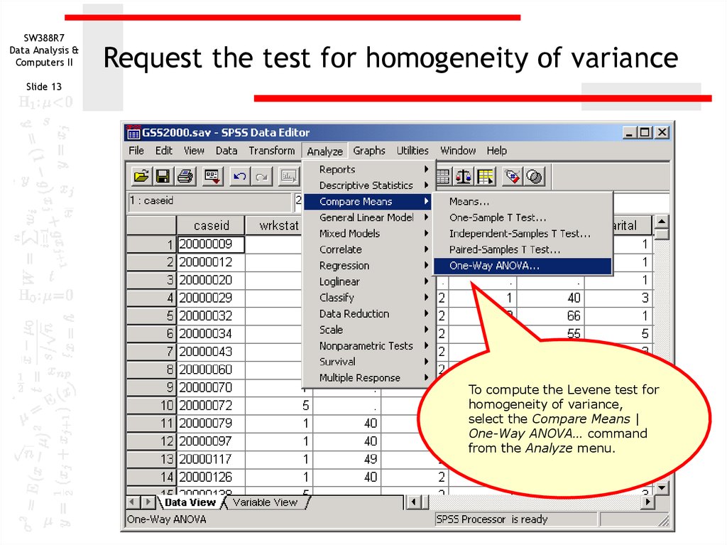
To compute the Levene test for
homogeneity of variance,
select the Compare Means |
One-Way ANOVA… command
from the Analyze menu.

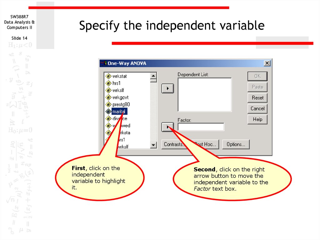
14. Specify the independent variable

SW388R7
Data Analysis &
Computers II
Specify the independent variable
Slide 14
First, click on the
independent
variable to highlight
it.
Second, click on the right
arrow button to move the
independent variable to the
Factor text box.

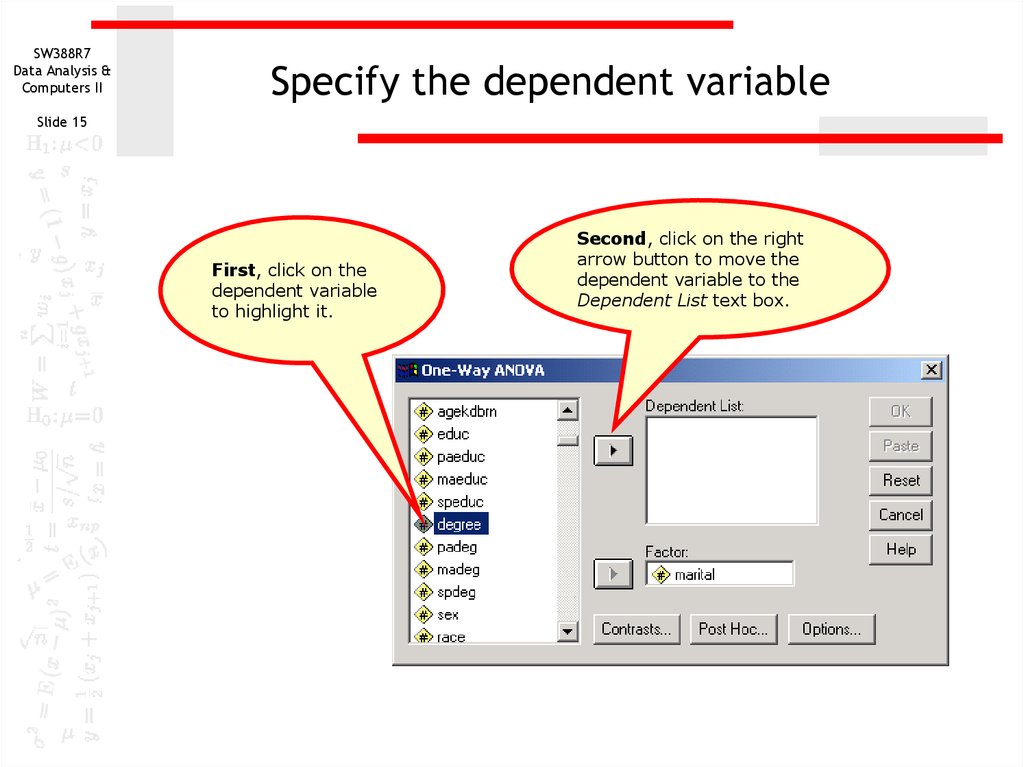
15. Specify the dependent variable

SW388R7
Data Analysis &
Computers II
Specify the dependent variable
Slide 15
First, click on the
dependent variable
to highlight it.
Second, click on the right
arrow button to move the
dependent variable to the
Dependent List text box.

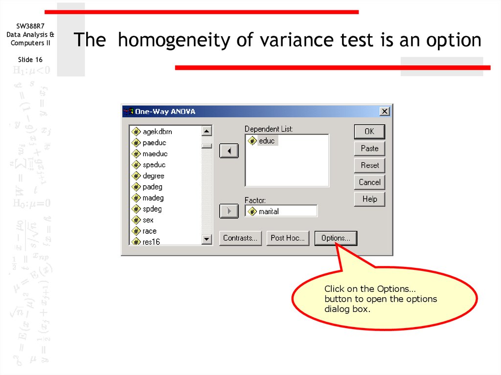
16. The homogeneity of variance test is an option

SW388R7
Data Analysis &
Computers II
The homogeneity of variance test is an option
Slide 16
Click on the Options…
button to open the options
dialog box.

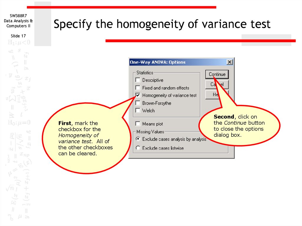
17. Specify the homogeneity of variance test

SW388R7
Data Analysis &
Computers II
Specify the homogeneity of variance test
Slide 17
First, mark the
checkbox for the
Homogeneity of
variance test. All of
the other checkboxes
can be cleared.
Second, click on
the Continue button
to close the options
dialog box.

18. Complete the request for output

SW388R7
Data Analysis &
Computers II
Complete the request for output
Slide 18
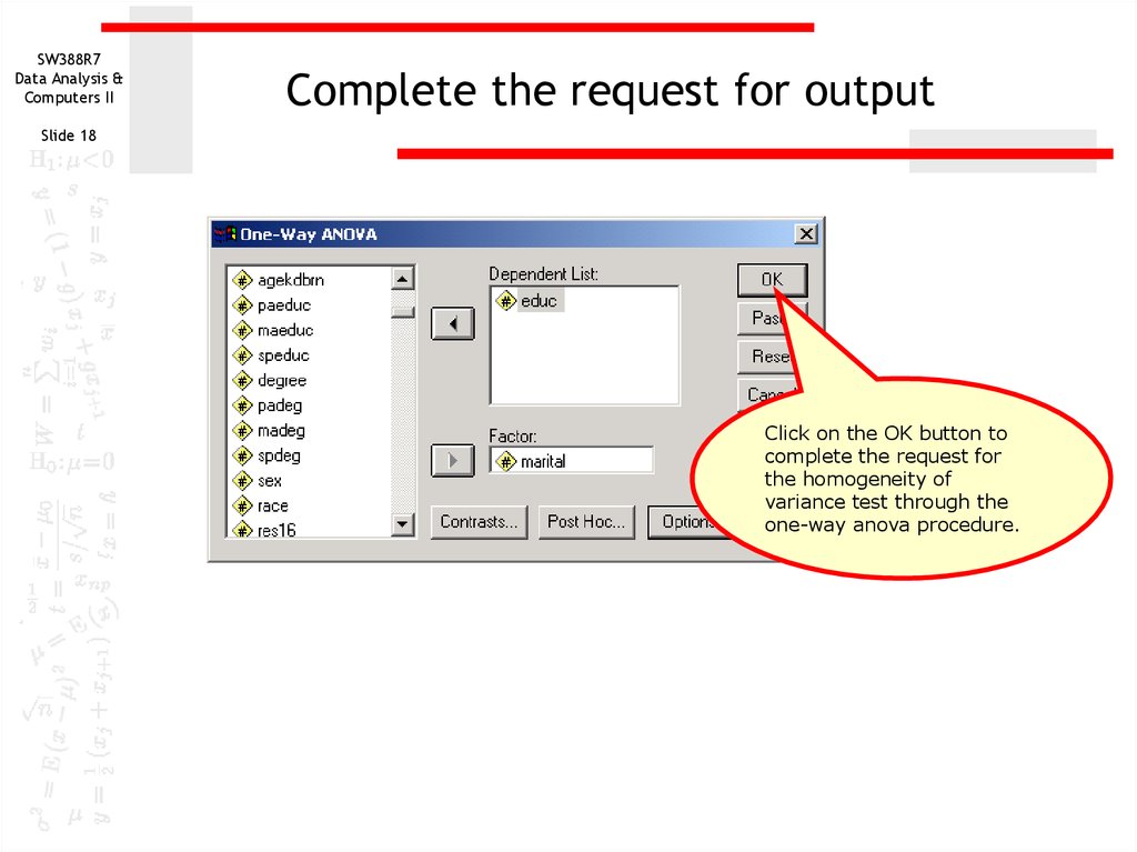
Click on the OK button to
complete the request for
the homogeneity of
variance test through the
one-way anova procedure.

19. Interpreting the homogeneity of variance test

SW388R7
Data Analysis &
Computers II
Interpreting the homogeneity of variance test
Slide 19
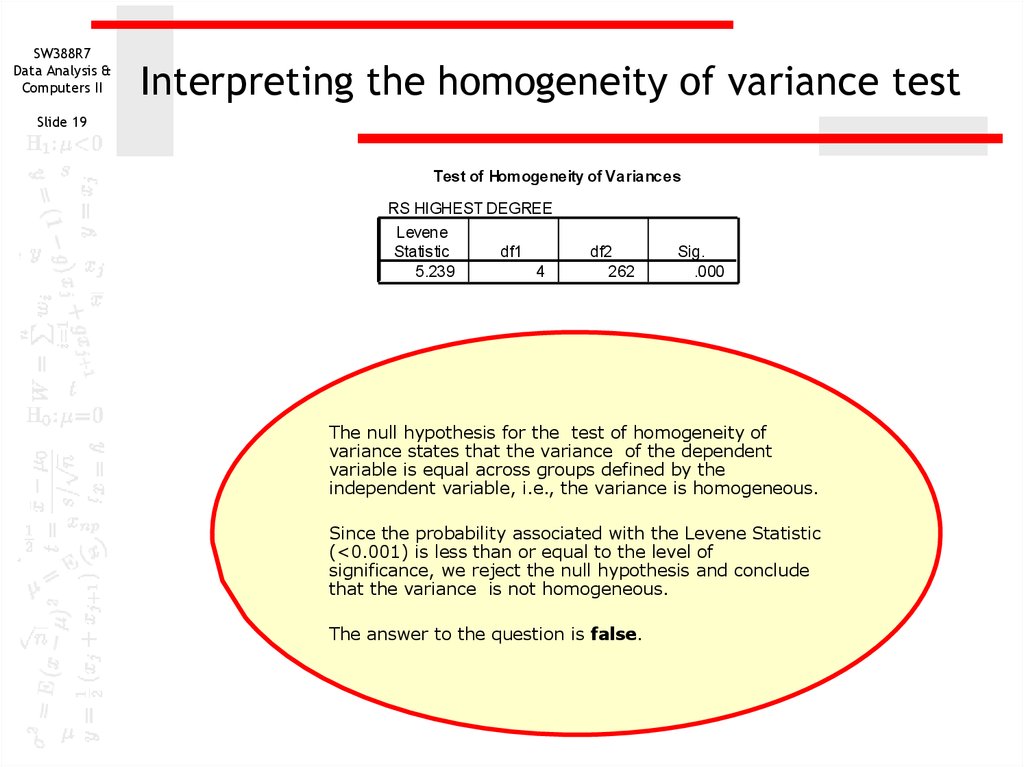
Test of Homogeneity of Variances
RS HIGHEST DEGREE
Levene
Statis tic
5.239
df1
4
df2
262
Sig.
.000
The null hypothesis for the test of homogeneity of
variance states that the variance of the dependent
variable is equal across groups defined by the
independent variable, i.e., the variance is homogeneous.
Since the probability associated with the Levene Statistic
(<0.001) is less than or equal to the level of
significance, we reject the null hypothesis and conclude
that the variance is not homogeneous.
The answer to the question is false.

20. The assumption of homoscedasticity script

SW388R7
Data Analysis &
Computers II
The assumption of homoscedasticity script
Slide 20
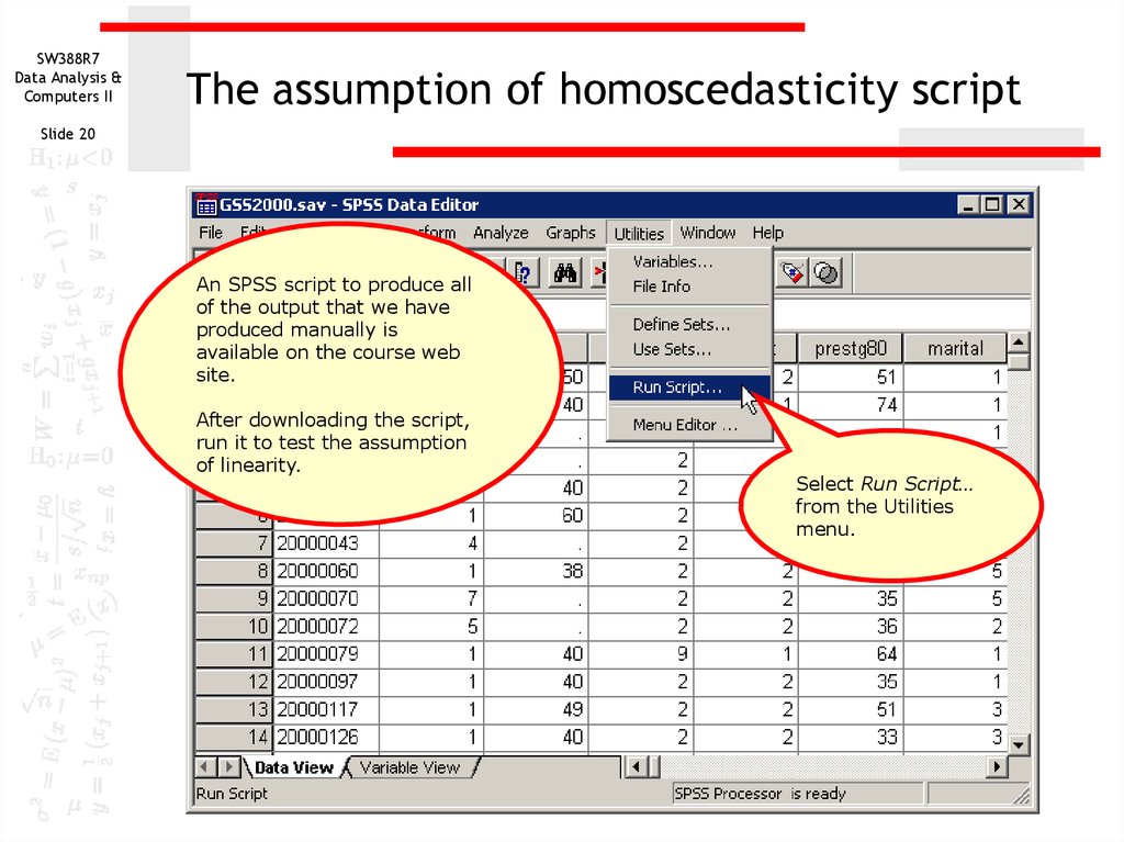
An SPSS script to produce all
of the output that we have
produced manually is
available on the course web
site.
After downloading the script,
run it to test the assumption
of linearity.
Select Run Script…
from the Utilities
menu.

21. Selecting the assumption of homoscedasticity script

SW388R7
Data Analysis &
Computers II
Slide 21
Selecting the assumption of homoscedasticity
script
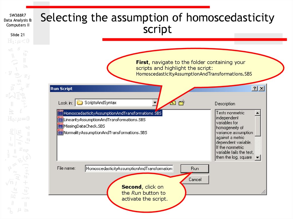
First, navigate to the folder containing your
scripts and highlight the script:
HomoscedasticityAssumptionAndTransformations.SBS
Second, click on
the Run button to
activate the script.

22. Specifications for homoscedasticity script

SW388R7
Data Analysis &
Computers II
Specifications for homoscedasticity script
Slide 22
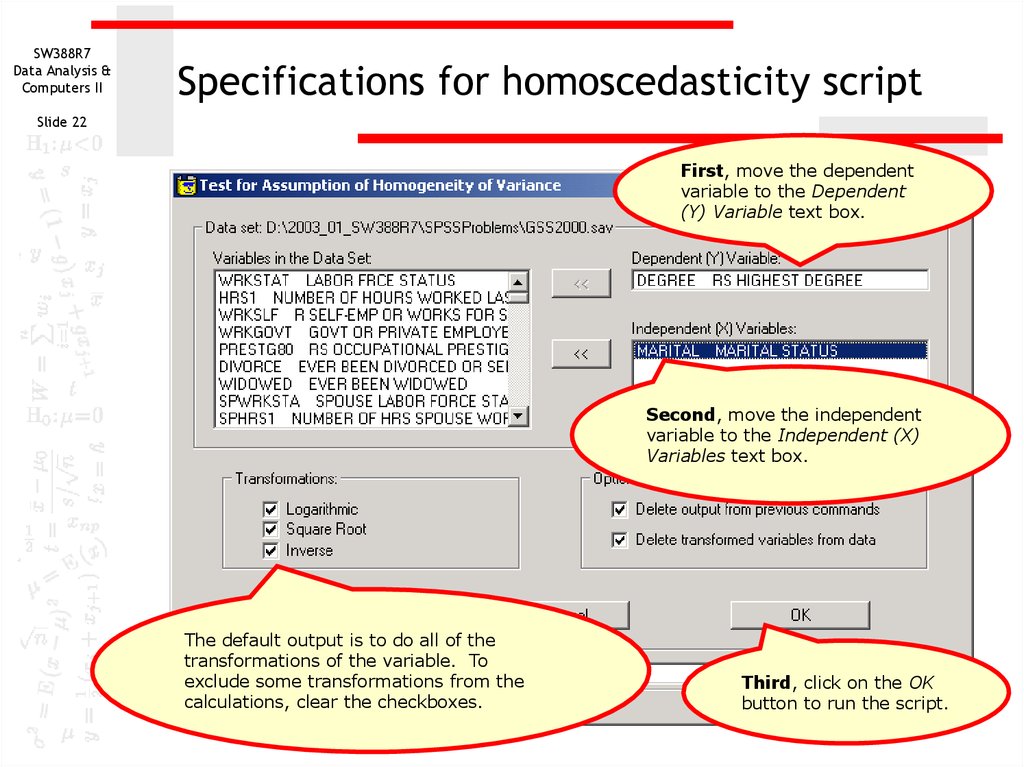
First, move the dependent
variable to the Dependent
(Y) Variable text box.
Second, move the independent
variable to the Independent (X)
Variables text box.
The default output is to do all of the
transformations of the variable. To
exclude some transformations from the
calculations, clear the checkboxes.
Third, click on the OK
button to run the script.

23. The test of homogeneity of variance

SW388R7
Data Analysis &
Computers II
The test of homogeneity of variance
Slide 23
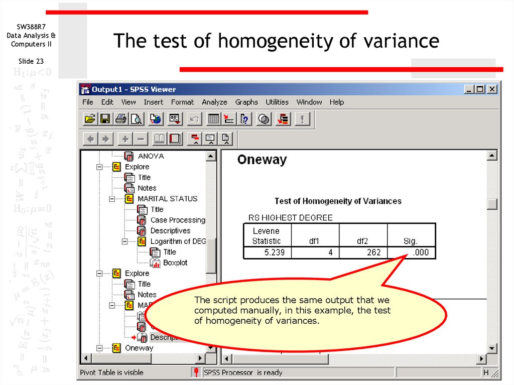
The script produces the same output that we
computed manually, in this example, the test
of homogeneity of variances.

24. Problem 2

SW388R7
Data Analysis &
Computers II
Problem 2
Slide 24
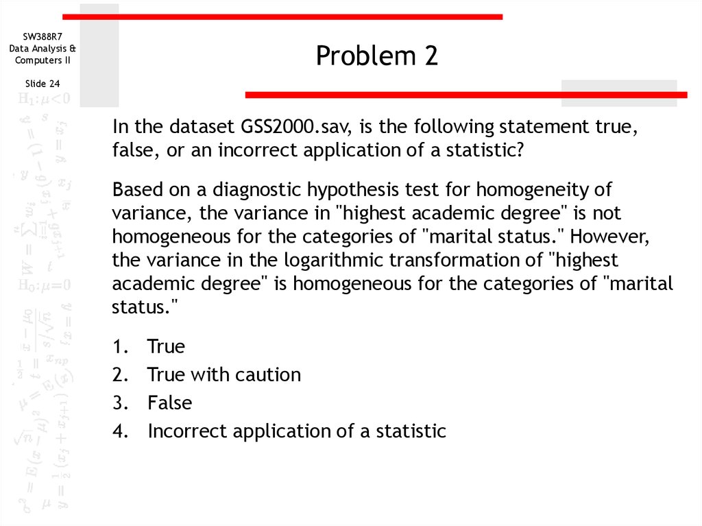
In the dataset GSS2000.sav, is the following statement true,
false, or an incorrect application of a statistic?
Based on a diagnostic hypothesis test for homogeneity of
variance, the variance in "highest academic degree" is not
homogeneous for the categories of "marital status." However,
the variance in the logarithmic transformation of "highest
academic degree" is homogeneous for the categories of "marital
status."
1.
2.
3.
4.
True
True with caution
False
Incorrect application of a statistic

25. Computing the logarithmic transformation

SW388R7
Data Analysis &
Computers II
Computing the logarithmic transformation
Slide 25
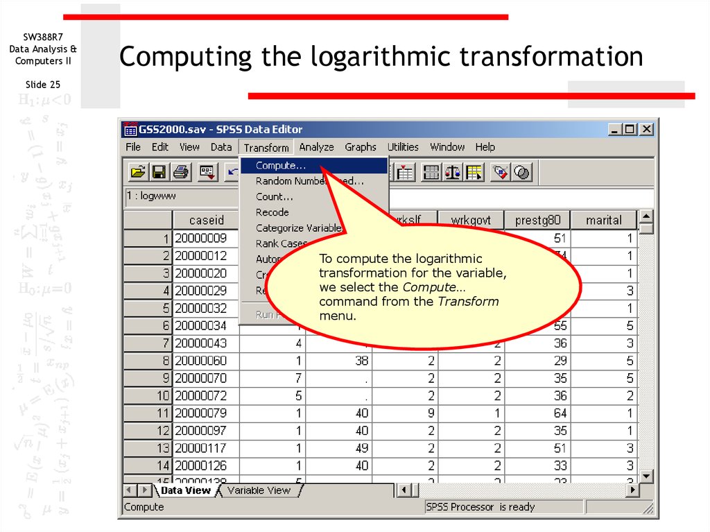
To compute the logarithmic
transformation for the variable,
we select the Compute…
command from the Transform
menu.

26. Specifying the variable name and function

SW388R7
Data Analysis &
Computers II
Specifying the variable name and function
Slide 26
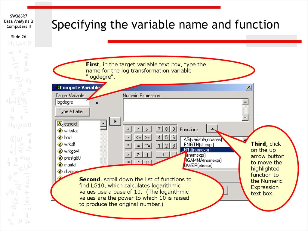
First, in the target variable text box, type the
name for the log transformation variable
“logdegre“.
Second, scroll down the list of functions to
find LG10, which calculates logarithmic
values use a base of 10. (The logarithmic
values are the power to which 10 is raised
to produce the original number.)
Third, click
on the up
arrow button
to move the
highlighted
function to
the Numeric
Expression
text box.

27. Adding the variable name to the function

SW388R7
Data Analysis &
Computers II
Adding the variable name to the function
Slide 27
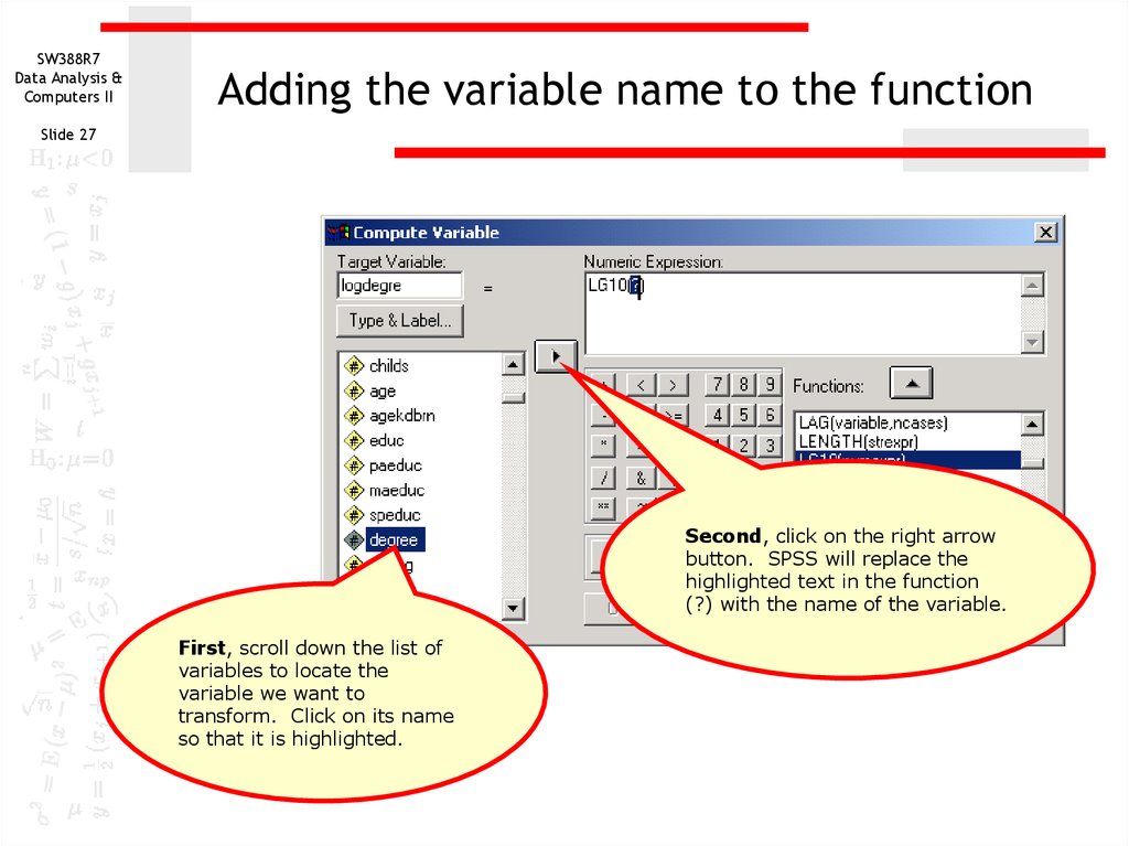
Second, click on the right arrow
button. SPSS will replace the
highlighted text in the function
(?) with the name of the variable.
First, scroll down the list of
variables to locate the
variable we want to
transform. Click on its name
so that it is highlighted.

28. Preventing illegal logarithmic values

SW388R7
Data Analysis &
Computers II
Preventing illegal logarithmic values
Slide 28
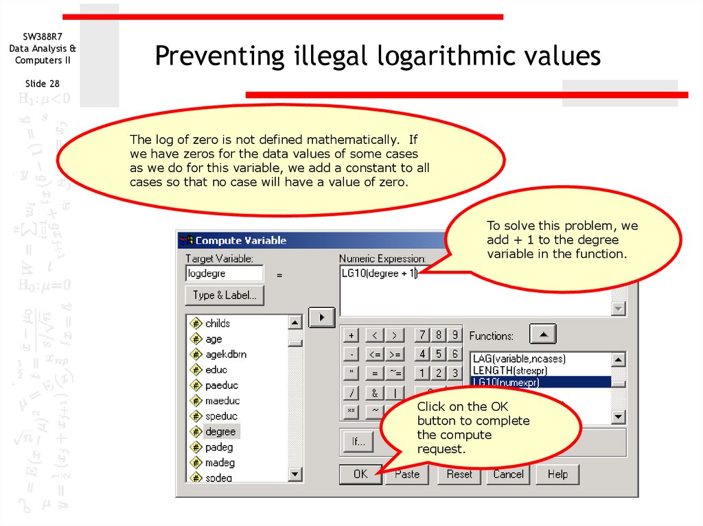
The log of zero is not defined mathematically. If
we have zeros for the data values of some cases
as we do for this variable, we add a constant to all
cases so that no case will have a value of zero.
To solve this problem, we
add + 1 to the degree
variable in the function.
Click on the OK
button to complete
the compute
request.

29. The transformed variable

SW388R7
Data Analysis &
Computers II
The transformed variable
Slide 29
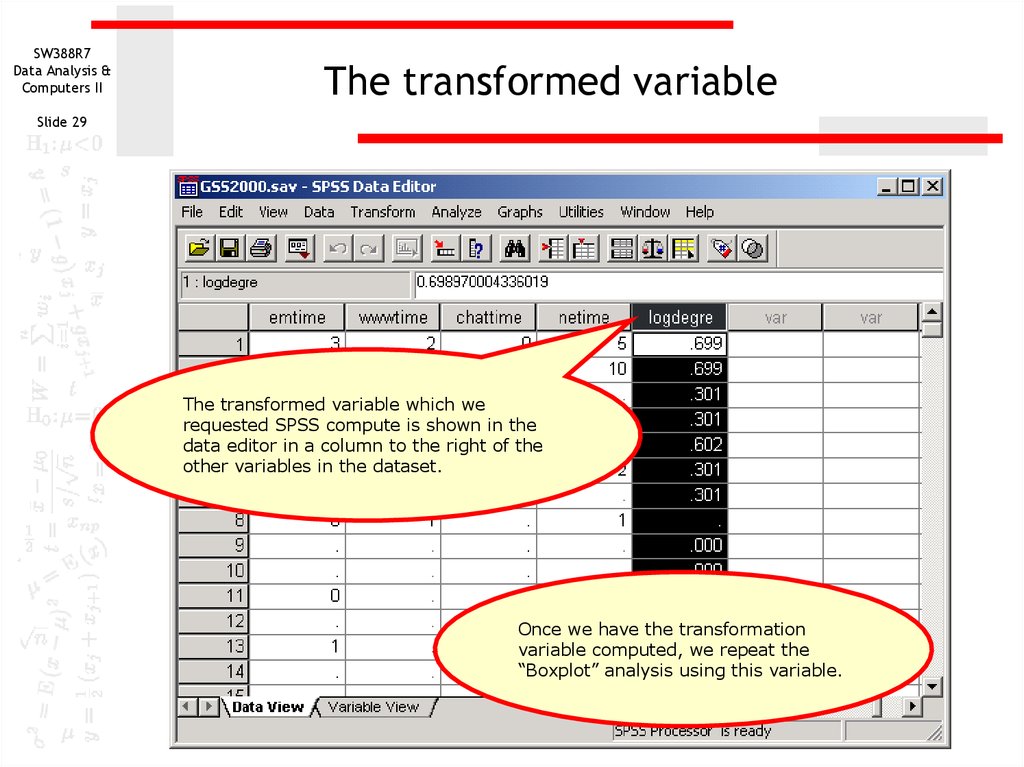
The transformed variable which we
requested SPSS compute is shown in the
data editor in a column to the right of the
other variables in the dataset.
Once we have the transformation
variable computed, we repeat the
“Boxplot” analysis using this variable.

30. The boxplot

SW388R7
Data Analysis &
Computers II
The boxplot
Slide 30
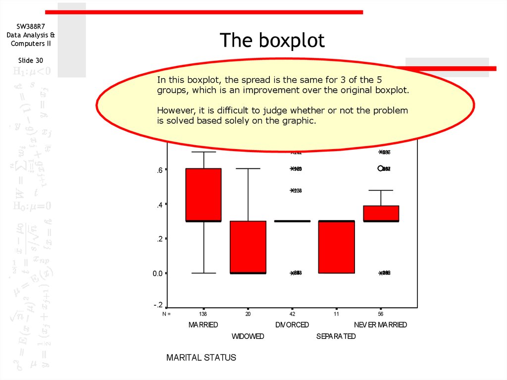
In this boxplot, the spread is the same for 3 of the 5
groups, which is an improvement over the original boxplot.
However, it is difficult to judge whether or not the problem
is solved based solely on the graphic.
.8
.6
141
262
63
68
197
236
90
100
163
171
181
40
66
69
81
112
217
234
134
203
.4
LOGDEGRE
.2
0.0
243
214
89
87
58
18
9
256
142
132
105
29
-.2
N=
138
20
MARRIED
42
DIVORCED
WIDOWED
MARITAL STATUS
11
56
NEVER MARRIED
SEPARATED

31. The homogeneity of variance test

SW388R7
Data Analysis &
Computers II
The homogeneity of variance test
Slide 31
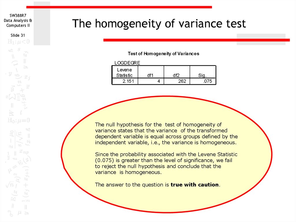
Test of Homogeneity of Variances
LOGDEGRE
Levene
Statis tic
2.151
df1
4
df2
262
Sig.
.075
The null hypothesis for the test of homogeneity of
variance states that the variance of the transformed
dependent variable is equal across groups defined by the
independent variable, i.e., the variance is homogeneous.
Since the probability associated with the Levene Statistic
(0.075) is greater than the level of significance, we fail
to reject the null hypothesis and conclude that the
variance is homogeneous.
The answer to the question is true with caution.

32. Homogeneity of variance test from the script

SW388R7
Data Analysis &
Computers II
Homogeneity of variance test from the script
Slide 32
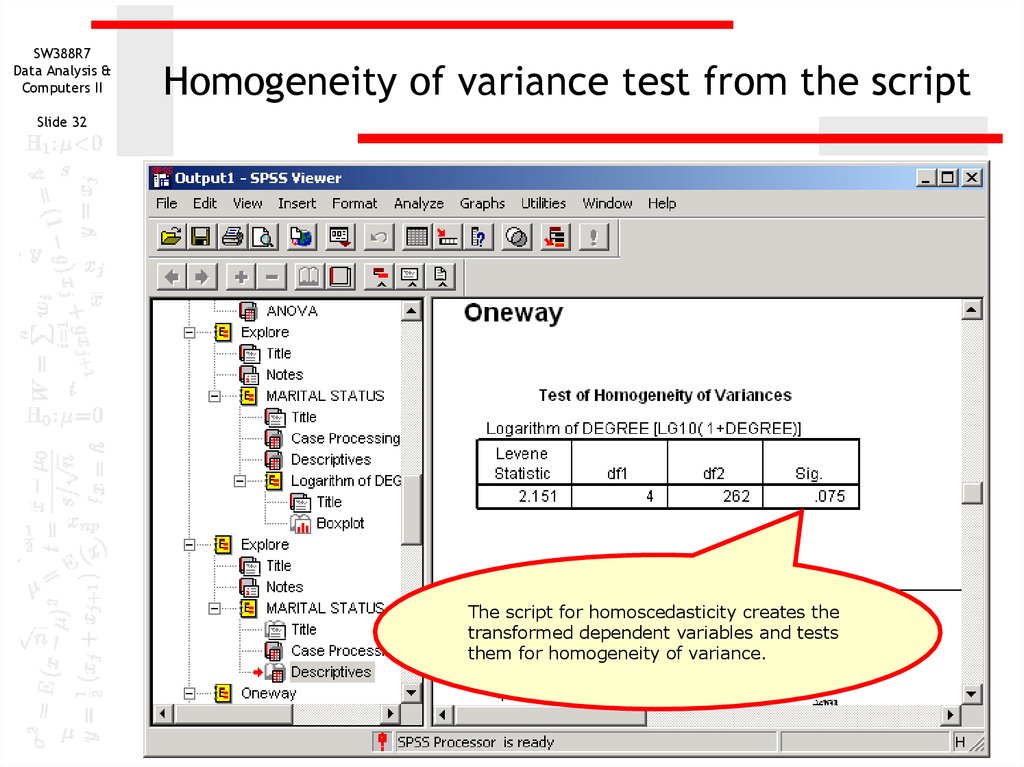
The script for homoscedasticity creates the
transformed dependent variables and tests
them for homogeneity of variance.

33. Other problems on homoscedasticity assumption

SW388R7
Data Analysis &
Computers II
Other problems on homoscedasticity assumption
Slide 33
A problem may ask about the assumption of
homoscedasticity for a nominal level dependent
variable. The answer will be “An inappropriate
application of a statistic” since variance is not
computed for a nominal variable. Similarly, an ANOVA
cannot be calculated if the independent variable is
interval level and the answer will be “An inappropriate
application of a statistic.”
A problem may ask about the assumption of
homoscedasticity for an ordinal level dependent
variable. If the variable or transformed variable
satisfies the assumption of homogeneity of variance,
the correct answer to the question is “True with
caution” since we may be required to defend treating
ordinal variables as metric.

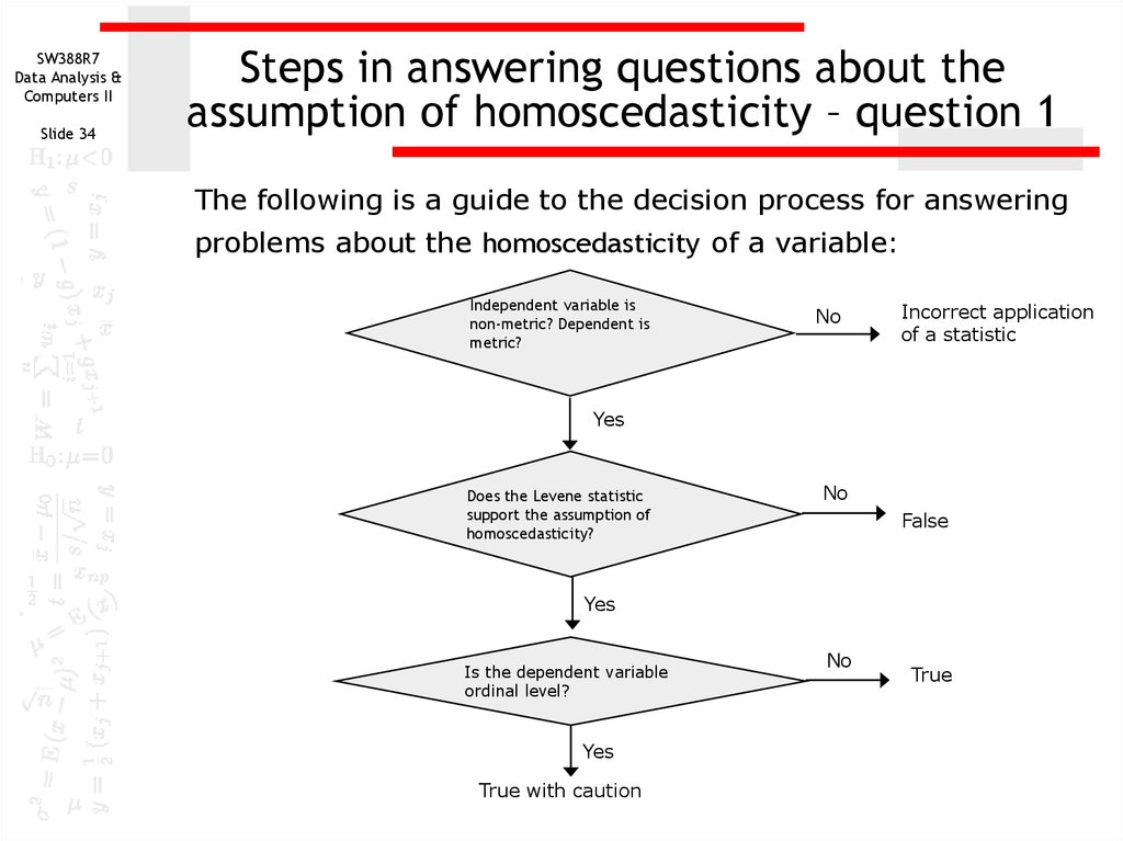
34. Steps in answering questions about the assumption of homoscedasticity – question 1

SW388R7
Data Analysis &
Computers II
Slide 34
Steps in answering questions about the
assumption of homoscedasticity – question 1
The following is a guide to the decision process for answering
problems about the homoscedasticity of a variable:
Independent variable is
non-metric? Dependent is
metric?
No
Incorrect application
of a statistic
Yes
Does the Levene statistic
support the assumption of
homoscedasticity?
No
False
Yes
Is the dependent variable
ordinal level?
Yes
True with caution
No
True

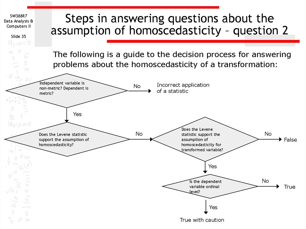
35. Steps in answering questions about the assumption of homoscedasticity – question 2

SW388R7
Data Analysis &
Computers II
Slide 35
Steps in answering questions about the
assumption of homoscedasticity – question 2
The following is a guide to the decision process for answering
problems about the homoscedasticity of a transformation:
Independent variable is
non-metric? Dependent is
metric?
No
Incorrect application
of a statistic
Yes
Does the Levene statistic
support the assumption of
homoscedasticity?
No
Does the Levene
statistic support the
assumption of
homoscedasticity for
transformed variable?
No
False
Yes
Is the dependent
variable ordinal
level?
Yes
True with caution
No
True