Impulse response

1. AUTOMATICS and AUTOMATIC CONTROL

LECTURE 3
dr inż. Adam Kurnicki
Automation and Metrology Department
Room no 210A

2. Slajd 2

Impulse
response
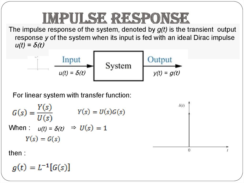
The impulse response of the system, denoted by g(t) is the transient output
response y of the system when its input is fed with an ideal Dirac impulse
u(t) = δ(t)
u(t) = δ(t)
For linear system with transfer function:
When :
then :
u(t) = δ(t)
⇒
y(t) = g(t)

3. Slajd 3

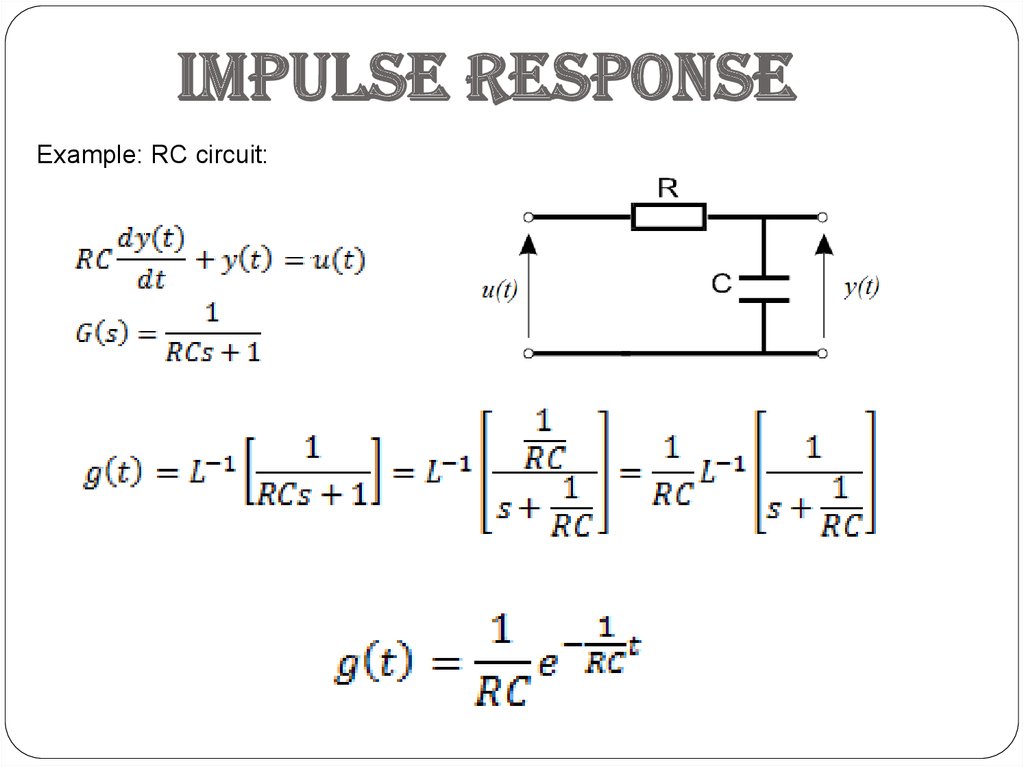
Impulse response
Example: RC circuit:

4. Slajd 4

Step
response
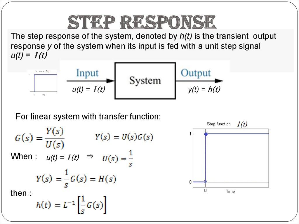
The step response of the system, denoted by h(t) is the transient output
response y of the system when its input is fed with a unit step signal
u(t) = 1(t)
u(t) = 1(t)
For linear system with transfer function:
When :
then :
u(t) = 1(t)
⇒
y(t) = h(t)

5. Slajd 5

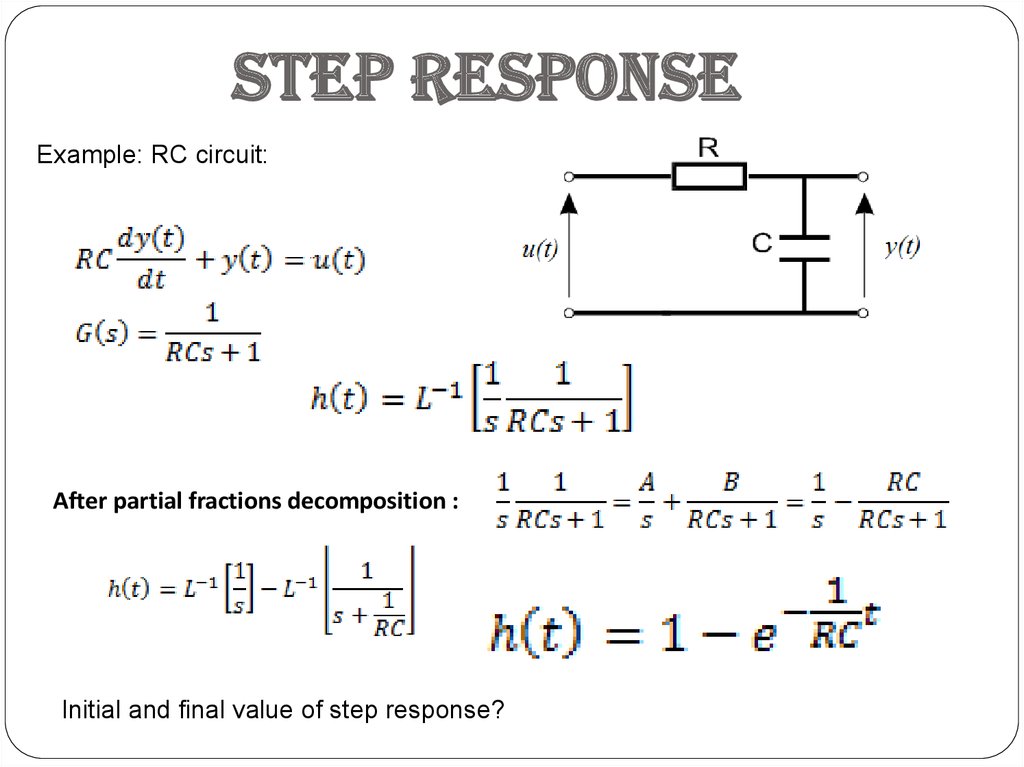
Step response
Example: RC circuit:
After partial fractions decomposition :
Initial and final value of step response?

6. Slajd 6

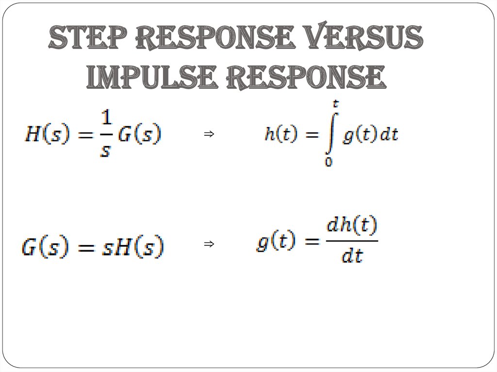
Step response versus
impulse response
⇒
⇒

7. Slajd 7

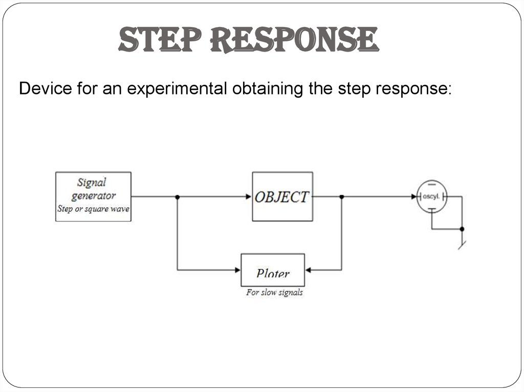
Step response
Device for an experimental obtaining the step response:

8. Slajd 8

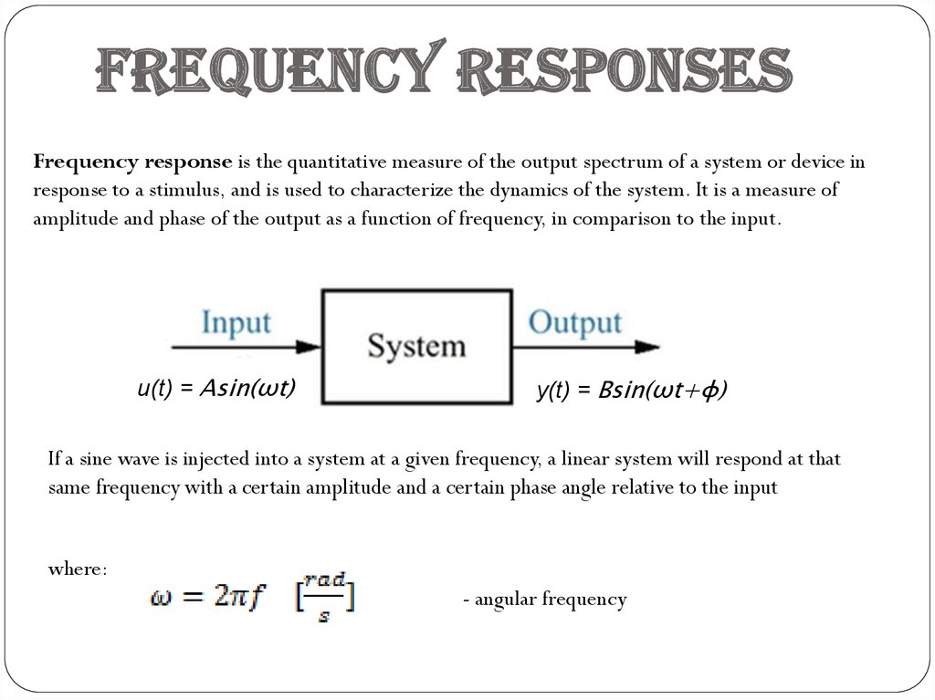
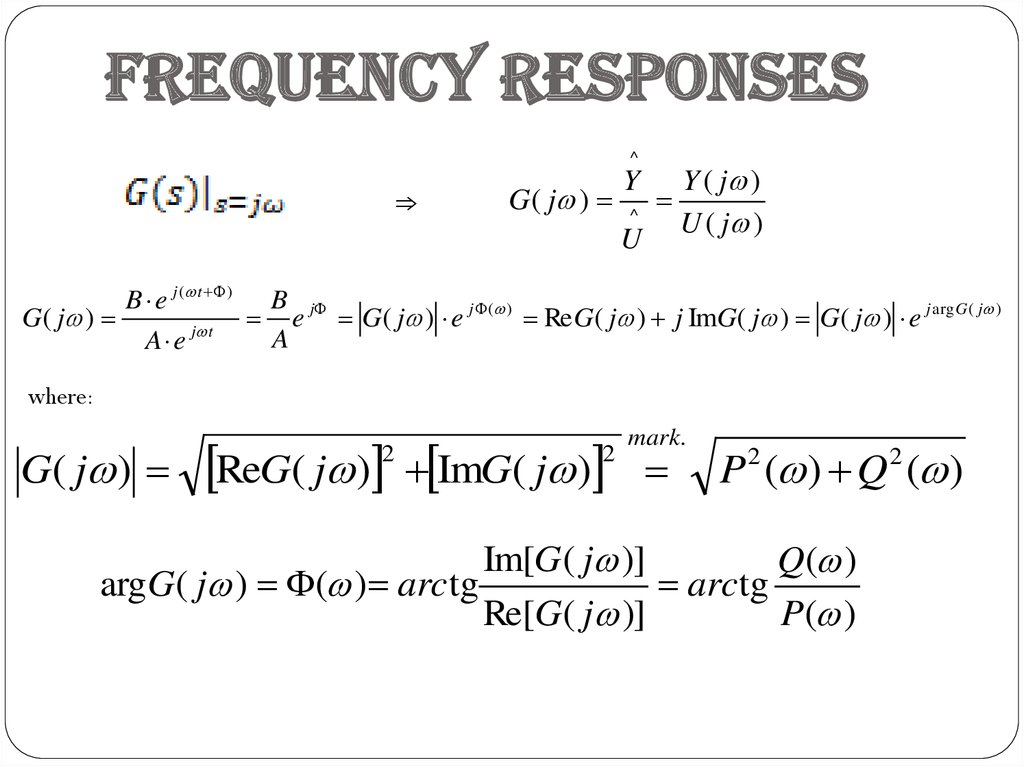
Frequency responses
Frequency response is the quantitative measure of the output spectrum of a system or device in
response to a stimulus, and is used to characterize the dynamics of the system. It is a measure of
amplitude and phase of the output as a function of frequency, in comparison to the input.
u(t) = Asin(ωt)
y(t) = Bsin(ωt+φ)
If a sine wave is injected into a system at a given frequency, a linear system will respond at that
same frequency with a certain amplitude and a certain phase angle relative to the input
where:
- angular frequency

9. Slajd 9

Frequency responses
^
⇒
G ( j )
Y
^
U
Y ( j )
U ( j )
B e j ( t ) B j
j ( )
j arg G ( j )
G( j )
e
G
(
j
)
e
Re
G
(
j
)
j
Im
G
(
j
)
G
(
j
)
e
A
A e j t
where:
G( j )
ReG( j ) ImG( j )
2
2
mark.
P 2 ( ) Q 2 ( )
Im[G( j )]
Q( )
argG( j ) ( ) arc tg
arc tg
Re[G( j )]
P( )

10. Slajd 10

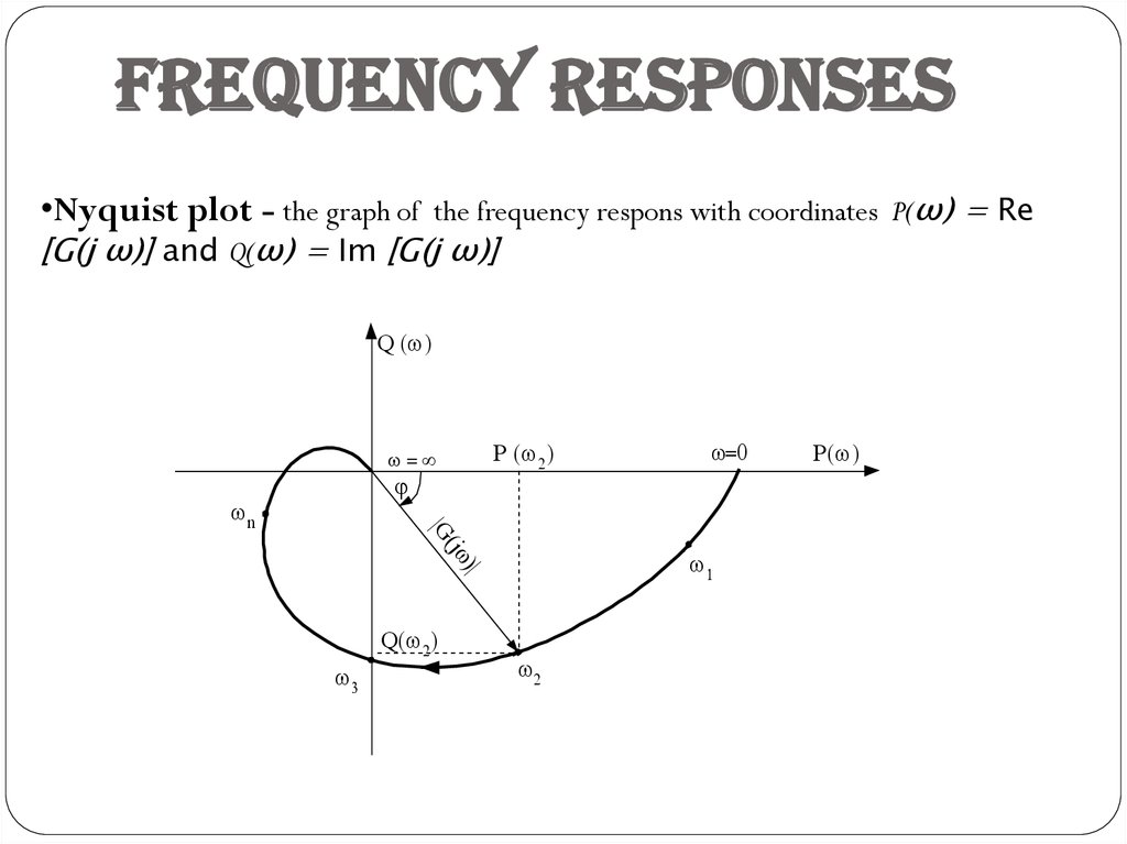
Frequency responses
•Nyquist plot - the graph of the frequency respons with coordinates P(ω) = Re
[G(j ω)] and Q(ω) = Im [G(j ω)]
Q
=
j
G
n
P
Q
P

11. Slajd 11

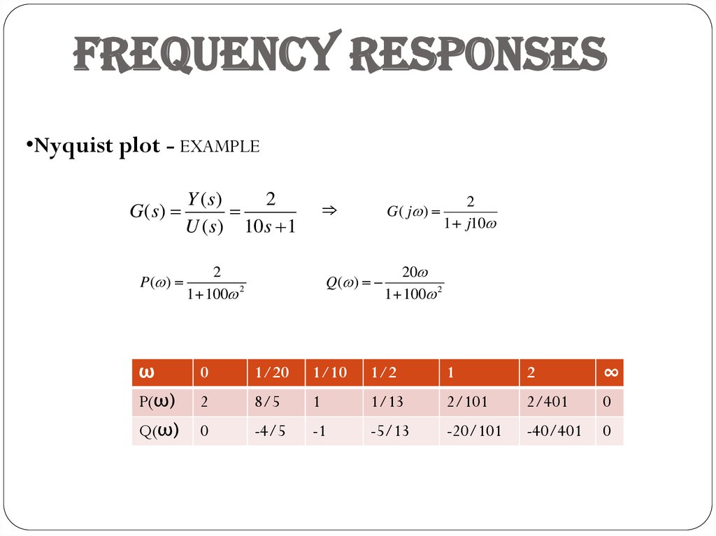
Frequency responses
•Nyquist plot - EXAMPLE
G( s)
P( )
Y ( s)
2
U ( s) 10s 1
⇒
2
1 100 2
G ( j )
Q( )
2
1 j10
20
1 100 2
ω
0
1/20
1/10
1/2
1
2
∞
P(ω)
2
8/5
1
1/13
2/101
2/401
0
Q(ω)
0
-4/5
-1
-5/13
-20/101
-40/401
0

12. Slajd 12

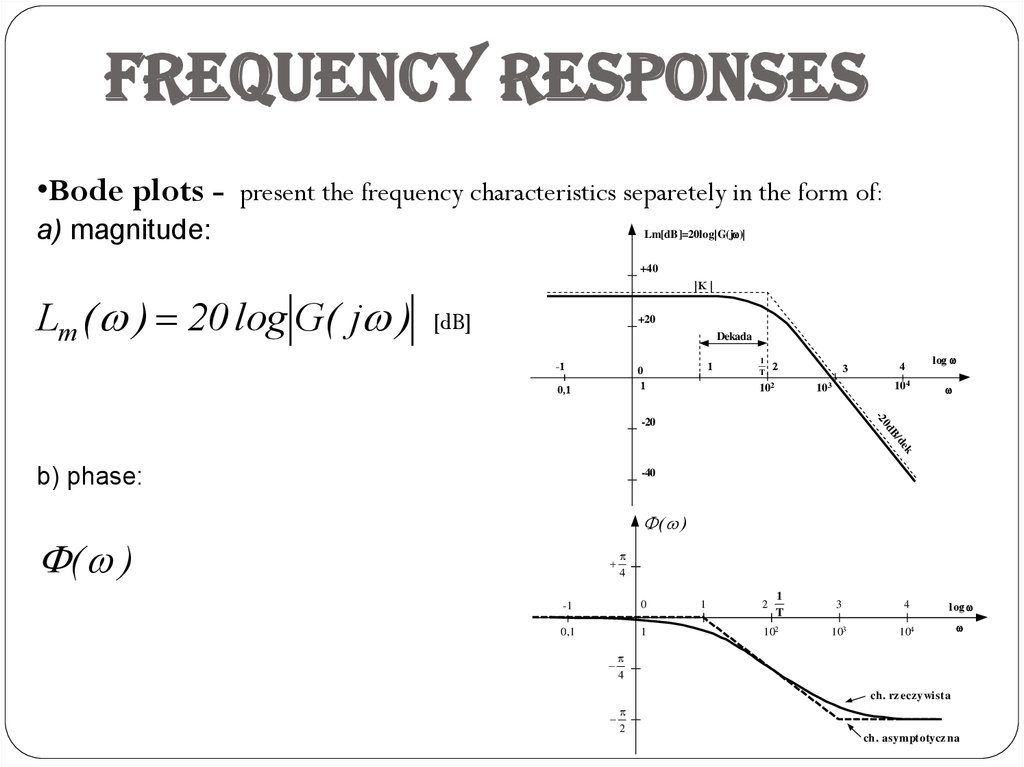
Frequency responses
•Bode plots - present the frequency characteristics separetely in the form of:
a) magnitude:
Lm[dB]=20log G(j )
+40
Lm ( ) 20 log G( j )
K
[dB]
+20
Dekada
-1
1
0
1
0,1
1
T
2
102
4
3
104
103
log
0
-2
dB
-20
/d
ek
b) phase:
-40
( )
( )
4
-1
0
0,1
1
1
2
1
T
102
3
4
log
103
104
4
ch. rz eczywista
2
ch. asym ptotycz na

13. Slajd 13

Frequency responses
•Bode plots - EXAMPLE
G( s)
Y ( s)
k
U ( s) Ts 1
⇒
G( j )
k
1 j T
k
k
k
Lm ( ) 20 log G ( j ) 20 log
20 log
20 log
2
2
1 j T
1 j T
1 T
20 log k 20 log 1 2T 2
0
for T 1
20 log 2T 2 1
- 20log( T) for T 1
- 20log( T) 20 log 20 log T
when :
1/ T
then : - 20log( T) 0
P ( )
k
1 T
( ) arctg
2
2
Q( )
k T
1 2T 2
Q( )
arctg ( T ) arctg ( T )
P( )

14. Slajd 14

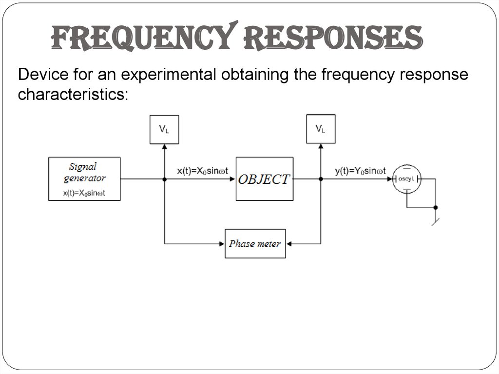
Frequency responses
Device for an experimental obtaining the frequency response
characteristics:

15. Slajd 15

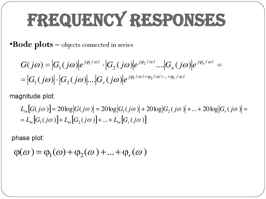
Frequency responses
•Bode plots – objects connected in series
G( j ) G1 ( j ) e j 1 / / G2 ( j ) e j 2 / / .... Gn ( j ) e j n / /
G1 ( j ) G2 ( j ) .... Gr ( j ) e j 1 / / / r / /
magnitude plot:
Lm G( j ) 20 log G( j ) 20 log G1 ( j ) 20 log G2 ( j ) ... 20 log Gr ( j )
Lm G1 ( j ) Lm G2 ( j ) ... Lm Gr ( j )
phase plot:
( ) ( ) ( ) r ( )

16. Slajd 16

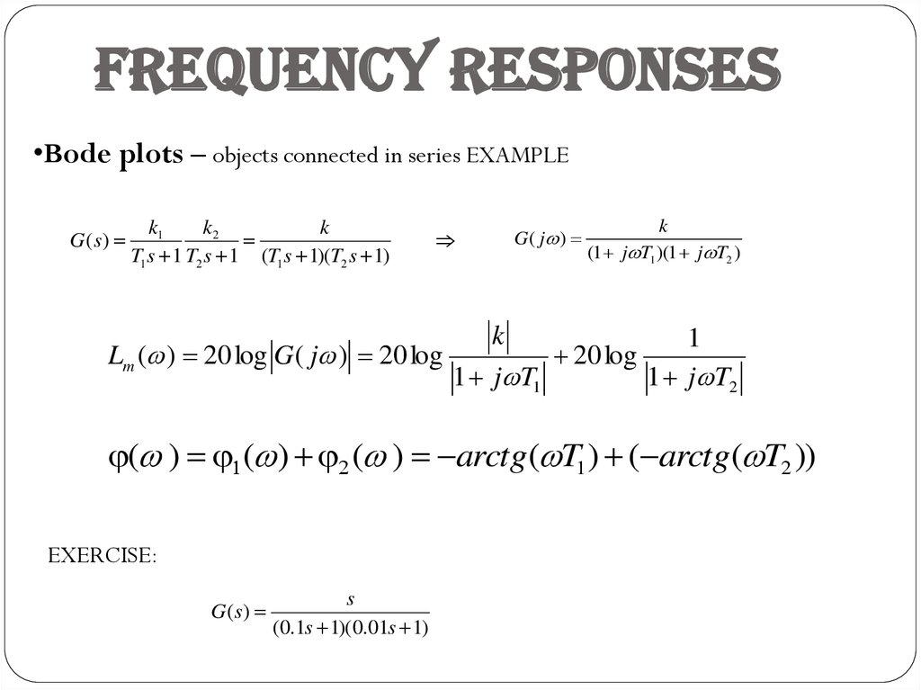
Frequency responses
•Bode plots – objects connected in series EXAMPLE
G(s)
k1
k2
k
T1s 1 T2 s 1 (T1s 1)(T2 s 1)
⇒
G ( j )
k
(1 j T1 )(1 j T2 )
k
1
Lm ( ) 20 log G ( j ) 20 log
20 log
1 j T1
1 j T2
( ) ( ) ( ) arctg( T1 ) ( arctg( T2 ))
EXERCISE:
G( s)
s
(0.1s 1)(0.01s 1)

17. THANK YOU