


 Block Diagram Transformations")


 rise time; (b) overshoot; (c) settling time; (d) composite of all three requirements")


 physics
 electronics
Similar presentations:


")


Control systems
1.
Control SystemsDynamic Response: Dynamic Response
Analysis, Steady State Error
Md Hazrat Ali
Department of Mechanical Engineering,
School of Engineering,
Nazarbayev University
2.
By failing to prepare, you arepreparing to fail.
Benjamin Franklin
3.
Contents-Review of Previous Lectures
-System Response Analysis
4. Review
• Once transfer function is obtained, we can startto analyze the response of the system it
represents .
• A block diagram is a convenient tool to visualize
the systems as a collection of interrelated
subsystems that emphasize the relationships
among the system variables.
• Signal flow graph and Mason’s gain formula are
used to determine the transfer function of the
complex block diagram.
5. Review-Block Diagram
• Three Elementary Block Diagrams– Series connection
– Parallel connection
– Negative Feedback connection
6. Negative feedback :Single-loop gain
The gain of a single-loop negative feedback system isgiven by the forward gain divided by the sum of 1 plus the
loop gain.
Franklin et.al- pp.122
7. Review-Block Diagram
8. Table 2.6 (continued) Block Diagram Transformations
Review-Block DiagramTable 2.6 (continued) Block Diagram Transformations
9. Review-Block Diagram
Practice: Find the transfer function of thefollowing block diagram
Y(s)
2s 4
2
R (s) s 2s 4
10. Review-Block Diagram
Practice:11. Review-Block Diagram
12.
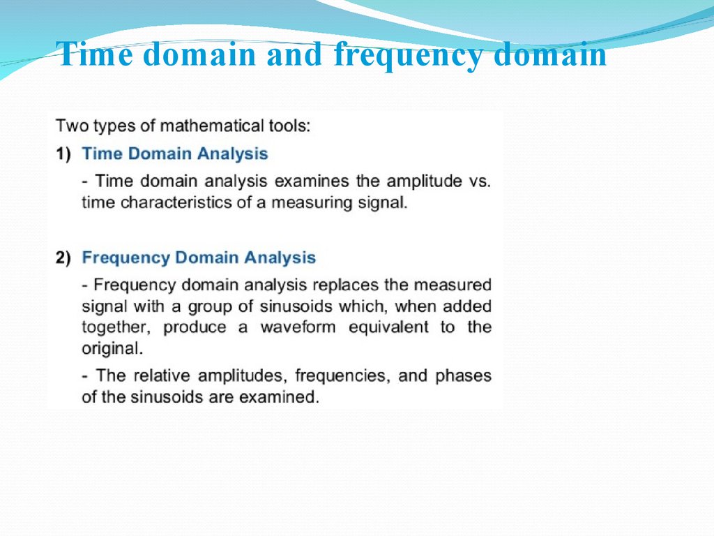
Time domain and frequency domain13.
14.
15.
16.
17. Poles and Zeros
H (s) Km
i 1
n
i 1
( s zi )
( s pi )
K is the transfer gain
The roots of numerator is called zeros of the system. Zeros
correspond to signal transmission-blocking properties.
The roots of denominator are called poles of the system. Poles
determine the stability properties and natural or unforced
behavior of the system.
Poles and zeros can be complex quantities.
zi=pi, cancellation of pole-zero may lead to undesirable system
properties.
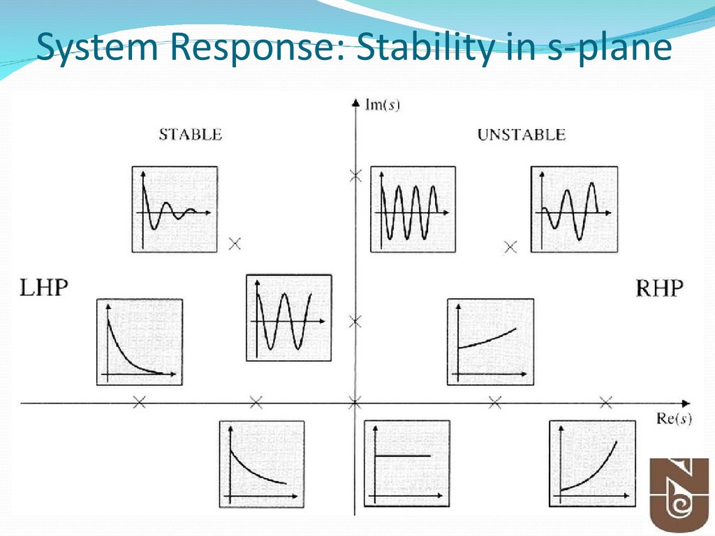
18. System Response: Complex system
19.
20.
Key points: Effect of Poles and Zeros21. System Response
Example:Consider the following transfer function
Y (s)
2s 1
2
R ( s ) s 3s 2
Determine:
• Poles and Zeros?
21
22. System Response: Effect of pole location
23. System Response
Example:Consider the following transfer function
Y ( s)
s 3
2
R ( s ) s 5s 6
Determine:
• Poles and Zeros?
23
24. Time-Domain Specification
Test Input Signals• To measure the performance of a system we use
standard test input signals. This allows us to compare
the performance of our system for different designs.
• The standard test inputs used are the step input, the
ramp input, and the parabolic input.
• A unit impulse function is also useful for test signal
purpose.
25. Time-Domain Specification
Test Input Signalsstep input
ramp input
parabolic input
A, t 0
r (t )
0, t 0
A
R( s)
s
At , t 0
r (t )
0, t 0
A
R( s) 2
s
At 2 , t 0
r (t )
0, t 0
2A
R( s) 3
s
The step input is the easiest to generate and evaluate and is
usually chosen for performance tests.
26. Time-Domain Specification
ExampleThe transfer function:
9
G (s)
s 10
The system response to a unit step input (A=1):
y (t ) 0.9 1 e 10t
y ( ) 0.9
27. System Response
Example 2:Consider the following transfer function
Y ( s)
7s 1/ 2
2
R ( s ) s 5s 6
Determine:
• impulse response
28.
First Order System Response29.
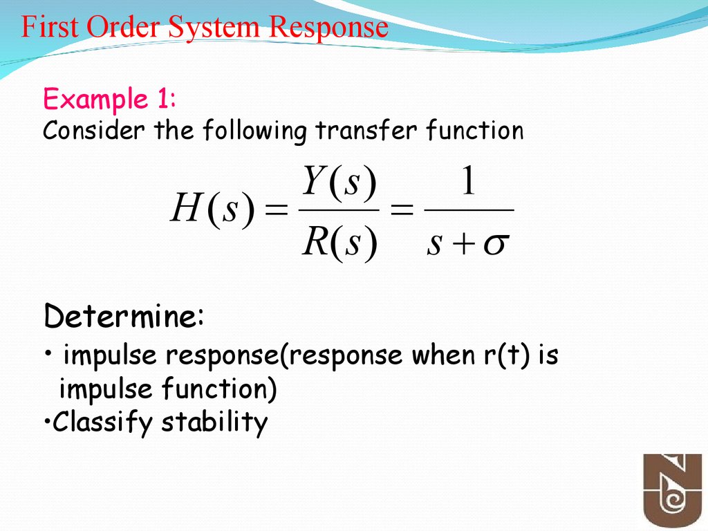
First Order System ResponseExample 1:
Consider the following transfer function
Y (s)
1
H (s)
R(s) s
Determine:
• impulse response(response when r(t) is
impulse function)
•Classify stability
30.
First Order System Response- Impulse response1/
31.
Standard Second Order System• Let us consider the following closed-loop system:
• The TF of the closed-loop system:
G(s)
K
T ( s)
2
1 G ( s ) s ps K
• Utilizing the general notation of 2nd Order System:
T (s) 2
s 2 n s n2
2
n
• Where n is natural frequency and is damping ratio
32.
Standard Second Order Systemd n 1
2
cos 1
0 1
33. Figure 3.24 Graphs of regions in the s-plane delineated by certain transient requirements: (a) rise time; (b) overshoot; (c) settling time; (d) composite of all three requirements
Transformation of the specification to the splaneFigure 3.24 Graphs of regions in the s-plane delineated by certain transient requirements: (a) rise time; (b) overshoot;
(c) settling time; (d) composite of all three requirements
34. Transformation of the specification to the s-plane
Example 3.25Find allowable regions in the s-plane for the poles
transfer function of system if the system response
requirements are tr ≤ 0.6, Mp <= 10% and ts <= 3 sec.
35.
Standard Second Order SystemMp?
36.
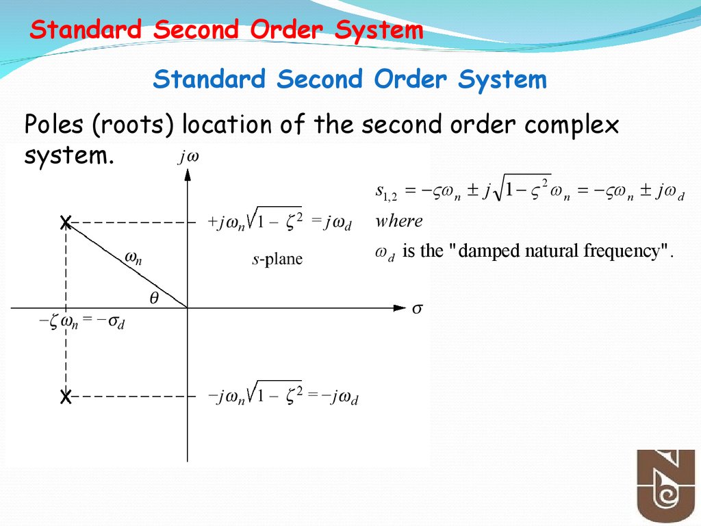
Standard Second Order SystemStandard Second Order System
Poles (roots) location of the second order complex
system.
s1,2 n j 1 2 n n j d
where
d is the "damped natural frequency".
37.
Standard Second Order System• Classification of Type Response of 2nd Order Systems
Undamped: =0
Critical damped: =1
Under-damped: 0< <1
Over-damped: >1
38.
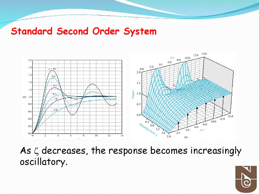
Standard Second Order SystemAs decreases, the response becomes increasingly
oscillatory.
39. Time-Domain Specification
• Standard performance measures are usually defined in termof the step response of a 2nd order systems:
40. Time-Domain Specification
• Standard performance measures are usually definedin term of the step response of a 2nd order systems:
– Rise time, Tr : time needed from 0 to 100% of fv for
underdamped systems and Tr1 from 1090% of fv for
overdamped systems.
– The settling time ts is the time it takes the system transient
to decay.
– The overshoot Mp is the maximum amount of the system
overshoots its final value divided by its final value.
– The peak time tp, is the time it takes the system to reach
the maximum overshoot.
41. Time-Domain Specification
-Rise Time, Tr-A precise analytical relationship between rise time
and damping ratio cannot be found. However, it
can be found using numerically using computer.
A rough estimation of the rise time is as follows
1.8
tr
n
42. Time-Domain Specification
-Maximum Overshoot, MpMaximum overshoot (in percentage) is defined as
Mp
' Peak Value ' ' Final Value '
100%
' Final Value '
M p 100e
1 2
43. Time-Domain Specification
-Peak Time TpTp is found by differentiating y(t) and finding thefirst zero crossing after t=0.
Tp
d n 1 2
44. Time-Domain Specification
-Settling Time Ts-For a second order system, we seek to determine the
time Ts for which the response remains within
certain percentage (1%, 2% ) of the final value.
For 1% settling time
4.6.6
4
Ts
T
s
n n
For 2% settling time
4
Ts
n
45. Time-Domain Specification
Exercise # 1Find Tr, Tp, Mp and Ts for the following transfer
function:
25
T (s) 2
s 30 s 225
45
46. Time-Domain Specification
Exercise # 2Find Tr, Tp, Mp and Ts for the following transfer
function:
19
T (s) 2
s 24 s 19 / 3
46
47. Exercise # 3
If the system response requirements are tr = 0.6, Mp =10% and ts = 3 sec.
Find:
n ,
47
48. Exercise # 4
Problem# If the system response requirements are tr =0.6, Mp = 10% and ts = 3 sec.
Find:
n ,
For 1% settling time
1.8
tr
n
4.6
Ts
n
48
49. Time-Domain Specification
Exercise # 5Find Tr, Tp, Mp and Ts for the following transfer
function:
1
T (s) 2
s 15s 100
50. Time-Domain Specification
Exercise # 6Find Tr, Tp, Mp and Ts for the following transfer
function:
5
T (s) 2
s 30 s 225
50
51. Time-Domain Specification
Exercise # 7Find Tr, Tp, Mp and Ts for the following transfer
function:
3
T (s) 2
s 24 s 9
51
52. Figure - Multiple-loop feedback control system.
Example - Block diagramFind TF from the given block diagram
Figure - Multiple-loop feedback control system.
53. Figure 2.27 Block diagram reduction of the system of Figure 2.26.
Quiz # 4- Answer to Q1Figure 2.27 Block diagram reduction of the system of Figure 2.26.
54. System Response
Find TF from the given block diagramConsider the following transfer function
Y (s)
2s 1
H (s)
2
R ( s ) s 3s 2
Determine:
i) Impulse response graphically
ii) Classify stability
55. Impulse response
Answer56. Midterm Exam
March 4, 2016, Friday,Time:8.00-9.00
Venue-6.141 & 5.103
Topics- Cover Until February
57.
58. Tell me, I will forget! Show me, I may remember! Involve me, I will understand!
Benjamin Franklin59. Further Reading
Franklin, et. al., Chapter 3Section 3.1-3.6
Richard C. Dorf et.al, Chapter 3
Additional notes are uploaded on moodle