Similar presentations:
Optimizing architectures of recurrent neural networks for improving the accuracy of time series forecasts
1. Optimizing architectures of recurrent neural networks for improving the accuracy of time series forecasts
Student: Matskevichus Mariiamariyamatskevichus@gmail.com
Scientific advisor: Gladilin Petr
peter.gladilin@gmail.com
2. Outline
The main purpose and subtask of researchLiterature review results
Comparison of different models on
transaction data
Further work plan
2/17
3. The purpose and subtasks
The main purpose:Optimizing RNN parameters to improve the accuracy of
forecasting
Subtasks:
Review current approaches to financial time series forecasting
Compare models and test accuracy
Optimizing parameters of RNN
3/17
4. Literature review
Common approaches for analysing financial time series:1) Classic statistical methods
Regression models
Autoregressive integrated moving average models
Exponential smoothing
Generalized autoregressive conditionally heteroskedastic methods
2) Artificial neural networks
4/17
5. Literature review
Specific features of statistical approaches:Demonstrate high accuracy result especially when time series have
pattern as trend and/or seasonality
Better work for short-term forecasting
Sensitive to outliers
Optimization of models parameters is quite simple
Do not require much computational power for evaluation
5/17
6. Literature review
Specific features of Recurrent Neural Networks:Able to approximate complex relationships in time series
Able to forecast for long-term
Optimization of model parameters is quite difficult
Require much computational power for evaluation
Robust to outliers with appropriate parameters' optimization
6/17
7. Literature review
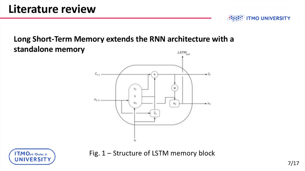
Long Short-Term Memory extends the RNN architecture with astandalone memory
Fig. 1 – Structure of LSTM memory block
7/17
8. Literature review
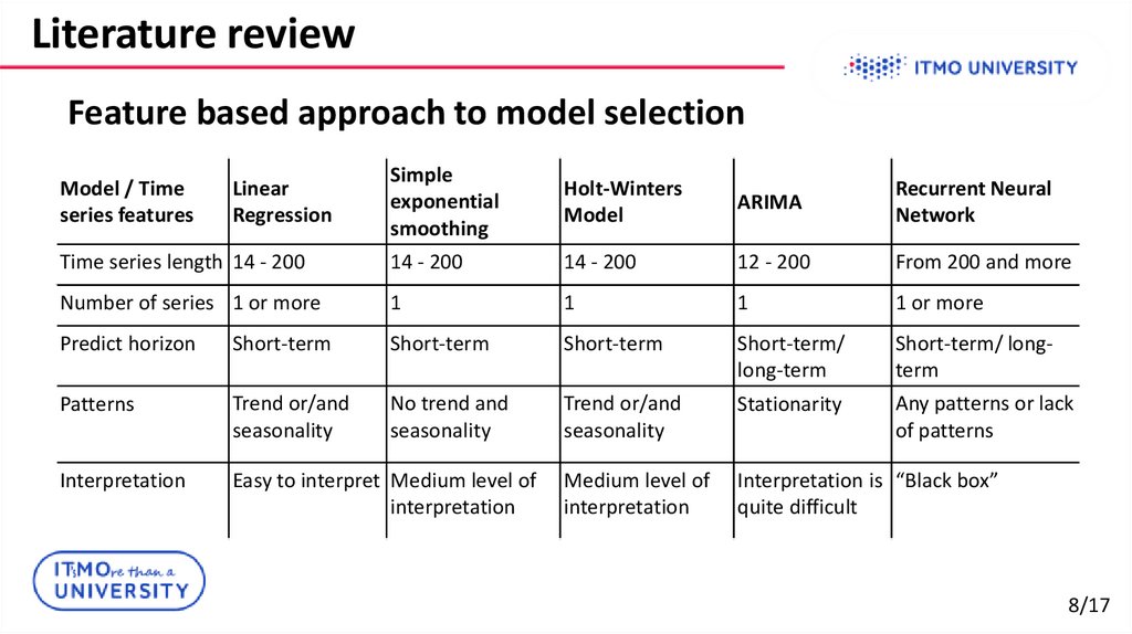
Feature based approach to model selectionSimple
exponential
smoothing
Holt-Winters
Model
ARIMA
Recurrent Neural
Network
Time series length 14 - 200
14 - 200
14 - 200
12 - 200
From 200 and more
Number of series 1 or more
1
1
1
1 or more
Predict horizon
Short-term
Short-term
Short-term
Short-term/
long-term
Short-term/ longterm
Patterns
Trend or/and
seasonality
No trend and
seasonality
Trend or/and
seasonality
Stationarity
Any patterns or lack
of patterns
Interpretation
Easy to interpret Medium level of
interpretation
Medium level of
interpretation
Interpretation is “Black box”
quite difficult
Model / Time
series features
Linear
Regression
8/17
9. Literature review
Algorithm of modelselection
9/17
10. Model comparison
Training details:Linear Regression
- 91 parameters including bias
Holt-Winters Model
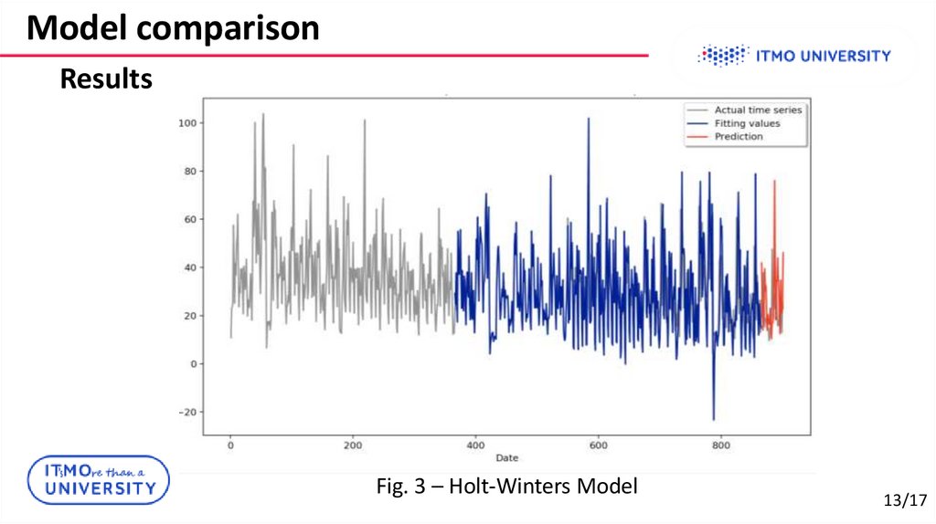
- alpha = 0.55, beta = 0.01, gamma = 0.85
Recurrent Neural Network
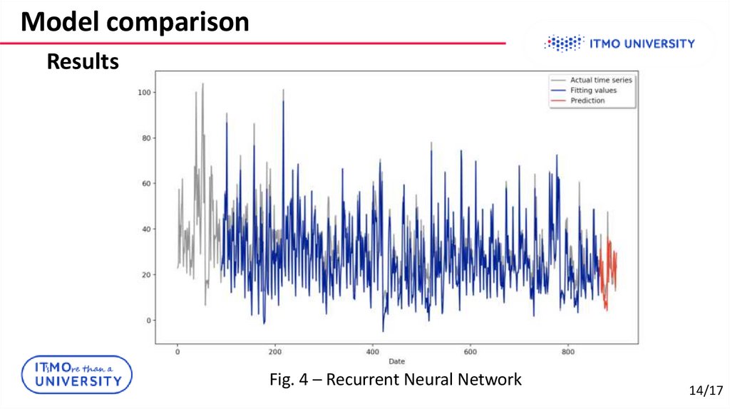
- LSTM with 1 layer, with 512 cells.
- The input shape was defined as 1 time series step with 90 features.
- Stochastic gradient descent with fixed learning rate of 0.01 was used as
optimizer, loss-function – Mean Squared Error.
10/17
11. Model comparison
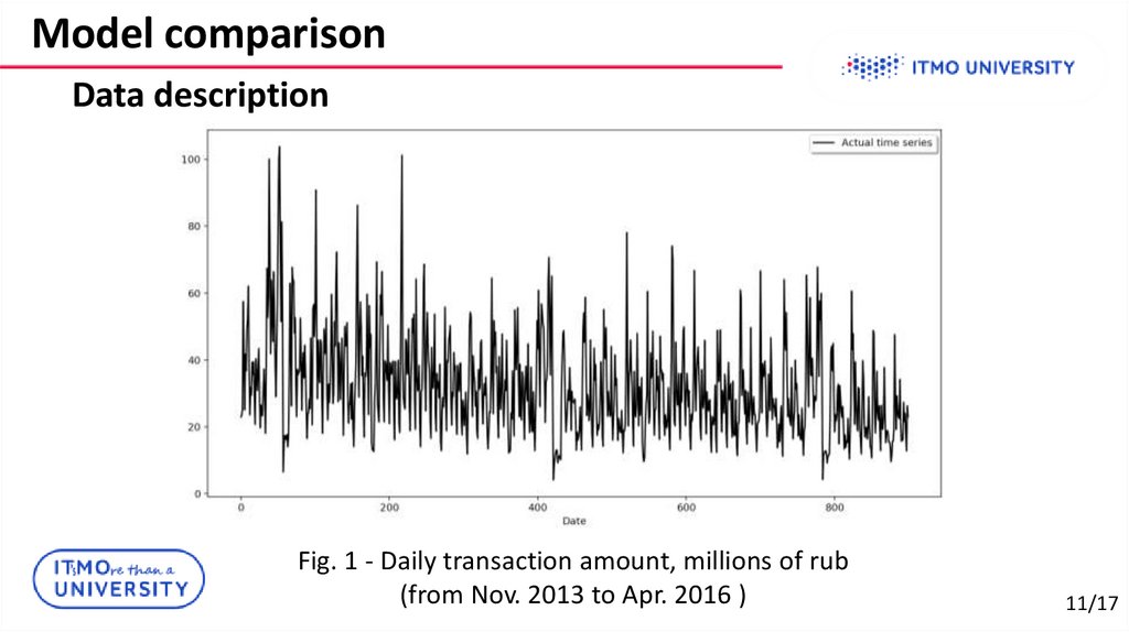
Data descriptionFig. 1 - Daily transaction amount, millions of rub
(from Nov. 2013 to Apr. 2016 )
11/17
12. Model comparison
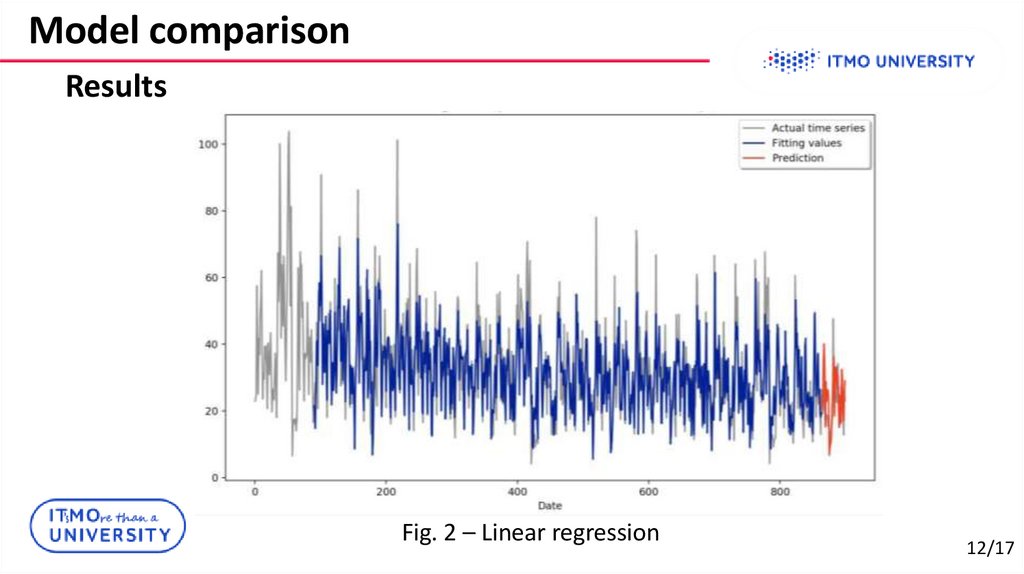
ResultsFig. 2 – Linear regression
12/17
13. Model comparison
ResultsFig. 3 – Holt-Winters Model
13/17
14. Model comparison
ResultsFig. 4 – Recurrent Neural Network
14/17
15. Model comparison
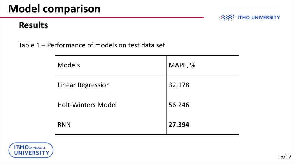
ResultsTable 1 – Performance of models on test data set
Models
MAPE, %
Linear Regression
32.178
Holt-Winters Model
56.246
RNN
27.394
15/17
16. Outputs
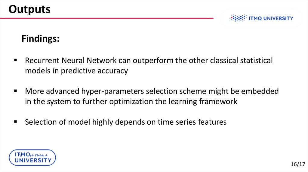
Findings:Recurrent Neural Network can outperform the other classical statistical
models in predictive accuracy
More advanced hyper-parameters selection scheme might be embedded
in the system to further optimization the learning framework
Selection of model highly depends on time series features
16/17
17. Further work plan
Plan:Optimization Recurrent Neural Network parameters to achieve more
accurate result:
Review and apply different configuration of RNN
Review and apply different attention mechanism
Generate new features
Select model with the best configuration and valuate model attention
Compare with baseline LSTM-model
17/17




 english


