


 english
Similar presentations:


Classification of Body Postures and Movements Data Set
1.
Classification of Body Posturesand Movements Data Set
CSCI 4364/6364
Fall 2015
Liwei Gao, Yao Xiao
2.
Purpose of Project• With the rise of life expectancy and aging of population, the
development of new technologies that may enable a more
independent and safer life to the elderly and the chronically ill has
become a challenge.
• The purpose of the project is to build a model, which uses the data
from wearing sensors to predict the body postures and movements of
the elder or ill. This would reduce the treatment costs.
3.
Dataset• Wearable Computing: Classification of Body Postures and Movements
(PUC-Rio) Data Set. (UCI Machine Learning Repository)
• The dataset includes 165,632 instances with 18 attributes.
• It collects 5 classes (sitting-down, standing-up, standing, walking, and
sitting) on 8 hours of activities of 4 healthy subjects.
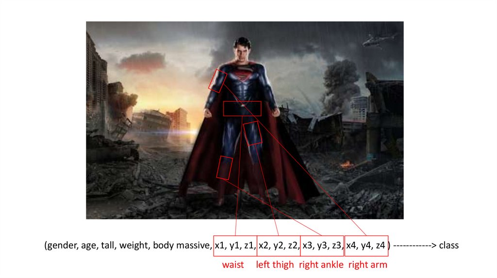
• The dataset may be divided into two parts: the information of the
subjects (gender, age, tall, weight, body massive index) and data from
4 accelerometers.
4.
(gender, age, tall, weight, body massive, x1, y1, z1, x2, y2, z2, x3, y3, z3, x4, y4, z4 ) ------------> classwaist
left thigh right ankle right arm
5.
Models of Project• SVM with Linear Kernel
• SVM with Polynomial Kernel
• SVM with RBF Kernel
• Decision Tree
• Random Forest
• Gradient Boosting (GBDT)
• Neural Networks
6.
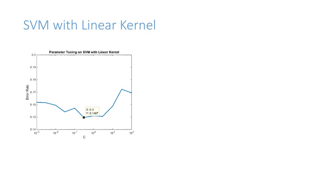
SVM with Linear Kernel7.
SVM with Polynomial Kernel8.
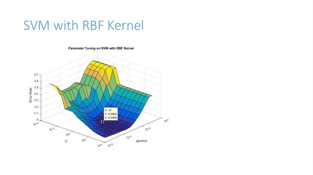
SVM with RBF Kernel9.
Decision Tree10.
Random Forest11.
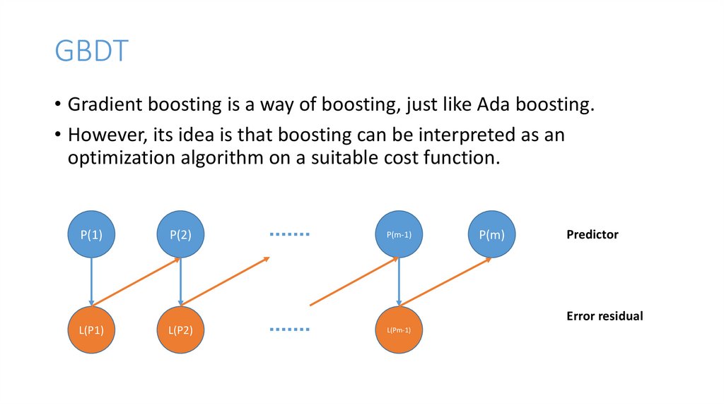
GBDT• Gradient boosting is a way of boosting, just like Ada boosting.
• However, its idea is that boosting can be interpreted as an
optimization algorithm on a suitable cost function.
P(1)
P(2)
P(m-1)
P(m)
Predictor
Error residual
L(P1)
L(P2)
L(Pm-1)
12.
GBDT• Review what we learned in Ada boosting. In Ada boosting, we change the weight of
points after each training, then we train again.
• In gradient boosting, we compute the loss function(error residual) of each weak learner,
which is a function of parameter set P, then do gradient descent for this function and get
a better learner. We add these two learner and get new complex learner P2.
P(1)
P(2)
P(m-1)
P(m)
Predictor
Error residual
L(P1)
L(P2)
L(Pm-1)
13.
GBDT• There are some important parameters when we use GBDT.
• n_estimators: The number of boosting stages to perform. Gradient
boosting is fairly robust to over-fitting so a large number usually
results in better performance.
• learning_rate: It shrinks the contribution of each tree, the bigger the
faster (overfit). It is a trade-off with n_estimators.
• max_depth: maximum depth of each decision trees. Deep trees are
easy to result in overfitting.
14.
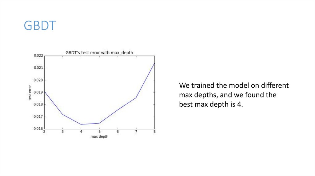
GBDTWe trained the model on different
max depths, and we found the
best max depth is 4.
15.
GBDTTo reduce the time complexity, we
also trained the model on different
size of train data. And we found
the size is over 4500, it doesn’t
improve the accuracy much.
16.
Neural NetworkInput Layer: 17 features as 17 inputs;
Output Layer: 5 outputs. (Then take the index of highest output as class);
Hidden Layer: After several tests, we used three hidden layers (13,11,7).
Connections: feed forward net.
Some Advice for Hidden Layer:
• The optimal size of a hidden layer is usually between the size of the input and size of
the output layers.
• More layers instead of more neurons on each layer.
• 1 or 2 hidden layers or use mean of input and output as neuron number can get a
decent performance.
17.
Neural NetworkHidden Layer Accuracy(%)
11
14
(10 9)
(13 9)
(13 9 7)
(14 11 8)
(13 11 7)
Our NN model has little improvement
after 24 epoch in training.
93.76
93.71
95.37
96.06
95.86
95.93
96.35
Some representative hidden layer test
shows as table.
18.
Ensemble of Models• We combined 7 models
into a ensemble model.
• The weight of each model
1
is 2 , where